XMLLR for Improved Speaker Adaptation in Speech Recognition Daniel Povey, Hong-Kwang J. Kuo IBM T.J. Watson Research Center, Yorktown Heights, NY, USA {dpovey,hkuo}@us.ibm.com

Abstract In this paper we describe a novel technique for adaptation of Gaussian means. The technique is related to Maximum Likelihood Linear Regression (MLLR), but we regress not on the mean itself but on a vector associated with each mean. These associated vectors are initialized by an ingenious technique based on eigen decomposition. As the only form of adaptation this technique outperforms MLLR, even with multiple regression classes and Speaker Adaptive Training (SAT). However, when combined with Constrained MLLR (CMLLR) and Vocal Tract Length Normalization (VTLN) the improvements disappear. The combination of two forms of SAT (CMLLR-SAT and MLLR-SAT) which we performed as a baseline is itself a useful result; we describe it more fully in a companion paper. XMLLR is an interesting approach which we hope may have utility in other contexts, for example in speaker identification. Index Terms: speech recognition, speaker adaptation, MLLR

1. Introduction In the popular speaker adaptation technique called Maximum Likelihood Linear Regression (MLLR) [1], the means are adapted per speaker using an affine transform: (s)

µ ˆj = A(s) µj + b(s) . (1) This is often combined with the use of regression classes [2], in which the transform parameters A(s) and b(s) depend on the particular Gaussian j; sometimes there are just two regression classes corresponding to silence and non-silence, sometimes a variable number based on a tree of clustered phones. The technique we are proposing here we are calling eXtended MLLR (XMLLR); it is a mean adaptation technique where we do, per speaker: (s)

µ ˆj

(s)

= µj + A(s) nj ,

(2)

(s)

where A is a speaker-specific transformation and nj are vectors which we associate with each Gaussian j. We compute these associated vectors nj using an ingenious eigenvalue based method; this invites comparison with Eigenvoices [5] but our technique has a much higher ratio of speaker-specific parameters to global parameters. This technique is also similar to the Cluster Adaptive Training approach B-CAT [4], but the initialization technique and other details differ. Section 2 describes the method by which we initialize the associated vectors; Section 3 describes how we further optimize them; Sections 4 and 5 gives experimental conditions and results, and Section 6 concludes.

2. Eigen decomposition method of initializing associated vectors In this section we describe an eigenvalue based method of initializing the vectors nj . The method assumes we have a system

already trained (i.e. the means and variances, but not the associated vectors), and it must have a number of Gaussians J less than about 10,000 so it we can fit in memory a matrix of that dimension. We can use this initialization to bootstrap a larger system. Suppose the associated vectors nj are of size E (say, E = 80) and we have a total of, say J = 5000 Gaussians 1 ≤ j ≤ J in our HMM set. Let N be a tall (J × E) matrix, the j’th row of which is nj . We can write the overall improvement in the auxiliary function that we obtain from our adaptation technique, as a function of N, as follows. Firstly, let us compute the improvement in likelihood from speaker s and feature dimension 1 ≤ d ≤ D where D is the total feature dimension e.g. 40. In the follow(s) ing we use the fact that Nad is a column vector representing the change in the mean of Gaussians 1 through J for dimen(s) sion d of speaker s; ad is the d’th row of speaker transform (s) A . It is helpful to think of each pair (s, d) as like a separate single-dimensional “sub-speaker.” Our auxiliary function improvement for “sub-speaker” (s, d) is: (s) T

f (s, d) = vd

(s) T

(s)

Nad − 0.5ad

(s)

(s)

NT diag(wd )Nad , (3)

where diag(·) means making a matrix whose diagonal is the given vector, and we define (s) PT xd (t)−µj,d (s) (s) vd,j = (4) t=1 γj (t) σ2 j,d

(s) wd,j (s)

=

(s) 1 t=1 γj (t) σ 2

PT

.

(5)

j,d

(s)

vd,j and wd,j represent the linear and quadratic terms in the objective function for the mean-offset of Gaussian j, speaker s (s) and dimension d. We write γj (t) and x(s) (t) for the Gaussian (s)

posteriors and features. We can solve (3) for ad : “ ”−1 (s) (s) (s) ad = NT diag(wd )N NT vd ,

(6)

and substituting this into Equation 3 and simplifying we get: “ ”−1 (s) (s) T (s) NT vd . (7) f (s, d) = 0.5vd N NT diag(wd )N The overall objective function is a sum over all f (s, d). This is starting to look like an eigenvalue problem but we first need to (s) get rid of the diagonal matrix diag(wd ) in the middle. We will do this as best we can by using appropriate per-speaker, perGaussian and per-dimension constants to make the remaining elements as close to unity as possible, and then ignore them. (s)

2.1. Approximating wd (s)

In approximating wd we use the following things: we compute the average per-dimension variance σ ¯d2 over all the Gaussians in our model; we also use the number of frames Ts for

each speaker, and the prior pj of Gaussian j (these sum to one over all Gaussians); we also compute a constant cj = PD σ¯ d2 1 which is large if Gaussian j has smaller than avd=1 σ 2 D j,d

(s)

1 2 Ts pj cj . σ ¯d (s) constant kd

erage variances; we can then approximate wd,j ≃ (s)

We break down wd into a “sub-speaker”-specific ¯ where multiplied by an “average” value w, (s)

3.1. Computing per-speaker matrices A(s) The computation of per-speaker adaptation matrices A(s) is similar to the MLLR computation [1]. We first adapt the means using any previous speaker adaptation matrix used and any current associated vectors, and compute the Gaussian posteriors. Then we compute per-speaker statistics as for ML training but (s) omitting the variance, i.e. we accumulate counts γj , and data

≃

(s) ¯ kd w

(8)

sums xj

(s) kd

=

Ts /¯ σd2

(9)

¯j w

=

1 pj D

dimension d a vector vd and matrix Md that appear in our objective function:

wd

2 σ ¯d d=1 σ 2 j,d

PD

We can then approximate the objective function as: ` ´−1 T (s) P (s) T ¯ f ≃ s,d 0.5 N NT diag(w)N N vd . (s) vd kd

(10)

(s)

From these statistics we accumulate for each feature (s)

f (s, d) (11)

2.2. Eigenvalue solution for N We can then solve for N by using the substitution ¯ 0.5 N O = diag(w) (12) The objective function then becomes: “ ” X 0.5 (s) T −0.5 T ¯ ¯ −0.5 vd(s) . v diag( w) O O O OT diag(w) f≃ d (s) s,d kd (13) We can make the arbitrary stipulation that OT O = I (we can show that it does not matter what this is as long as it is nonsingular). Then we can see that the columns of O are the principal eigenvectors of M, where S X D X T 0.5 ¯ −0.5 vd(s) vd(s) diag(w) ¯ −0.5 . M= diag(w) (s) s=1 d=1 kd (14) ¯ −0.5 O. We can then set N = diag(w) 2.3. Computation for initialization of XMLLR For a small system (we use 5000 Gaussians for the initialization) we can compute the matrix M quite efficiently. For each speaker we accumulate statistics as for ML training (count and (s) mean; variance is not needed); from this we can get vd for this speaker and each dimension and accumulate its weighted outer P(s) (s) (s) (s) T product; that is, accumulate the sum . d 1/kd vd vd (s) We take into account the sparseness of vd when accumulating the outer product and iterate over a list of nonzero indexes. We do this in parallel for different blocks of data, sum up the ¯ −0.5 prior to finding the top different parts and then scale by w eigenvectors. Doing a singular value decomposition (SVD) on M for dimension 5000 should take about 1 hour at 1GFLOP assuming SVD takes O(30n3 ) operations; in fact we use a very fast method which we will not describe here.

(s)

(s) T

(s)

=

C + ad

(s)

=

Ts X J X

(s)

=

(s) Ts X J X γj (t) nj nTj 2 σ j,d t=1 j=1

vd

Md

(s) T

vd − 0.5ad

(s) x (t) − (s) γj (t) d 2 σj,d t=1 j=1

(s)

(s)

(s) (s)

(15)

nj

(16)

M d ad

µj,d

(17)

(s) −1

We then solve ad = vd Md . We also enforce a perdimension of cmin frames; by default we use 10 for this. Thus, (s) (s) if necessary we truncate the dimension of vd and Md to (s) T /cmin and use zero for any remaining dimensions in ad . This makes sense because the dimensions of nj are sorted by eigenvalue. 3.2. Re-computing associated vectors nj 3.2.1. Full computation The most exact (but expensive) form of the computation of the associated vectors nj is similar in requirements to Speaker Adaptive Training [6] but in the dimension E which in our case is 80. Like the computation above it requires computing vectors vj and matrices Mj which form an auxiliary function f (j) as follows: =

vjT nj − 0.5nTj Mj nj

vj

=

Ts XX

Mj

=

(s) Ts XX γj (t) (s) (s) T ad ad . 2 σj,d s,d t=1

f (j)

(s) x (t) − (s) γj (t) d 2 σj,d s,d t=1

(18) µj,d

(s)

ad

(19)

(20)

The solution is then nj = vj M−1 j . As for the per-speaker ma(s)

trices, the Gaussian posteriors γj (t) must be obtained using the current adapted form of the Gaussians. 3.2.2. Quick computation

3. Iterative optimization in XMLLR After initialization of the associated vectors nj we start an iterative process where we first compute the per-speaker matrices A(s) , then recompute the per-Gaussian associated vectors nj , and then re-estimate the Gaussian mixture weights and parameters µj and Σ2j ; we do each of these three steps for 4 iterations in experiments reported here. If we want to convert to a larger size system, at that point we use the per-speaker matrices A(s) to compute the associated vectors nj for the larger system and start 4 iterations of the same process on the larger system. This requires that the smaller and larger system share the same features.

We also used a quick form of the computation of the associated vectors nj , which we found to be as effective as the full form. This relies on storing only the diagonal of the quadratic term Mj for most Gaussians j, but storing the full Mj for a subset K of Gaussians (we use 1 in E of the total). We then do a diagonal update of nj , but using dimension specific learning rate factors l = le , 1 ≤ e ≤ E which are learned from the subset for which we stored the full matrix. These should be between zero and 1 (in fact we enforce 0.1 ≤ le ≤ 1). We formulate the computation as an update to nj . The computation (s) becomes (note the dependence now on the adapted mean µ ˆj ):

vj

=

Ts D X S X X

(s)

(s)

γj (t)

s=1 d=1 t=1

Mj

=

(s) Ts D X S X X γj (t)

=

X

vj,e

X

Mj e,f

s=1 d=1 t=1

we

j∈K

Ne,f =

j∈K

l nj,e

= :=

2 σj,d

(s)

xd (t) − µ ˆj (d) (s) ad 2 σj,d (s) (s) T

ad ad

vj,e Mj e,e vj,e vj,f Mj e,e Mj f,f

wN−1 vj,e nj,e + le Mj e,e

XMLLR or in MLLR decoding without SAT). In both the SI and SA cases we show experiments on a small model with 700 quinphone context-dependent states and 5k Gaussian mixture components, and a larger system with 1000 states and 30k Gaussians (SI) or 3000 states and 50k Gaussians (SA). As a baseline for XMLLR because it includes SAT-like elements we compare against (MLLR-)SAT, which we implement as ML-like SAT as described in a companion paper [7]. The language model is a small (3.3M n-grams) interpolated back-off 4-gram model smoothed using modified Kneser-Ney smoothing. It was trained on a collection of 335M words from various public data sources, mostly released by LDC. The vocabulary size is 84K words. The test set consists of the dev04 English Broadcast News development set, a total of 2.06 hours.

3.2.3. Gaussian update We also update the Gaussian parameters using a form of Speaker Adaptive Training which is appropriate for our technique. Essentially the update consists of viewing the speaker adaptive modification to our Gaussian mean, as a modification of the opposite sign to our features. Writing the speaker(s) (s) specific counts and mean and variance statistics as γj , xj (s)

and Sj , and if the speaker adaptive update to the mean is (s) mj

(s)

=µ ˆj − µj = A(s) nj , then PS (s) γj = (21) s=1 γj PS (s) (s) (s) (22) xj = s=1 xj − γj mj PS (s) (s) (s) (s) (s) T Sj = . (23) s=1 Sj − 2xj mj + mj mj

Since we have diagonal Gaussians we only store the diagonal of the variance statistics Sj . This approach requires storing two sets of Gaussian statistics in memory, one used to make speaker statistics and one used to store total statistics.

4. Experimental Setup Our experiments use an English broadcast news transcription system. The acoustic models are trained on 50 hours of audio obtained by sampling entire shows from the 1996 and 1997 English Broadcast News Speech corpora. The recognition features are 40-d vectors computed via an LDA+MLLT projection of 9 spliced frames of 13-d PLP features. Features for the speakerindependent (SI) system are mean-normalized, while features for the speaker-adapted (SA) system are mean- and variancenormalized. In both cases, normalization statistics are accumulated per speaker. The LDA+MLLT transform is computed by interleaving semi-tied covariance estimation using a single, global class and HMM parameter estimation during system training to diagonalize the initial LDA projection. In the training of the speaker-adapted system we use both vocal tract length normalization (VTLN) and Constrained MLLR (CMLLR). The acoustic models are trained using maximum likelihood estimation. There are either two or four decoding passes, each using adaptation based on the transcripts from the previous stage. In the SI systems we have a speaker-independent (SI) pass (cepstral mean subtraction only), and then a pass including MLLR or XMLLR. In the SA systems we have a SI pass, use this output compute VTLN warp factors for the VTLN pass, then a VTLN+CMLLR pass, then VTLN+CMLLR+(MLLR or XMLLR). In general all four passes use different HMMs (the exception is the last two, which are the same on iteration zero of

5. Experimental Results Iteration (None) 0 1 2 3 4 (all)

XMLLR 41.1% 37.9% 36.8% 36.8% 36.4% 36.3%

WER MLLR MLLR+rtree 41.1% 41.1% 38.6% 38.4% 37.1% 37.0% 37.1% 37.2% 36.6%

Table 1: Speaker Independent, small (5k Gaussian) Iteration (None) 0 1 2 3 4 (all)

XMLLR 34.1% n/a 30.5% 30.1% 29.8% 29.7%

WER MLLR MLLR+rtree 34.1% 34.4% 31.7% 31.9% 30.9% 30.9% 30.9% 30.7% 30.2%

Table 2: Speaker Independent, normal (30k Gaussian) Iteration (None) 0 1 2 3 4

XMLLR 33.9% 33.3% 33.1% 33.0% 32.9% 32.7%

WER MLLR+rtree 33.9% 33.2% 33.1% 33.0% 32.8% 32.8%

Table 3: Speaker Adapted, small (5k Gaussian) In these experiments, we show results without MLLR or XMLLR in rows marked “(None)”, and with XMLLR and MLLR on various iterations of training. XMLLR iteration zero is after initialization of the associated vectors; following iteration numbers are iterations of updating everything (transforms, associated vectors using the quick approach, Gaussian parameters). MLLR iteration zero is a system without (MLLR-)SAT, and following iterations are iterations of SAT; iteration “(all)” means doing a system build from scratch with SAT; details on SAT training are in [7].

Iteration (None) 0 1 2 3 4 (all)

XMLLR 26.0% n/a 25.0% 25.0% 25.0% 25.0%

WER MLLR+rtree 26.0% 25.3% 25.2% 25.2% 25.1% 25.1% 24.9%

Table 4: Speaker Adapted, normal (50k Gaussian) Iteration Full 41.1% 37.9% 36.7% 36.7% 36.5% 36.3%

(None) 0 1 2 3 4

WER (XMLLR) Quick ...and no SAT 41.1% 41.1% 37.9% 37.9% 36.8% 37.7% 36.8% 37.6% 36.4% 37.7% 36.3% 37.5%

Table 5: Building style: (SI, small: 5k Gaussian) Tables 1 and 2 show our technique on small and larger size speaker independent models. Comparing against MLLR without SAT, the improvements are quite impressive: 1.9% and 2.2% absolute for the small and large system (iteration 4). However our gains are reduced if we compare against systems with SAT: 0.3% and 0.5% respectively if we compare against systems trained from scratch with SAT. On the SA system (Tables 3 and 4), even more of our gains disappear: we get 0.5% and 0.3% respectively versus MLLR with no SAT, and 0.1% and -0.1% versus the best available SAT numbers. Table 5 compares different methods of system building for XMLLR. We see that the quick update for the associated vectors gives about the same results as the full update, and that if we omit the SAT element (i.e. the fact that we train the Gaussian parameters jointly with the adaptation parameters) we lose 1.2% absolute. We tried modifying from 10 the per-dimension minimum count used in test time; there were small improvements (0.1% to 0.2%) from changing this to the 100 to 200 range, but these may not be significant. We tried combining, in test-time, the learned associated vectors with other predictors. In one experiment we simply appended the mean to the learned associated vectors but this gave a 0.3% degradation. The improvements from XMLLR are associated with an increase in test-time likelihood. On the small SI system (Table 1) on iteration zero (just initialized) we reduced the dimension E from 80 to 40; this degraded WER from 37.9% to 38.3% which −4

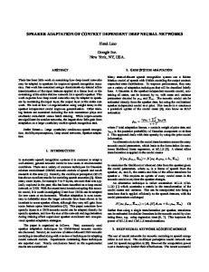
x 10

Eigenvalues Like improvement per dim 2

1

0

0

10

20

30 40 50 SPEAKER INDEPENDENT

60

70

80

−5

6

x 10

Eigenvalues Like improvement per dim

5 4 3 2 1 0

0

10

20

30

40 50 SPEAKER ADAPTED

60

70

80

Figure 1: Eigenvalues of M and likelihood improvement

it still better than non regression tree MLLR with about the same number of per-speaker parameters (at 38.6%). The unadapted test likelihood was -54.78 per frame; non regression tree MLLR adapted was -52.82, and XMLLR adapted (E=40) was -52.59. For comparison the best XMLLR result in Table 1 had likelihood of -51.19 and the best regression-tree MLLR SAT result had -51.28. All these likelihood results track WER. Figure 1 shows the eigenvalues of the matrix M, and also the objective function improvement we get from adaptation, using each dimension of the computed associated vectors separately; the improvement is computed using the initially estimated associated vectors, and scaled arbitrarily for display. Any differences are due to approximations we made in the eigenvalue initialization. The correspondence seems quite close for the SI system; however, it breaks down for the SA system. We found a correspondence between lower-than-expected objective function improvement and uneven distribution of associated vectors, meaning that for the problematic dimensions most of the Gaussians had very small associated vector values in that dimension and just a few had large values. This appears to be due to certain Gaussians having very unevenly distributed counts among speakers, which breaks our assumptions. We were able to correct this discrepancy by iteratively identifying Gaussians with larger than average factor vectors nj and decreasing their weight w ¯j−0.5 by a factor weakly dependent on the excess. This improved the objective function and WER on the first few iterations, but they both appeared to converge to the same point regardless of the initialization used (results not shown).

6. Conclusions We have introduced a form of adaptation called eXtended MLLR (XMLLR), which is a modified form of MLLR in which we regress on vectors associated with each mean. XMLLR appears to be a more powerful form of adaptation than MLLR, giving large improvements against an MLLR baseline; however, when we implemented Speaker Adaptive Training (SAT) for use with MLLR and combined these techniques with other forms of adaptation the improvements versus MLLR disappeared. Nevertheless we hope that XMLLR may prove to be useful, perhaps in a different configuration or for use in speaker identification.

7. Acknowledgements This work was funded by DARPA contract HR0011-06-2-0001.

8. References [1] Leggetter, C. J. and Woodland, P. C., “Maximum Likelihood Linear Regression for Speaker Adaptation of Continuous Density Hidden Markov Models,” Computer Speech and Language, v. 9, pp. 171-185, 1995. [2] Gales M.J.F., “The generation and use of regression class trees for MLLR adaptation,” Technical Report CUED/F-INFENG/TR263, Cambridge University, 1996. [3] Gales, M. J. F., “Maximum Likelihood Linear Transformations for HMM-based Speech Recognition,” Computer Speech and Language, v. 12, 1998. [4] Gales, M. J. F, “Multiple-cluster adaptive training schemes,” Proc. ICASSP, 2001. [5] Kuhn R., Junqua J.-C., Nguyen, P., Niedzielski, N., “Rapid Speaker Adaptation in Eigenvoice Space,” IEEE Transactions on Speech and Audio Processing, v. 8, no. 6, Nov. 2000. [6] Anastasakos, T., McDonough, J., Schwartz R. and Makhoul, J., “A Compact Model for Speaker-Adaptive Training,” Proc. ICSLP, 1996. [7] Povey, D., Kuo, H-K. J. and Soltau H., “Fast Speaker Adaptive Training for Speech Recognition,” submitted to: Interspeech, 2008.