Why did wage inequality decrease in Mexico after NAFTA? Raymundo M. Campos-Vazquez

University of California, Berkeley Department of Economics October 2008

Abstract Contrary to what happened before NAFTA, wage inequality in Mexico decreased after 1994. This paper investigates the forces behind the post-NAFTA decrease in wage inequality. Using a quantile decomposition, I show that the decline in wage inequality is driven by a decline in the returns to education and potential experience, especially at the top of the wage distribution. Supply and demand are the main contributors for this change. On the supply side, there were substantial increases in college enrollment rates after 1994, which translated into an increase in the proportion of workers with a college degree. However, this increase in supply was not met by an increase in demand for the highly educated: the proportion of the workforce in top quali…ed occupations and close to the top occupations did not increase as much as the increase in supply. As a result, college educated workers put wage pressures in top and less than top quali…ed occupations. A Bound and Johnson (1992) decomposition con…rms that changes in relative supply are the main determinant behind the decrease in wage inequality. E-mail: [email protected]. 508-1 Evans Hall #3880, Berkeley CA 94709. UC Mexus provided funding for this research. I appreciate their support. I also appreciate comments by Eva Arceo-Gómez, Daniel Egel and Kevin Stange. I am grateful to my advisors David Card and Emmanuel Saez. All remaning errors are my own.

1

1

Introduction

Inequality, either measured by income or wages, is an important topic that has been continuously debated among academics and the media. Since the 1980s, most countries in the world experienced an increase in wage inequality and for some countries this trend continued during the 1990s. Mexico was no exception and went trough a period of increasing inequality by the end of the 1980s. However, wage inequality in Mexico started to decline after 1994, the period after NAFTA was enacted. This could be surprising given the relatively large literature explaining the causes of the increase in inequality at the end of the 1980s and beginning of the 1990s.1 Figure 1 documents the patterns of wage inequality in Mexico. Even though the decline has been taking place since 1994-1996, there are basically no references for this episode in the literature.2 In this paper I try to …ll this gap and I give an explanation for the potential causes of this episode. Wage inequality has continuously increased during the last 20 years in the United States and other developed countries.3 There is a debate about the causes of this increase. On one hand, David Autor, Lawrence Katz and Daron Acemoglu among others4 argue that skill biased technical change is the leading explanation for the increase in wage inequality. Since the supply of college educated increased during the period, the only possible explanation is that demand increased by more than the supply and that the growth in demand is biased towards skilled workers. On the other hand, Thomas Lemieux, David Card and John Dinardo among others5 criticize the view of skill biased technical change as the main source for changes in wage inequality. Instead, they argue that the increase in wage inequality at the end of the 1980s and beginning of 1990s can be seen as episodic rather than driven by skill biased technical change. According to their estimates, most of the increase in wage inequality, especially at the bottom of the wage distribution, in that period can be explained by the fall in the real minimum wage and a decline in unionization rates. More recently, Autor et al. (2008) recognize changes in the real value of the minimum wage and the fall of unionization rates as plausible explanations for changes in lower tail inequality. However, they point 1

For example see the papers by Airola and Juhn (2005), Cragg and Epelbaum (1996), Esquivel and Rodríguez-López (2003), Fairris (2003), Feliciano (2001), Hanson (2003), López-Acevedo (2006), Meza (2005), Robertson (2004). 2 As explained below, I use the Expenditure Survey (ENIGH) for the analysis. The peak of wage inequality di¤ers from the one calculated using the Labor Force Survey. Wage inequality in the Labor Survey peaks in 1996, but the downward trend is very similar to the trend using the Expenditure Survey. Some recent papers like Airola and Juhn (2005) and López-Acevedo (2006) acknowledge either that wage inequality has not grown or has decreased slightly. The view in this paper is that wage inequality has decreased substantially after 1994. 3 Katz and Autor (1999), Table 10. 4 Acemoglu (2002), Autor et al. (2003), Autor et al. (2005, 2007, 2008). 5 Card and DiNardo (2002), DiNardo et al. (1996), Lemieux (2006, 2008).

2

out that institutional aspects cannot explain the continuous rise in upper tail inequality. They conclude the increase in upper tail inequality cannot be explained by quantities but by returns, justifying the view of skill biased technical change as an important source for changes in wage inequality. In some developed countries the wage structure has been changing favoring the high and low skilled workers. This process increases upper tail wage inequality but reduces lower tail inequality. For the U.S., Autor et al. (2007) show how high skilled jobs (occupations) in 1980 were the ones with the highest increase in demand, measured by the increase in the proportion of workers in those occupations. They also …nd that occupations in the lower tail increased their participation, but at the expense of middle-tier jobs. Furthermore, in the U.K., Goos and Manning (2007) …nd a similar pattern to that in the U.S. case, and call this U-shaped pattern "job polarization." They conclude that skill biased technical change and job polarization are likely explanations for the increase in wage inequality. In another study on Germany, Dustmann et al. (2007) and Spitz-Oener (2006) …nd that job polarization is present and the increase in wage inequality can be explained in part by that process. As explained above, inequality has continuously increased in developed countries since the 1980s. In contrast, Mexico exhibits a decrease in inequality after 1994, and in this paper I explore the causes of such a decline. This is important for at least three reasons. First, societies generally value a more egalitarian distribution of resources. Hence the example of Mexico may be useful to other similar countries that desire to attain lower inequality levels. Second, the analysis of Mexico is interesting because it can shed some light on the role and nature of skill biased technical change. If the use of computers is an important source for skill biased technical change, then we expect Mexico’s labor demand to behave similar to other countries given that Mexico also experienced an important decline in the price of computers.6 Finally, it is also interesting to investigate whether Mexico has "job polarized" as other countries and analyze how this process modi…es the wage distribution. In order to analyze the sources of the fall in wage inequality, I follow Mata and Machado (2005) decomposition. In particular, I estimate quantile regressions and build counterfactuals of the wage distribution holding constant observable characteristics or returns in schooling and potential labor experience. This decomposition is similar to DiNardo et al. (1996) non-parametric decomposition. The goal is to estimate the level of inequality using the endowments from one speci…c year but assuming returns values for a di¤erent year and vice versa. The results of the decomposition show that the returns to education and labor experience are the most important factor explaining the decrease in wage inequality. The 6

See for example Autor et al. (2003). They argue that the decline in the price of computers is the causal mechanism for the increase in demand of top quality jobs.

3

decline in returns is explained by a substantial increase in college graduates in the last 10 years, but it is also due to slower growth in labor demand, especially for the top paid jobs. I divide jobs by "quality" using the occupation median wage in 1992 and show that top quality jobs did not grow as much as the increase in supply of high-skilled workers. Instead, low wage jobs increased their participation substantially at the expense of above the median wage jobs. In order to present further evidence on my …ndings, I decompose the relative wage changes as in Bound and Johnson (1992). These results con…rm that changes in relative supply are the main determinant behind the decrease in wage inequality. The paper is structured as follows. In the next section I describe the basic facts and trends of wage inequality in Mexico for di¤erent groups. Then I question and contrast di¤erent hypotheses of the decline of wage inequality in the last years. The next section carries the Mata and Machado (2005) methodology to decompose wage inequality, I present results for this decomposition and then analyze whether job polarization has occurred in Mexico and relate this process to the change in wage inequality. I then calculate the percent e¤ect driven by supply and the percent e¤ect driven by demand factors following the Bound and Johnson (1992) decomposition. The last section o¤ers some concluding remarks.

2

Facts

There are three sources of data in Mexico that can be used to calculate wage inequality: Expenditure Survey, Labor Survey and the Census. Census data is not used given that there are only two points in time (1990 and 2000) and most of the decline in wage inequality is for the period 1998-2006. The labor survey has two drawbacks: it is not nationally representative given that it only has data for urban areas, and, more importantly, its methodology changed after 2004 rendering it useless for my purposes. For those reasons, my analysis will be based on the Expenditure survey (ENIGH, for its Spanish acronym). The ENIGH is nationally representative and it includes relevant variables such as income sources, expenditures and demographic characteristics. Despite the fact that the survey’s sample size is small and it is only available for years 1989, 1992 and every two years after this date including 2005, I decided to use this survey given the homogeneity of methodology during the whole period.7 In what follows I restrict the sample to all workers 18-65 year old with positive hours 7

Wage income and the de…nition of occupations are comparable throughout the period. These are two key variables in my analysis. The Labor Survey (ENEU) can be compared for urban areas from 1989 until 2003-2004 depending on the number of cities included in the analysis. As wage inequality still decreased for the period 2003-2006, I use the Expenditure survey to take into account this latter period. It is important to clarify that the pattern of wage inequality in the Expenditure Survey is similar to the pattern in the Labor Survey, the di¤erence that the peak in wage inequality is in 1996 instead of 1994.

4

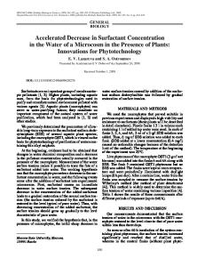
of work and valid wage. When calculating hourly wage I follow Airola and Juhn (2005) and calculate monthly wage over 4.33 times hours of work, and when calculating descriptive statistics I use as a weight the person weight from the data times hours of work as is commonly used in the wage inequality literature. Wages are in constant 2006 Mexican Pesos. I drop observations with real hourly wage less than $1 MXP.8 I do not restrict the sample to fulltime workers, but in the Appendix I show some of the results presented below including just full-time workers as well as using other de…nitions of income.9 Figure 1 plots the trends of wage inequality in Mexico since 1989 using the log di¤erence between the 90th and 10th percentile. As has been documented in the literature, Mexico experienced a large increase in wage inequality in the period before 1994. What has not been documented as widely is the substantial decrease in wage inequality after 1994. This decline in wage inequality applies to both males and females, although the decline is more consistent for males. Wage inequality has decreased by more than 20 log points during this period. Figure 2 and Figure 3 decompose wage inequality using the log di¤erence between the 90th and 50th and the 50th and 10th percentile respectively. Figure 2 shows a decline in top wage inequality while Figure 3 shows a decline in bottom wage inequality but not as strong as the decline in top wage inequality. Figure 1 and Figure 2 exhibit a decline in wage inequality mainly driven by top wage inequality. In the Appendix, Table 6 presents di¤erent calculations of wage inequality using the standard deviation of log wages and the Gini coe¢ cient as well as using di¤erent de…nitions of income. As we can see in this table, inequality has gone down since 1994 independently how it is measured. For example, the Gini coe¢ cient has decreased 0.06 units and when measured by the standard deviation of log wages it has decreased by 0.04 units. These are substantial decreases considering the increase in wage inequality during 1989-1994. For example the Gini coe¢ cient increased by 0.08 and the standard deviation measure by 0.09 units. The Gini coe¢ cient and the standard deviation measure show a decline in wage inequality, but cannot distinguish the decline in wage inequality in the lower or upper part of the wage distribution. For this reason, I focus mainly in the di¤erence between percentiles 90th and 50th and 50th and 10th as measures of lower and upper tail inequality. In order to analyze more carefully the change in wage inequality during 1994-2006, Figure 4 presents the change in the log wage by centiles of the wage distribution using years 1994 8

I experimented with di¤erent trimming regions and the trends of wage inequality were not a¤ected. In order to keep as many observations as possible, I only drop observations with real hourly wage less than $1 MXP because the log transformation a¤ects these values substantially. 9 In the ENIGH, I de…ne wage income consistently across surveys as "Wages" only coming from Labor Income. This term represents most of total labor income and total income. I calculated results (not reported) using total labor income and the results were similar to those obtained in the Appendix.

5

and 2006.10 For example, the …rst decile (up to quantile 10) experienced an increase in real wages close to 5 percent between 1994 and 2006. This graph indicates that there was an increase in the real wage for workers at the bottom half of the wage distribution. In fact, percentiles in the top half experienced a decrease in real wages and this decline was even larger for top percentiles (although again for women this is not the case). The real wage of the top decile decreased on average 30 percent. The Mexican Peso crisis at the end of 1994 cannot explain the full decline in wage inequality during this period.11 For example, Figure 5 exhibits a similar plot to Figure 4 but using years 1996 and 2006 instead of 1994 and 2006. Real wages at the top are still declining in comparison to di¤erent wages across the wage distribution, especially those at the very top. Deciles 2-4 had the highest wage increases during the whole period. Finally, Figure 6 plots the change in wage inequality for years 1989-2006. Wages for the bottom half of the distribution (males and females) were more or less constant, with substantial increases for the very poor. The real losers in this period were the "middle-class" and some high earners. Wages for workers between the 50th and 80th percentile decreased by close to 5 percent on average. Wages for workers between the 80th and 90th percentile decreased by close to 3 percent on average. The top decile increased their wages by close to 6 percent on average. On the other hand, females substantially improved their wages at the top of the distribution. The message in …gures (4)-(6) is that the evolution of wage inequality in Mexico needs to be separated before and after NAFTA. In sum, Figure 1 demonstrates that something a¤ected the Mexican economy during the period 1994-2006 causing a decline in wage inequality. Table 1 analyzes this issue more carefully and presents information on how real wages have evolved for di¤erent groups of workers. I follow Autor et al. (2008), and analyze subgroups of workers divided by gender, education (less than Secondary, Secondary, High School and College), and potential experience (1-20 years of experience and more than 20 years of experience) for a total of 16 groups. Then I calculate mean wages for each group and the proportion of workers in that group. In the Appendix, Table 7 includes the calculation for di¤erent measures of income, like mean hourly wage for full-time workers, monthly wage and monthly total income. Table 1 shows the decline in real hourly wage after the Mexican Peso crisis of 1994. As we can observe wages have been stagnant after 2000. This is also true for other measures of income as presented in the Appendix. The wages of workers with less than a high school 10

Given the small sample size of ENIGH, the use of centiles causes missing wages for some centiles, especially for women. For this reason, I aggregate the information every two centiles. 11 Mexico experienced a deep contraction in economic activity in 1995. GDP fell by 7 percent in 1995 and in‡ation increased by 50 percent in 1995. As shown in …gures, nominal wages did not adjust completely to the increase in in‡ation resulting in lower real wages.

6

degree increased the most for the period after NAFTA. Looking at the education groups, it is surprising that wages of workers with a high school degree and a college degree have gone down after 2000. At the same time, we can notice there was an increase in the proportion of workers with high school and college degrees during the period 1989-2006, especially for women. Table 1 presents evidence that there is a striking di¤erence in terms of the proportion of workers with di¤erent educational levels. While workers with secondary education increased their proportion in the workforce by 6 percentage points between 1989 and 1996, their proportion only increased 1 percentage point between 1996 and 2006. In contrast, workers with high school increased only 2 percentage points their participation between 1989 and 1996 while college workers increased their participation only by 1 percentage point, but for the period 1996-2006 the proportion increased by 6 and 5 percentage points between 1996-2006, respectively.

3

Hypothesis

The main hypothesis in the paper is that changes in the wage structure in Mexico for the post-NAFTA period are driven primarily by supply and demand forces. Institutional factors like unionization rates and the real minimum wage have been constant throughout the period and, as a consequence, they are unable to explain the decline in wage inequality, even more so for the decline in top wage inequality. Figure 7 depicts the trend of unionization rates and real minimum wage for the period 1989-2006. Before 1994 there is a sharp decline in both unionization rates and the minimum wage. Unionization rates fell almost 6 percentage points during 1989-2006, and the minimum wage lost 30 percent of its real value.12 However, for the period 1996-2006 both unionization rates and real minimum wage were fairly constant. The real value of the minimum wage practically did not su¤er any changes while unionization rates fell by 2 percentage points, although this fall was mainly driven for the year 2006. As institutional factors were not signi…cantly altered during the period 1996-2006, the causes of the decline in wage inequality, especially at the top, need to be found elsewhere. It is possible that a constant minimum wage helped to keep constant lower tail inequality, but it is hard to argue that a constant minimum wage caused a decline in top wage inequality. 12

There are some papers analyzing the role of unions and minimum wage on inequality in Mexico. Fairris (2003) and Fairris and Levine (2003) analyze the role of unions and Kaplan and Novaro (2006) and Bosch and Manacorda (2008) analyze the e¤ect of the minimum wage on the wage structure and wage inequality during the 1989-1994 period and later periods. In particular, Kaplan and Novaro (2006) argue that although the minimum wage is not binding in Mexico it a¤ects other wages in the distribution. Bosch and Manacorda (2008) argue that the increase in wage inequality for the period 1989-2000 can be explained by a falling real minimum wage, especially for years 1989-1996.

7

I argue that there are two main reasons for the decline in wage inequality. The …rst reason is the substantial increase in schooling after 1990, especially in the second half of the 1990s. The second reason involves an absence of top quality jobs creation. Figure 8 plots total school enrollment and Figure 9 shows enrollment rates adjusting for population since 1980.13 Before 1994 there is no substantial increase in enrollment rates. High School education increased slightly but this increase is mainly driven by the increase during 1980-1985, and after 1985 enrollment did not increase. College enrollment was fairly constant during the period 1980-1994. Supply of skilled workers did not change for the period before 1994. As enrollment rates for college and high school increased substantially after 1994, and as college usually requires 4 years of education, we expect college enrollment to have an e¤ect on wages for year 2000 and afterwards. Figure 10 plots the relative wage and relative supply of male workers with Secondary education and College education in logs levels. The …rst y-axis includes the log of the ratio of wage between secondary and college educated workers. The second y-axis includes the proportion of workers in the same education categories. Both wages and proportion of workers are obtained from the estimates provided in Table 1. The trend in proportion of workers has been smoothed using a simple moving average, I multiply the previous and post period by 0.25 respectively and add the current period times 0.50. Before 1994, the trends cannot be related with each other. After 1996 and especially after year 2000 inclusive, the trends between wages and proportion of workers are negatively correlated. The timing of the decline in relative wages coincides with the expansion of enrollment rates for college education shown in Figures 8 and 9 (adding the 4 years of college education). Assuming that other factors like demand and skill biased technical change are negligible, Figure 10 implies that the elasticity of substitution between secondary and college workers is slightly above unity.14 This elasticity implies that, holding constant other factors, a decrease 13 Enrollment data is available online through Secretaria de Educacion Publica website http://www.sep.gob.mx. Population data is obtained through the Statistical O¢ ce http://www.inegi.com.mx using Census data. I adjust for population in the following way. There are di¤erent age groups in the Census as reported by the Statitiscal O¢ ce: 0-4, 5-9, 10-14, 15-19, 20-24. I use this age structure to calculate population growth rates by age and population stocks. There is no information for Census year 1980 so I assume the same population in 1980 depending on the age structure of 1970. In particular I assume zero mortality rate for this period for each age group. The age group for Secondary is 10-14, High School 15-19 and College 20-24. To calculate population growth rates I just assume a linear growth rate between two Census years. I use also the Conteo de Poblacion (similar to the Census) for years 1995 and 2005 to get more accurate population estimates. 14 Assuming a simple Constant Elasticity Substitution production function with only two inputs Secondary and College workers Y = [S + C ]1= and the elasticity of substitution is de…ned as = 1 1 , using the S

w S …rst order conditions we get ln w = 1 ln C : Hence, the elasticity of substitution can be calculated C as the change in relative wages over the change in relative proportions assuming everything else is constant, assuming other factors like demand and skill biased technical change were not altered. In Section 5 I augment

8

in the proportion of workers with secondary education relative to college education by one percent raises the relative wage by slightly less than one percent. Section 5 below analyzes changes in relative supply and their e¤ect on changes in relative wages for di¤erent elasticities of substitution. Although the change in educational levels is an important factor to explain the decrease in wage inequality, it cannot be the only explanation. If college education increases and the returns to college are unchanged, then inequality has to increase given the small proportion of workers with college education. Hence, returns to college education are lower now than they were in 1994. A decrease in demand for college educated workers explain also part of the decline in the returns to college. Even though the decline in wage inequality can be seen as something positive for society, the decline is not an entirely good thing given that recent college graduates have not been able to …nd high quality jobs. In particular, college educated workers have been downgraded in occupational terms and are putting pressure to lower occupational skills. Labor demand and job creation have not been able to absorb all the increase in the supply of skilled workers. The next section analyzes more carefully both claims.

4 4.1

Results Quantile Decomposition

In this subsection, I analyze the e¤ects of the increase of educational levels on wage inequality using the Mata and Machado (2005) decomposition. This decomposition analyzes whether changes in wage inequality are driven mainly by quantities (endowments) or by prices (returns) as in the Oaxaca-Blinder decomposition or in the non-parametric decomposition suggested by DiNardo et al. (1996). The only di¤erence here is that instead of using the means only, the decomposition uses quantiles of the full wage distribution. The conditions for this procedure to work are that the characterization of the quantile regressions needs to be correctly speci…ed, that quantile regression estimates are accurate predictors of the true wage distribution and …nally the assumption of partial equilibrium. The last assumption means that if returns are increasing, individuals do not increase their levels of schooling because of the increase in returns. The implementation is straightforward. First, I estimate quantile regressions separately for each year and gender, I estimate regressions for quantiles = 0:01; 0:02; :::; 0:99. I follow Autor et al. (2005) and estimate a ‡exible functional form based on education and potential this formula to account for changes in demand as well.

9

experience.15 Second, I keep the coe¢ cients for each quantile and year. Third, I calculate counterfactuals based on the endowment distribution for one year using the returns for a di¤erent year. For example, to calculate the change in inequality in quantile caused by the e¤ect of quantities between year t and using the returns as in year , we calculate: Q (X

)

Q (Xt

)

where Q () is the result of multiplying the vector of parameters to each observation in the data and represents the quantile of the resulting distribution.16 Notice that the decomposition assumes returns as in year , but it is possible to …x the returns as in year t. Hence, Q (X ) Q (Xt ) is the change in wage inequality explained by the change in endowments assuming prices are as in year . Like the Oaxaca-Blinder decomposition, the total observed change in inequality can be decomposed as (Q (X

)

Q (Xt

)) + (Q (Xt

)

Q (Xt t )) + "

where the …rst term is the estimated e¤ect of quantities or endowments, the second term is the e¤ect of prices or returns and the last term is the residual. Obviously the e¤ects of quantities and prices are determined by what factor is taken into account …rst. In the calculations below I change the order of the decomposition to check the robustness of the results. Also, we expect the residual to be close to zero, that is we expect the quantile estimation to be very close to the actual distribution otherwise it is possible that decomposing wage inequality with quantiles is not valid.17 Table 2 shows the main results of this decomposition. The table includes the quantile decomposition for three di¤erent periods: 1996-2006, 1994-2006 and 1989-2006. Each period includes the observed change in wage inequality, the e¤ect due to quantities and prices, and the residual. The …rst row for each group does the decomposition using quantities …rst and then prices. The second row for each group (in italics) does the decomposition in the reverse 15

Each regression includes dummy variables for the four educational groups described above (except workers with less than secondary) each interacted with a cubic in potential experience. Each regression also includes a Rural locality dummy variable. I restrict the counterfactual calculations to urban households, i.e. setting the dummy variable to zero. In sum,PI runPthe following regression for each quanP4of rural equalP 3 4 3 tile/gender/year log wi = + j=2 j Edij + j=1 j Expji + j=2 k=1 jk Edij Expki + Rurali where Ed are three education dummy variables (secondary, high school and college) and Exp potential experience. 16 Mata and Machado (2005) use bootstrap samples to calculate counterfactuals. I follow Autor et al. (2005) instead, and multiply the full vector of parameters to each observation in the data. In this way, if for example year 2000 includes 1,000 observations and we have 100 quantiles, the new dataset will contain 100,000 Robservations. If quantile regression is correctly speci…ed we can recover the full wage distribution as R b (wjX)g(X)@X@ : f (w) b = X Q 17 In other words, when decomposing wage inequality with returns before than quantities we have the following decomposition (Q (X ) Q (X t )) + (Q (X t ) Q (Xt t )) + "

10

order: prices …rst and then quantities. For the male wage di¤erential 90-10 and period 1996-2006, the observed change in wage inequality was -0.10. Had returns been constant, wage inequality would have increased 0.17-0.23. On the other hand, had endowments been constant wage inequality would have fallen close to 0.3. The change in wage inequality in the top half of the wage distribution can be mostly explained by a change of returns for periods 1994-2006 and 1996-2006. The order of the decomposition does not matter suggesting that prices are an important determinant of the fall in wage inequality. Given the 1994 economic crisis, the decomposition works better for period 1996-2006 than for period 1994-2006. The residual is larger for the latter case. On the other hand, the decomposition for the period 1989-2006 works poorly as the sign of the estimates changes according to the order of the decomposition. This suggests that the economic crisis is an important factor and that there are non-competitive factors a¤ecting the wage distribution. Factors like unionization, real minimum wages, industry rents are important factors that a¤ected the wage distribution during the period 1989-1994.18 Bosch and Manacorda (2008) argue that most part of the increase in wage inequality between 1989 and 2001, especially at the bottom of the distribution, can be explained by a declining real minimum wage. This is consistent with the quantile decomposition given the large residuals found for the period 1989-1994 and the inability to predict correctly the change in inequality at the bottom of the distribution. Results in the table show that the decrease in wage inequality is mainly driven by a fall in the returns to schooling. Given the low levels of schooling in Mexico, if returns to education had been constant then an increase in schooling would have increased wage inequality not decreased. This is true for males and females except the case of top wage inequality for females. For the period 1996-2006, it does not matter the order of the decomposition, the results are closely similar. The decomposition works better for the wage di¤erential 9010 and 90-50 than for the 50-10. Inequality at the bottom almost did not change so the decomposition does not do a very good job. The e¤ect of prices is concentrated in the tophalf of the distribution. This is consistent with Figure 10 showing relative wages between secondary and college workers.

4.2

Job Polarization and Demand of High Quality Jobs

The second reason why inequality has fallen is the lack of job creation of high quality jobs. In the last 20 years, developed countries have experienced a process known as "job polarization." Studies for the U.S., England and Germany provide evidence that the increase in wage 18 Examples for the U.S. are Bound and Johnson (1992), DiNardo et al. (1996), and for Mexico Fairris (2003) and Bosch and Manacorda (2008)

11

inequality in these countries is driven by an increase in top wage inequality.19 In particular, these studies …nd that labor demand for top quali…ed occupations (ranked by wage paid in a previous year) has increased. At the same time, as low quali…ed occupations are likely complements to top quali…ed occupations, demand for low paid occupations has increased and demand for middle paid occupations has decreased. This process leads to a decrease in bottom wage inequality but an increase in top wage inequality. If demand in Mexico for top quali…ed jobs is growing, we expect the supply of college workers to be absorbed by those jobs. If the labor demand growth rate is constant or increasing for the period 1996-2006, the proportion of workers in top quali…ed occupations should increase. Following Goos and Manning (2007), a simple way to show this is creating a graph in which the x-axis re‡ects the rankings of the occupations (measured by the median wage) and the y-axis re‡ects the change in the proportion of workers in those occupations during the speci…ed period. I rank occupations based on the median wage of 1992 and then collapse them according to deciles.20 Then I calculate the proportion of workers (hours adjusted) in each decile and the change in the proportion of workers for di¤erent periods. Figure 11 presents the plot for periods 1994-2006, 1996-2006 and 2000-2006. Demand for the lowest paid occupation (agricultural workers) fell the most during this period. However, low paid occupations in deciles 2-4 increased their participation in the workforce and at the same time high paid occupations did not increase their participation as much. The increase in the proportion of workers for the top quali…ed jobs was less than 1 percentage point between 1996-2006 or 2000-2006. Moreover, the period 2000-2006 shows a clear process of slower demand for top quali…ed jobs. The largest decline in this period is not in agriculture but in close to top quali…ed occupations, like secretaries, some workers in manufacturing and some technicians in social sciences and medicine. As shown above, the period 1998-2006 experienced large increases in high school and college education but these workers were not absorbed by the top quali…ed jobs. Among the highest increase in demand for low paid occupations are the following: in decile 2, construction workers and domestic service workers; decile 3, food, drinks and tobacco manufacturing workers and waiters; decile 4, employees in retail trade and textile workers. For the top two deciles the main occupations that experienced demand growth are professionals in the social sciences, however many professional occupations did not experi19

Autor et al. (2007), Goos and Manning (2007) and Dustmann et al. (2007). I use year 1992 because it is the …rst year with the same coding in occupations as future years. Year 1989 uses a di¤erent occupational code. For example, if the poorest occupation (agriculture) represents 10 percent of the population in 1992, then this occupation is the only one in the …rst decile. Then I calculate the change in the proportion of workers between di¤erent periods according to this ranking. 20

12

ence an increase in demand. Tables 3 and 4 analyze the occupations in the bottom and top half of the wage distribution of 1992 and include the mean wage for some occupations as well as the proportion of workers in that occupation for di¤erent years. The largest increase in employment was given by employees in retail trade. Autor et al. (2003) argue that computers are the causal mechanism of job polarization. As prices of computers decline, demand for occupations that are complements to computers increase causing an increase in the wage paid to those occupations. However, at the same time the demand for other occupations that are substitutes to computers declines. Since computers substitute for occupations that are in the middle of the distribution, the decrease in the demand for middle-tier jobs causes an increase in wage inequality at the top of the distribution. In Mexico, some job polarization process is observed. Demand for occupations that are close substitutes to computers declined: secretaries, some workers in manufacturing, technicians. However, demand for occupations that are complements to computers did not increase. In the last row of table (4) I include the mean wage for all professional workers and business managers and directors as well as the proportion of workers in those occupations. It is striking that the proportion of workers in these occupations did not increase substantially. Between 1996-2006 the proportion of workers increased by 0.72 percentage points. As the share of workers with college education increased 5 percentage points in 19962006 (Table 1), we would expect similar increases in professional occupations. But the main professional occupations (social sciences, economics, accounting and engineering) increased their participation in less than one percentage point as Table (4) suggests. College educated workers needed to downgrade to work for lower paid occupations. Figure 12 shows a similar graph to Figure 11. The only di¤erence between these graphs is that Figure 12 calculates the change in the share with college within each decile. In this way, decile 10 increased less than 5 percentage points its participation of college educated workers between 2000 and 2006. This graph shows that deciles 8-10 had the largest increases in college educated workers. Since the demand in top decile occupations could not absorb the supply of college graduates, college workers had to downgrade to lower paid occupations, especially for the period 2000-2006. The results shown in this section depict a story where demand has not been growing enough to keep up with the substantial increase in supply, especially for the college-educated. Job polarization seems to be present in the bottom half of the occupations but there is no substantial increase in demand in the top paid occupations. The excess supply in college workers creates wage pressures not only in top quality jobs but also in less than top quality jobs. As the enrollment rates for college individuals continue to increase this process will likely put more pressure on wages at the top of the distribution. 13

5

Bound and Johnson (1992) Decomposition

In order to determine the e¤ect of supply and demand on relative wages, I follow Bound and Johnson (1992) decomposition and apply it to the case of Mexico for the period 1996-2006. I further assume that non-competitive sources are not important during this period and then determine the relative importance of supply and demand factors. Assuming a simple CES production function with elasticity of substitution constant across skills, it is possible to determine the e¤ect of supply and demand on relative wages. In particular, it is possible to show that the relative wage of college workers in terms of secondary workers can be expressed in terms of its increase in demand and supply: %

wC wS

=

1

%(Demand)

1

% (Supply) +

The residual term contains the e¤ect of Skill Biased Technical Change and other noncompetitive factors. As unionization rates and the real minimum wage were fairly constant during 1996-2006, I assume non-competitive factors are negligible. The supply component is easily calculated from Table (1) and refers to the relative increase of college educated workers over secondary educated workers.21 I follow Bound and Johnson (1992) to calculate the increase in relative demand. I construct the index as: Demandi =

X

( ln

j)

ij

(1)

j

where j is the proportion of workers in industry j and ij is the proportion of workers of group i in industry j.22 In order to calculate the percent change of demand for college educated workers over secondary educated workers, I take the di¤erence between the predicted increase in demand for college workers and secondary educated workers, DemandCollege DemandSecondary . Table (5) includes the calculations for the explanations of relative wage changes between college educated workers and secondary educated workers. Figure (10) and Table (1) show that men’s relative wages between college and secondary educated workers declined 20 log points between 1996 and 2006. Relative supply, on the other hand, increased 27 log points during the same period. If the elasticity of substitution is assumed to be equal to 2, then relative supply changes explained 100 percent of decline in wages for all workers and 63 College %Supply = d ln Secondary between the two periods of reference. 22 I use 14 aggregated codes for industry from the Consumption Expenditure Survey. The appendix includes a table with employment across these industries over time. The industries are: Agriculture, Mining, Manufactures, Construction, Retail Trade, Transportation, Hotels and Restaurants, Finance and Professional Services, Government , Health and Medical Services, Education, Domestic services, and Other services. 21

14

percent of the decline in wages for males. Demand components calculated from formula (1) are small in magnitude but negative, suggesting that relative demand between college and secondary educated workers actually declined. This result is consistent with the previous section and Figure (11). After NAFTA, labor demand did not increase for high skilled workers. The residuals for the full sample and men in Table (5) are relatively small. The small residual suggests that skill biased technical change was not important during this period. Autor et al. (2003) argue that the causal mechanism for skill biased technical change is the price of computers. As the price of computers declines, demand for jobs that are complements to computers increases. Previous research on wage inequality in Mexico before NAFTA has argued that skill biased technical change is one of the main reasons why wage inequality increased during this period.23 However, Table (5) implies that skill biased technical change is relatively unimportant given the small residual after NAFTA. If there has been no changes in the e¤ect of skill biased technical change, then the fact that computer prices have been decreasing during the last 20 years implies that skill biased technical change may have a smaller role before NAFTA than previously thought.

6

Conclusions

As opposed to many developed countries, wage inequality in Mexico has been falling for the period after 1994. Although the macroeconomic crisis is partially responsible for the decrease in wage inequality immediately after 1994, the main reasons why inequality has fallen are primarily driven by supply and demand forces. Institutional factors like unionization rates and the real value of the minimum wage did not adjust signi…cantly during this period and hence they cannot explain the substantial decrease in wage inequality at the top of the wage distribution. Enrollment rates in Mexico were fairly constant for the period 1980-1994. Only after 1994 did Mexico substantially increase its enrollment rates of college and high school. This increase in educational quali…cations caused a substantial decrease in wage inequality after 1998 through a decrease in returns to education. The second reason of the fall in inequality is given by slower demand growth. In particular, the increase in supply of college workers was not matched by an increase in top quali…ed jobs. Job polarization in Mexico is di¤erent to the one experienced in other countries. Although the proportion of workers in "lousy jobs", as de…ned by Goos and Manning (2007), is increasing, the "lovely jobs" do not show a corresponding increase in the proportion of workers. The slow growth in top paid occupations is surprising considering the increase in 23

See for example Esquivel and Rodríguez-López (2003), López-Acevedo (2006) and Meza (2005).

15

demand for top paid occupations in the U.S. and the U.K. More research is needed not only to know how computers increase labor demand for top paid occupations, but more importantly for developing economies is to check whether there are …xed costs in the adoption of new technologies or what institutional factors are impeding an increase in labor demand through the use of computers. The Bound and Johnson (1992) decomposition suggests that increases in the supply of college educated workers are the main source for the decrease in wage inequality, but also suggest that an absence in job creation and labor demand shifts are also responsible for the lower wage inequality that Mexico experienced after NAFTA. These two mechanisms imply that skill biased technical change did not play a substantial role for the modi…cation of the wage distribution. Moreover, if the price of computers decreased more in the period after NAFTA than before its enactment, and computers are the causal mechanism for skill biased technical change, the results in this paper cast caution on the explanation that skill biased technical change was the reason why wage inequality increased before NAFTA. The results of the paper also point out that the question of how trade a¤ects the wage distribution in Mexico needs to be reopened. A fruitful extension of the current project is to explore the extent on which NAFTA has a¤ected labor demand for unskilled workers in Mexico. Lower wage inequality can be a desirable goal for any society. However, Mexico has experienced lower wage inequality partially for not being able to create enough top quality jobs. As the supply of college workers increased, demand did not increase as much. This process caused wage pressures for top quality jobs and for less than top quality jobs resulting in lower wage inequality. The experience of Mexico can be interesting for other developing countries. On one side, it is possible to decrease wage inequality with substantial increases in educational levels. However, if these increases are not accompanied with labor market reforms or an environment that facilitates job creation, the newly quali…ed workforce will not be used at its maximum return.24 Policymakers in Mexico need to focus in mechanisms that create an environment to boost job creation. As the supply of college educated workers continues to increase, wage pressures will remain in the next years. Future research should try to measure and follow labor demand for quali…ed workers in the next years using the same survey as used here or di¤erent ones. We also need to understand what institutional factors are impeding an expansion of top quality jobs in Mexico. 24

Although an environment that creates more jobs than the increase in supply will likely increase inequality, society may be better o¤ in the latter case.

16

References Acemoglu, Daron, “Technical Change, Inequality and the Labor Market,” Journal of Economic Literature, March 2002, 40 (1), 7–72. Airola, James and Chinhui Juhn, “Wage Inequality in Post-Reform Mexico,”IZA Discussion Papers 1525, Institute for the Study of Labor (IZA) March 2005. Autor, David H., Frank Levy, and Richard J. Murnane, “The Skill Content of Recent Technological Change: An Empirical Exploration,”The Quarterly Journal of Economics, November 2003, 17 (4), 1279–1333. , Lawrence F. Katz, and Melissa S. Kearney, “Rising Wage Inequality: The Role of Quantities and Prices,” NBER Working Paper 11628, National Bureau of Economic Research September 2005. , , and , “The Polarization of the U.S. Labor Market,” The American Economic Review Papers and Proceedings, May 2007, 96 (2), 189–194. , , and , “Trends in U.S. Wage Inequality: Revising the Revisionists,” The Review of Economics and Statistics, May 2008, 90 (2), 290–299. Bosch, Mariano and Marco Manacorda, “Minimum Wages and Earnings Inequality in Urban Mexico: Revisiting the Evidence,”CEP Discussion Paper 880, Centre for Economic Performance July 2008. Bound, John and George Johnson, “Changes in the Structure of Wages in the 1980’s: An Evaluation of Alternative Explanations,”The American Economic Review, June 1992, 82 (3), 371–392. Card, David and John DiNardo, “Skill Biased Technological Change and Rising Wage Inequality: Some Problems and Puzzles,” Journal of Labor Economics, October 2002, 20 (4), 733–783. Cragg, Michael and Mario Epelbaum, “Why has wage dispersion grown in Mexico? Is it the incidence of reforms or the growing demand for skills?,” Journal of Development Economics, October 1996, 51 (1), 99–116. DiNardo, John, Nicole M. Fortin, and Thomas Lemieux, “Labor Market Institutions and the Distribution of Wages, 1973-1992: A Semiparametric Approach,” Econometrica, September 1996, 64 (5), 1001–1044. 17

Dustmann, Christian, Johannes Ludsteck, and Uta Schonberg, “Revisiting the German Wage Structure,”Technical Report, University of College London February 2007. Esquivel, Gerardo and José A. Rodríguez-López, “Technology, Trade and Wage Inequality,”Journal of Development Economics, December 2003, 72 (2), 543–565. Fairris, David, “Unions and Wage Inequality in Mexico,” Industrial and Labor Relations Review, 2003, 56 (3), 481–497. and Edward Levine, “La Disminución del Poder Sindical en México,” El Trimestre Económico, 2003, 71 (4), 847–876. Feliciano, Zayda, “Workers and Trade Liberalization. The Impact of Trade Reform. The case of Mexico,”Industrial and Labor Relations Review, 2001, 55 (1), 95–115. Goos, Maarten and Alan Manning, “Lousely and Lovely Jobs: The Rising Polarization of Work in Britain,” The Review of Economics and Statistics, February 2007, 89 (1), 118–133. Hanson, Gordon, “What has happened to wages in Mexico since NAFTA? Implications for Hemispheric Free Trade,”NBER Working Papers 9563, National Bureau of Economic Research 2003. Kaplan, David and Francisco Pérez-Arce Novaro, “El Efecto de los Salarios Mínimos sobre los Ingresos Laborales en México,”El Trimestre Económico, 2006, 73 (1), 139–173. Katz, Lawrence and David Autor, “Changes in the Wage Structure and Earnings Inequality,” in Orley Ashenfelter and David Card, eds., Handbook of Labor Economics, Vol. 3C, North Holland (Amsterdam), 1999, pp. 1463–1555. Lemieux, Thomas, “Increased Residual Wage Inequality: Composition E¤ects, Noisy Data, or Rising Demand for Skill?,” The American Economic Review, June 2006, 96 (3), 461–498. , “The Changing Nature of Wage Inequality,”Journal of Population Economics, January 2008, 21 (1), 21–48. López-Acevedo, Gladys, “Mexico: Two Decades of the Evolution of Education and Inequality,”World Bank Policy Research Working Paper 3919, The World Bank May 2006.

18

Mata, José and José A. F. Machado, “Counterfactual Decomposition of Changes in Wage Distributions using Quantile Regression,” Journal of Applied Econometrics, 2005, 20 (4), 445–465. Meza, Liliana G., “Mercados Laborales Locales y Desigualdad Salarial en México,” El Trimestre Económico, 2005, 72 (1), 133–178. Robertson, Raymond, “Relative Prices and Wage Inequality. Evidence from Mexico,” Journal of International Economics, 2004, 64 (2), 387–409. Spitz-Oener, Alexandra, “Technical Change, Job Tasks, and Rising Educational Demands: Looking outside the Wage Structure,” Journal of Labor Economics, April 2006, 24 (2), 235–270.

19

1.7

1.8

Diff Log Wage P90-P10 1.9 2 2.1

2.2

Figure 1: Wage Inequality. 90-10.

1988

1990

1992

1994

1996 1998 Year All Female

2000

2002

2004

2006

Male

Note: Calculations by the author using Expenditure Survey (ENIGH) for di¤erent years. Hourly wage in 2006 Mexican Pesos. Sample restricted to workers 18-65 years old with a valid wage. Real wage is calculated as monthly wage over 4.33 times usual hours of work. Workers with wages less than one MXP are dropped.

20

.9

Diff Log Wage P90-P50 1 1.1 1.2

1.3

Figure 2: Wage Inequality 90-50

1988

1990

1992

1994

1996 1998 Year All Female

2000

2002

2004

2006

Male

Note: Calculations by the author using Expenditure Survey (ENIGH) for di¤erent years. Hourly wage in 2006 Mexican Pesos. Sample restricted to workers 18-65 years old with a valid wage. Real wage is calculated as monthly wage over 4.33 times usual hours of work. Workers with wages less than one MXP are dropped.

21

.8

Diff Log Wage P50-P10 .85 .9

.95

Figure 3: Wage Inequality 50-10

1988

1990

1992

1994

1996 1998 Year All Female

2000

2002

2004

2006

Male

Note: Calculations by the author using Expenditure Survey (ENIGH) for di¤erent years. Hourly wage in 2006 Mexican Pesos. Sample restricted to workers 18-65 years old with a valid wage. Real wage is calculated as monthly wage over 4.33 times usual hours of work. Workers with wages less than one MXP are dropped.

22

-.4

-.3

Log Wage Diff -.2 -.1

0

.1

Figure 4: Log Wage Di¤erence by Percentile: 1994-2006

0

10

20

30

40

50 60 Quantiles

All Females

70

80

90

100

Males

Note: Calculations by the author using Expenditure Survey (ENIGH) for di¤erent years. Hourly wage in 2006 Mexican Pesos. Sample restricted to workers 18-65 years old with a valid wage. Real wage is calculated as monthly wage over 4.33 times usual hours of work. Workers with wages less than one MXP are dropped. The graph shows the di¤erence between percentiles between the speci…ed years.

23

.1

.15

Log Wage Diff .2 .25

.3

.35

Figure 5: Log Wage Di¤erence by Percentile: 1996-2006

0

10

20

30

40

50 60 Quantiles

All Females

70

80

90

100

Males

Note: Calculations by the author using Expenditure Survey (ENIGH) for di¤erent years. Hourly wage in 2006 Mexican Pesos. Sample restricted to workers 18-65 years old with a valid wage. Real wage is calculated as monthly wage over 4.33 times usual hours of work. Workers with wages less than one MXP are dropped. The graph shows the di¤erence between percentiles between the speci…ed years.

24

-.1

0

Log Wage Diff .1

.2

.3

Figure 6: Log Wage Di¤erence by Percentile: 1989-2006

0

10

20

30

40

50 60 Quantiles

All Females

70

80

90

100

Males

Note: Calculations by the author using Expenditure Survey (ENIGH) for di¤erent years. Hourly wage in 2006 Mexican Pesos. Sample restricted to workers 18-65 years old with a valid wage. Real wage is calculated as monthly wage over 4.33 times usual hours of work. Workers with wages less than one MXP are dropped. The graph shows the di¤erence between percentiles between the speci…ed years.

25

40

.16

Unionization Rate .18 .2

50 60 70 Avg Min Wage in $ 2006

.22

80

.24

Figure 7: Unionization Rates and Real Minimum Wage: 1989-2006

1989

1991

1993

1995

1997 1999 Year

Union (1)

2001

2003

2005

Min Wage (2)

Note: Unionization rates based on all workers from Expenditure Survey (ENIGH) according to the sample restrictions descibed in text: Workers 18-65 years old with a valid wage. Real Minimum Wage using data from Banco de Mexico.

26

13.5

Log(Enrollment/1000) 14 14.5 15

15.5

Figure 8: Enrollment by Educational Group. 1980-2006

1980 1982 1984 1986 1988 1990 1992 1994 1996 1998 2000 2002 2004 Year Sec College

HS

Note: Data available from Secretaria de Educacion Publica http://www.sep.gob.mx

27

.1

.2

Rate of Students/Pop .3 .4 .5

.6

Figure 9: Enrollment Rates by Education Group 1980-2006

1980 1982 1984 1986 1988 1990 1992 1994 1996 1998 2000 2002 2004 Year Sec College

HS

Note: Enrollment from Secretaria de Educacion Publica. Enrollment rates are equal to total enrollment over population. Secondary Enrollment rates de…ned over population age 10-14, High School Enrollment rates de…ned over population age 15-19, and College enrollment rates over population age 20-24. Population by age group obtained from the Statistical O¢ ce INEGI http://www.inegi.com.mx. Population stocks available only for years 1970, 1990, 1995, 2000, 2005. I assume constant population growth according to population stocks for the years described. In this way I obtain population stocks for every year between Census year, then I divide actual enrollment over the predicted age-group population.

28

.9

-1.5

1 1.1 1.2 Log Ratio Emp Sec/College

Log Ratio Wage Sec/College -1.4 -1.3 -1.2 -1.1

-1

1.3

Figure 10: Relative Wage and Relative Supply of Male Workers with Secondary and College: 1989-2006.

1989

1991

1993

1995

1997 1999 Year

Rel Wages (1)

2001

2003

2005

Rel Supply (2)

Note: Data obtained from Table 1. The line of proportion of workers has been smoothed using a simple moving average with weights equal to 0.25 for the previous and post period and 0.50 for the current period. Hourly wage in 2006 Mexican Pesos. Sample restricted to workers 18-65 years old with a valid wage. Real wage is calculated as monthly wage over 4.33 times usual hours of work. Workers with wages less than one MXP are dropped. Sample restricted to men.

29

-.04

Change in the Proportion of Workers -.02 0 .02

.04

Figure 11: Job Polarization. Di¤erent Periods.

1

2

3

4

5

1996-2006 2000-2006

6

7

8

9

10

1994-2006

Note: The x-axis represents deciles of workers according to the median wage by occupations in 1992. THe y-axis is the change in the proportion of workers in those occupations between speci…ed periods. Hourly wage in 2006 Mexican Pesos. Sample restricted to workers 18-65 years old with a valid wage. Real wage is calculated as monthly wage over 4.33 times usual hours of work. Workers with wages less than one MXP are dropped.

30

0

Change in Share of Workers w/College (pp) .05 .1 .15 .2

Figure 12: Increase in Share of Workers with College Degree. Di¤erent Periods.

1

2

3

4

5

1996-2006 2000-2006

6

7

8

9

10

1994-2006

Note: The x-axis represents deciles of workers according to the median wage by occupations in 1992. The y-axis is the change in the proportion of workers with college degree between speci…ed periods. Hourly wage in 2006 Mexican Pesos. Sample restricted to workers 18-65 years old with a valid wage. Real wage is calculated as monthly wage over 4.33 times usual hours of work. Workers with wages less than one MXP are dropped.

31

Table 1: Mean Log Wage of Workers by Gender, Education and Experience. Di¤erent Years. Group A. Males Education Experience
>20

Secondary

<20

Secondary

>20

High School

<20

High School

>20

College

<20

College

>20

B. Females
<20


>20

Secondary

<20

Secondary

>20

High School

<20

High School

>20

College

<20

College

>20

Sample Size

1989

1994

1996

2000

2006

2.496 0.177 2.603 0.267 2.777 0.125 3.208 0.037 3.275 0.076 3.617 0.014 3.783 0.043 4.108 0.013

2.446 0.174 2.582 0.235 2.766 0.141 3.219 0.034 3.283 0.067 4.050 0.020 4.230 0.043 4.604 0.018

2.104 0.139 2.273 0.211 2.442 0.158 2.836 0.043 2.943 0.083 3.461 0.018 3.735 0.043 4.071 0.017

2.342 0.119 2.455 0.201 2.595 0.157 2.985 0.056 2.935 0.072 3.336 0.025 3.865 0.049 4.208 0.027

2.424 0.090 2.497 0.161 2.660 0.141 2.907 0.074 2.873 0.084 3.239 0.038 3.729 0.052 4.000 0.031

2.330 0.048 2.499 0.063 2.815 0.065 3.208 0.013 3.167 0.035 3.540 0.007 3.654 0.016 3.709 0.003 10981

2.293 0.044 2.422 0.053 2.737 0.079 3.437 0.019 3.368 0.038 3.972 0.008 3.975 0.024 4.319 0.004 11612

1.977 0.046 2.167 0.061 2.376 0.079 2.810 0.023 2.951 0.039 3.328 0.010 3.512 0.026 4.001 0.006 12796

2.223 0.035 2.284 0.058 2.562 0.074 2.973 0.037 2.945 0.042 3.443 0.010 3.644 0.029 3.891 0.008 9107

2.236 0.031 2.352 0.058 2.526 0.062 2.722 0.034 2.864 0.062 3.321 0.027 3.527 0.042 3.866 0.013 20637

Note: There are 16 Groups by gender, education (4) and experience (2). I calculate weighted mean log wages using as weights the sampling weights times usual hours of work. Hourly wage in 2006 Mexican Pesos. Sample restricted to workers 18-65 years old with a valid wage. Real wage is calculated as monthly wage over 4.33 times usual hours of work. Workers with wages less than one MXP are dropped.

32

33

-0.100 -0.167

MALES

FEMALES

-0.123 -0.090

MALES

FEMALES

0.023 -0.077

MALES

FEMALES

-0.214

-0.082 -0.165

0.026 0.109

0.007 -0.047

0.003 0.057

-0.020 -0.086

0.013

-0.091

0.080

-0.008

0.116

-0.271 -0.282

0.164 0.175

-0.274 -0.209

0.167 0.102

-0.296 -0.255

0.141 0.101

-0.264 -0.329

0.167 0.232

-0.294 -0.296

0.180 0.182

Prices

1996-2006 Quant

-0.021

0.013

0.002

0.009

-0.016

-0.010

-0.012

-0.003

-0.008

Resid

-0.061

-0.058

-0.057

-0.195

-0.199

-0.195

-0.256

-0.257

-0.251

Obs 0.198

0.152

0.035

0.057

0.001

0.091

0.010

-0.032

0.146

0.284

0.187

0.154

0.188

0.120

0.181

0.341

0.188

0.245

-0.221

-0.104

-0.098

-0.042

-0.133

-0.053

-0.124

-0.301

-0.394

-0.297

-0.292

-0.325

-0.345

-0.405

-0.493

-0.339

-0.425

-0.378

Prices

1994-2006 Quant

0.008

-0.017

-0.014

-0.040

-0.089

-0.057

-0.032

-0.105

-0.071

Resid

-0.007

-0.054

-0.065

0.161

0.080

0.109

0.154

0.026

0.045

Obs 0.201

0.125

0.028

0.027

0.006

0.058

0.011

-0.059

0.187

0.088

0.170

0.030

0.190

0.066

0.214

0.115

0.176

0.087

-0.120

-0.023

-0.063

-0.042

-0.084

-0.037

0.203

-0.043

-0.051

-0.133

0.051

-0.109

0.082

-0.066

-0.114

-0.175

-0.034

-0.147

Prices

1989-2006 Quant

-0.058

0.036

-0.038

-0.064

-0.036

0.029

0.006

0.026

-0.009

Resid

Note: Quantile Decomposition according to Mata and Machado (2005). The order of the decomposition is quantities and then prices for the …rst row of each group, and the second row (in italics) reverses the order and decomposes wage inequality for prices …rst and then quantities. The column Obs is the observed change in wage inequality for the speci…ed period, Quant is the e¤ect of quantities, Prices re‡ect the e¤ect of returns and Resid is the unexplained part. The procedure is the following: I run quantile regressions for each gender-year and 99 di¤erent quantiles. Quantile regressions use as a dependent variable log wage, right hand side variables include dummy variables for educational groups, a cubic polynomial in potential experience, the interaction of each dummy variable with the cubic polynomial, and …nally a rural dummy variable. Assigning a coe¢ cient of zero to the rural dummy variable and using the coe¢ cients of each quantile regression, it is possible to simulate counterfactual distributions holding constant quantities or prices. See text for more details.

-0.005

ALL

C. P50-P10

-0.118

ALL

B. P90-P50

-0.122

ALL

A. P90-P10

Obs

Table 2: Quantile Decomposition. Di¤erent Periods.

Table 3: Proportion and wage of workers in occupations in the bottom half of the wage distribution. Di¤erent years Occupation

Definition Share Agricultural Wage Share Construction Wage Share Domestic Services Wage Food, Drinks and Share Tobbacco Wage Share Waiters Wage Employees in Retail Share trade Wage Share Cleaning, gardeners, etc Wage

1994 9.11% 8.08 5.02% 12.12 3.84% 11.54 1.64% 12.55 2.04% 10.91 5.86% 12.31 3.73% 14.55

1996 8.37% 6.21 4.51% 7.73 4.56% 7.82 1.84% 9.32 2.12% 7.82 5.74% 8.69 3.98% 10.04

2000 6.47% 7.56 5.17% 10.79 3.58% 8.81 1.79% 11.04 1.55% 9.17 5.93% 9.59 3.08% 12.09

2006 5.56% 7.70 6.00% 12.99 4.31% 11.55 2.76% 12.93 2.06% 10.78 7.13% 12.32 4.46% 13.47

Note: Share represents the proportion of workers in that occupation, Wage represents the mean wage in that occupation for di¤erent years. Hourly wage in 2006 Mexican Pesos. Sample restricted to workers 18-65 years old with a valid wage. Real wage is calculated as monthly wage over 4.33 times usual hours of work. Workers with wages less than one MXP are dropped.

34

Table 4: Proportion and wage of workers in occupations in the top half of the wage distribution. Di¤erent years. Occupation

Definition Share Construction (Installers) Wage Share Machine Operators Wage Share Car and Truck Drivers Wage Share Cashiers Wage Manufacturing (Car, Share Machines, Instruments) Wage Share Secretaries Wage Technicians Share (Engineering) Wage Share Technicians (Medicine) Wage Technicians (Social Share Sciences) Wage Share Social Sciences Wage Economists, Business Share Management. Wage Share Primary Teachers Wage All Professions and Share Managers* Wage

1994 3.87% 16.97 1.68% 15.79 5.07% 17.90 1.24% 16.16 3.98% 19.39 3.71% 24.24 1.43% 29.09 1.05% 26.67 2.25% 31.03 0.29% 49.50 0.53% 61.33 1.56% 66.22 5.56% 59.60

1996 3.04% 11.18 2.38% 12.48 4.84% 12.31 1.55% 11.95 3.67% 13.04 4.09% 17.74 1.67% 21.43 0.85% 20.87 1.66% 19.56 0.42% 34.15 0.65% 33.30 1.46% 48.38 5.72% 53.47

2000 3.51% 15.11 2.92% 15.11 4.41% 14.10 2.05% 13.98 4.36% 17.63 3.61% 19.34 2.04% 25.18 0.92% 26.95 1.70% 22.67 0.50% 37.78 0.91% 37.78 1.33% 48.35 5.57% 42.88

2006 3.23% 18.48 2.43% 15.40 5.35% 16.36 1.63% 16.41 2.94% 20.53 2.37% 21.97 1.51% 23.09 0.95% 29.59 1.58% 26.94 0.53% 38.49 1.03% 34.64 1.42% 50.67 6.44% 44.05

Note: Share represents the proportion of workers in that occupation, Wage represents the mean wage in that occupation for di¤erent years. Hourly wage in 2006 Mexican Pesos. * refers to all professions and business and government managers and directors. Sample restricted to workers 18-65 years old with a valid wage. Real wage is calculated as monthly wage over 4.33 times usual hours of work. Workers with wages less than one MXP are dropped.

35

Table 5: Predicted E¤ects of Supply and Demand on Relative Wages

Obs

1996-2006 Supply Demand Resid

A. σ=2 ALL

-0.200 -0.195 -0.029

MALES

-0.218 -0.136 -0.038 -0.044

FEMALES

-0.120 -0.303 -0.012

B. σ=3 ALL

-0.200 -0.130 -0.020 -0.051

MALES

-0.218 -0.090 -0.026 -0.102

FEMALES

-0.120 -0.202 -0.008

0.024

0.194

0.089

Note: Observed change in the relative wage and changes in relative supply calculated from Table (1). Demand component calculated according to formula described in the text. Sigma refers to the elasticity of substitution between factors.

36

A

Additional Tables and Figures

37

38 0.985 1.030 1.264 1.188 1.176 1.114 1.086 1.022 1.001 1.065

0.937 1.078 1.294 1.188 1.253 1.088 1.188 1.127 1.106 1.099

0.806 0.916 0.859 0.875 0.852 0.841 0.849 0.809 0.788 0.799

D. P50-P10 1989 1992 1994 1996 1998 2000 2002 2004 2005 2006 0.875 0.827 0.880 0.799 0.846 0.860 0.826 0.885 0.839 0.822

0.792 0.794 0.874 0.819 0.831 0.813 0.795 0.776 0.777 0.773

0.725 0.801 0.839 0.815 0.825 0.774 0.808 0.786 0.754 0.777

0.875 0.858 0.868 0.815 0.853 0.855 0.844 0.847 0.822 0.811

0.436 0.456 0.518 0.480 0.493 0.485 0.462 0.441 0.447 0.446

0.390 0.439 0.464 0.460 0.458 0.431 0.456 0.439 0.418 0.431

Male

0.778 0.811 0.758 0.875 0.799 0.747 0.847 0.827 0.758 0.811

0.936 0.964 1.139 0.981 1.078 0.981 1.050 0.916 0.965 1.022

0.738 0.743 0.814 0.770 0.775 0.754 0.752 0.748 0.732 0.739

0.403 0.422 0.486 0.447 0.450 0.446 0.434 0.421 0.418 0.424

0.542 0.731 0.693 0.693 0.721 0.747 0.734 0.693 0.693 0.693

0.844 0.916 1.056 1.099 0.994 0.899 1.099 0.999 0.981 1.002

0.638 0.683 0.729 0.716 0.724 0.683 0.733 0.724 0.689 0.719

0.349 0.385 0.418 0.413 0.408 0.385 0.419 0.408 0.385 0.407

0.799 0.811 0.847 0.836 0.799 0.693 0.916 0.799 0.847 0.758

0.916 1.022 1.204 1.070 1.139 1.070 0.981 0.989 0.944 0.968

0.767 0.761 0.842 0.790 0.792 0.780 0.758 0.755 0.749 0.745

0.416 0.431 0.504 0.458 0.463 0.465 0.438 0.425 0.430 0.429

Monthly Wage: Fulltime All Female Male

0.711 0.792 0.811 0.719 0.811 0.773 0.762 0.783 0.811 0.777

1.081 0.923 1.204 1.178 1.160 1.066 1.153 1.050 1.022 1.099

0.774 0.758 0.849 0.811 0.804 0.797 0.787 0.790 0.766 0.785

0.455 0.451 0.516 0.486 0.487 0.487 0.470 0.468 0.456 0.470

0.642 0.783 0.718 0.799 0.708 0.693 0.744 0.698 0.693 0.736

0.968 0.916 1.192 0.981 1.125 0.996 1.168 1.115 1.056 1.117

0.693 0.703 0.760 0.746 0.759 0.739 0.763 0.761 0.723 0.767

0.400 0.401 0.438 0.431 0.431 0.444 0.448 0.436 0.425 0.453

0.788 0.790 0.833 0.773 0.849 0.827 0.827 0.811 0.816 0.713

1.003 1.012 1.307 1.167 1.166 1.070 1.139 1.108 0.968 1.125

0.796 0.772 0.877 0.832 0.818 0.818 0.796 0.799 0.784 0.791

0.466 0.463 0.535 0.501 0.502 0.500 0.478 0.478 0.467 0.475

Monthly Income: Fulltime All Female Male

0.838 0.847 0.799 0.916 0.799 0.875 0.847 0.863 0.808 0.811

0.925 0.944 1.139 0.981 1.056 0.933 1.050 0.916 0.916 0.970

0.752 0.771 0.836 0.796 0.791 0.771 0.779 0.760 0.749 0.762

0.405 0.429 0.490 0.455 0.452 0.448 0.439 0.425 0.421 0.430

All

0.705 0.693 0.799 0.734 0.847 0.788 0.780 0.847 0.836 0.762

0.856 0.981 1.012 1.099 1.050 0.934 1.070 0.944 0.981 0.996

0.674 0.721 0.761 0.756 0.759 0.723 0.771 0.750 0.724 0.763

0.354 0.397 0.425 0.424 0.414 0.398 0.428 0.415 0.394 0.417

0.868 0.875 0.847 0.916 0.799 0.762 0.847 0.827 0.847 0.816

0.916 1.022 1.175 1.070 1.123 1.070 1.050 0.965 0.922 0.968

0.773 0.785 0.860 0.808 0.799 0.787 0.778 0.759 0.756 0.755

0.416 0.437 0.507 0.464 0.463 0.463 0.442 0.426 0.429 0.432

Monthly Wage: All Female Male

Table 6: Di¤erent Wage Inequality measures for di¤erent de…nitions of Income.

A. GINI 1989 0.425 1992 0.452 1994 0.505 1996 0.475 1998 0.483 2000 0.471 2002 0.460 2004 0.441 2005 0.438 2006 0.441 B. STD DEV 1989 0.776 1992 0.796 1994 0.865 1996 0.818 1998 0.829 2000 0.802 2002 0.799 2004 0.780 2005 0.770 2006 0.775 C. P90-P50 1989 0.977 1992 1.059 1994 1.281 1996 1.204 1998 1.204 2000 1.119 2002 1.119 2004 1.070 2005 1.022 2006 1.086

All

Hr Wage Female

0.732 0.834 0.811 0.780 0.811 0.773 0.916 0.847 0.811 0.799

1.085 0.968 1.204 1.204 1.170 1.068 1.131 1.050 1.022 1.099

0.788 0.779 0.866 0.833 0.820 0.811 0.812 0.803 0.783 0.804

0.676 0.847 0.693 0.875 0.799 0.875 0.773 0.762 0.758 0.811

0.985 0.888 1.188 0.981 1.139 0.996 1.196 1.099 1.034 1.061

0.722 0.734 0.786 0.785 0.789 0.773 0.798 0.784 0.753 0.799

0.404 0.410 0.446 0.444 0.440 0.451 0.455 0.443 0.432 0.458

0.814 0.799 0.833 0.773 0.844 0.811 0.825 0.811 0.865 0.744

1.003 1.012 1.283 1.173 1.171 1.086 1.178 1.101 0.968 1.115

0.805 0.790 0.891 0.847 0.828 0.824 0.815 0.807 0.793 0.802

0.468 0.468 0.537 0.504 0.507 0.499 0.485 0.482 0.468 0.479

Monthly Income: All Female Male

0.457 0.457 0.519 0.492 0.493 0.488 0.478 0.473 0.460 0.474

All

39

Note: (a) Hourly Wage de…ned as Monthly wage divided by hours per week times 4.33, weights de…ned as hour per week times the person weight. Std deviation and percentiles calculated using logs while Gini is calculated using Hourly wage. (b) Monthly income is de…ned as income from all sources. Fulltime de…ned as individuals who work more than 35 hours per week, weights de…ned as the person weight. Std deviation and percentiles are calculated using logs while Gini is calculated using Monthly Wage or Monthly Total Income. (c) Weights are de…ned as hours per week times the person weight, calculation for all individuals

Table 7: Mean Log Wages for Di¤erent Groups and Di¤erent Measures of Income Group A. Males Education Experience Secondary <20 Secondary

>20

High School

<20

High School

>20

College

<20

College

>20

B. Females Secondary

<20

Secondary

>20

High School

<20

High School

>20

College

<20

College

>20

Sample Size

1989

1994

1996

2000

2006

2.757 8.116 8.218 3.184 8.531 8.667 3.239 8.572 8.682 3.550 8.906 9.045 3.759 9.104 9.237 4.113 9.528 9.941

2.758 8.164 8.268 3.198 8.609 8.809 3.232 8.621 8.753 4.016 9.396 9.562 4.234 9.602 9.749 4.604 9.905 10.098

2.438 7.851 7.976 2.810 8.237 8.444 2.906 8.307 8.437 3.407 8.739 8.888 3.706 9.118 9.257 4.064 9.407 9.611

2.589 8.008 8.100 2.975 8.386 8.544 2.896 8.271 8.406 3.283 8.697 8.834 3.848 9.186 9.296 4.210 9.520 9.659

2.657 8.116 8.237 2.895 8.364 8.545 2.852 8.279 8.425 3.216 8.667 8.862 3.724 9.120 9.260 3.998 9.409 9.593

2.780 8.087 8.139 3.160 8.374 8.551 3.071 8.343 8.445 3.393 8.638 8.911 3.599 8.841 8.910 3.625 8.793 8.960 10981

2.703 8.033 8.115 3.410 8.673 8.781 3.220 8.510 8.594 3.851 9.055 9.132 3.914 9.126 9.240 4.309 9.532 9.682 11612

2.351 7.710 7.798 2.773 8.086 8.208 2.828 8.157 8.224 3.089 8.394 8.516 3.419 8.693 8.778 4.022 9.252 9.367 12796

2.554 7.900 7.993 2.937 8.245 8.381 2.869 8.171 8.312 3.374 8.584 8.745 3.533 8.766 8.836 3.889 9.111 9.247 9107

2.502 7.884 7.999 2.718 8.082 8.293 2.813 8.172 8.329 3.280 8.601 8.757 3.491 8.828 8.971 3.831 9.140 9.297 20637

Note: First row in each group provides the log hourly wage restricting the sample to fulltime workers, second row provides the log monthly wage for all workers in the …nal sample and third row the log of total income for all workers in the …nal sample. Fulltime workers is de…ned as individuals who work more than 35 hours per week. Log income is weighted using sampling weights and other de…nitions of income are weighted using sampling weights times usual hours of work.

40

Table 8: Employment across industries Industries Agriculture Mining, Utilities Construction Manufactures Trade Restaurants, Hotels Transportation Government Finance/Professional Services Education Medical and Social Services Domestic Services Other Services

1989 15.6 2.8 9.2 19.7 12.5 3.8 5.0 5.9 4.5 7.8 4.5 3.6 5.0

1994 12.7 1.7 9.6 20.2 12.4 4.0 4.9 6.1 5.0 9.2 4.7 4.7 4.9

1996 11.7 1.9 8.1 21.8 11.8 4.6 4.7 6.7 5.3 8.9 4.5 5.1 5.0

2000 10.3 1.4 9.4 22.9 12.6 3.7 5.2 7.2 4.8 8.1 3.9 4.1 6.4

2006 8.1 1.4 10.8 19.5 13.7 5.8 6.9 6.7 4.1 7.7 4.0 5.6 5.7

Note: Numbers represent proportion of employed workers in speci…c industry over total employment in the year. Sample weights are used in the calculation.

41

-.1

0

Log Wage Diff .1 .2

.3

Figure 13: Log Wage Di¤erence by Percentile: 1989-2006. Sample restricted to fulltime workers.

0

10

20

30

40

50 60 Quantiles

All Females

70

80

90

100

Males

Note: Calculations by the author using Expenditure Survey (ENIGH) for di¤erent years. Hourly wage in 2006 Mexican Pesos. Sample restricted to workers 18-65 years old with a valid wage. Real wage is calculated as monthly wage over 4.33 times usual hours of work. Workers with wages less than one MXP are dropped. The graph shows the di¤erence between percentiles between the speci…ed years. Sample restricted to fulltime workers.

42

-.4

-.3

Log Wage Diff -.2 -.1

0

.1

Figure 14: Log Wage Di¤erence by Percentile: 1994-2006. Sample restricted to fulltime workers.

0

10

20

30

40

50 60 Quantiles

All Females

70

80

90

100

Males

Note: Calculations by the author using Expenditure Survey (ENIGH) for di¤erent years. Hourly wage in 2006 Mexican Pesos. Sample restricted to workers 18-65 years old with a valid wage. Real wage is calculated as monthly wage over 4.33 times usual hours of work. Workers with wages less than one MXP are dropped. The graph shows the di¤erence between percentiles between the speci…ed years. Sample restricted to fulltime workers.

43

.15

.2

Log Wage Diff .25 .3

.35

Figure 15: Log Wage Di¤erence by Percentile: 1996-2006. Sample restricted to fulltime workers.

0

10

20

30

40

50 60 Quantiles

All Females

70

80

90

100

Males

Note: Calculations by the author using Expenditure Survey (ENIGH) for di¤erent years. Hourly wage in 2006 Mexican Pesos. Sample restricted to workers 18-65 years old with a valid wage. Real wage is calculated as monthly wage over 4.33 times usual hours of work. Workers with wages less than one MXP are dropped. The graph shows the di¤erence between percentiles between the speci…ed years. Sample restricted to fulltime workers.

44

.8

-1.3

Log Ratio Wage Sec/College -1.2 -1.1 -1

.9 1 1.1 1.2 Log Ratio Emp Sec/College

1.3

-.9

Figure 16: Relative Wage and Relative Supply of Workers with Secondary and College: 1989-2006. No smoothing. Full sample.

1989

1991

1993

1995

1997 1999 Year

Rel Wages (1)

2001

2003

2005

Rel Supply (2)

Note: Data obtained from Table 1. Hourly wage in 2006 Mexican Pesos. Sample restricted to workers 18-65 years old with a valid wage. Real wage is calculated as monthly wage over 4.33 times usual hours of work. Workers with wages less than one MXP are dropped.

45

.8

-1.3

.9 1 1.1 Log Ratio Emp Sec/College

Log Ratio Wage Sec/College -1.2 -1.1 -1

1.2

-.9

Figure 17: Relative Wage and Relative Supply of Workers with Secondary and College: 1989-2006. Smoothing. Full sample.

1989

1991

1993

1995

1997 1999 Year

Rel Wages (1)

2001

2003

2005

Rel Supply (2)

Note: Data obtained from Table 1. The line of proportion of workers has been smoothed using a simple moving average with weights equal to 0.25 for the previous and post period and 0.50 for the current period. Hourly wage in 2006 Mexican Pesos. Sample restricted to workers 18-65 years old with a valid wage. Real wage is calculated as monthly wage over 4.33 times usual hours of work. Workers with wages less than one MXP are dropped.

46

-.04

Change in the Proportion of Workers -.02 0 .02

Figure 18: Job Polarization. Sample restricted to fulltime workers.

1

2

3

4

5

1996-2006 2000-2006

6

7

8

9

10

1994-2006

Note: The x-axis represents deciles of workers according to the median wage by occupations in 1992. THe y-axis is the change in the proportion of workers in those occupations between speci…ed periods. Hourly wage in 2006 Mexican Pesos. Sample restricted to workers 18-65 years old with a valid wage. Real wage is calculated as monthly wage over 4.33 times usual hours of work. Workers with wages less than one MXP are dropped. Sample restricted to fulltime workers

47