Weighted Iterative Operator-Splitting Methods and Applications J¨ urgen Geiser1 and Christos Kravvaritis2 1
2
Humboldt-Universit¨ at zu Berlin Department of Mathematics Unter den Linden 6 D-10099 Berlin, Germany
[email protected] Department of Mathematics, University of Athens, Panepistimiopolis 15784, Athens, Greece
[email protected]
Abstract. The subject of our research is to solve accurately ODEs, which appear in mathematical models arising from several physical processes. For this purpose we develop a new class of weighted iterative operator splitting methods. We present applications to systems of linear ODEs, which might contain also stiff parameters. The benefit of the proposed method is demonstrated with regard to convergence results and comparison to analytical solutions. We provide improved results and convergence rates in comparison with classical operator splitting methods.
1
Introduction
Mathematical equations representing complex models with coupled processes often involve transport and reaction equations. An important design principle for many successful numerical methods for such systems is operator splitting (OS). The efficiency of OS lies in the possibility to deal with simpler problems and solve them with adapted methods. We present a new weighted iterative OS method and confirm its effectiveness with two applications on systems of ODEs. Weighted OS schemes are based on the idea that the methods can be stabilized with some weighting factor, which actually weights between first order and higher order OS methods, and lead to better approximations with few iterative steps. The numerical results show that the proposed scheme offers higher accuracy compared with already known OS methods.
2
Mathematical Model
The motivation for our research originates from a computational simulation of bio-remediation or radioactive contaminants [1]. The mathematical model is illustrated by following equations R
∂c + ∇ · (vc − D∇c) = f (c) , ∂t
2
f (c) = cp , p > 0, chemical-reaction c , bio-remediation f (c) = 1−c The unknown function c = c(x, t) is considered in Ω × (0, T ) ⊂ IRd × IR . The parameter R ∈ IR+ is constant and is named retardation factor. The functions f (c) are nonlinear, for example bio-remediation or chemical reaction. D is the Scheidegger diffusion-dispersion tensor and v is the velocity. In this work we deal only with linear systems of ODEs in order to verify the effectiveness of our approach and it is a subject currently under research how to apply these ideas to more complicated nonlinear problems, as the one mentioned above.
3
The New Weighted Iterative Splitting Method
Our goal is to improve the convergence of the results for the iterative OS method [2], which is a traditional, powerful concept used in many diverse fields of applied mathematics for the design of effective numerical schemes. We focus our study on Cauchy problems of the form dc(t) = A c(t) + B c(t), t ∈ (0, T ), c(0) = c0 , dt where A and B are linear operators represented by matrices. The following algorithm is based on the iteration with fixed splitting discretization step-size ∆t = tn+1 − tn , which is actually the step-size of a uniform partition 0 = t0 < t1 < . . . < tN −1 < tN = T of the time interval [0, T ]. On the intervals [tn , tn+1 ], n = 0, 1, . . . N − 1, we solve the following sub-problems consecutively for i = 0, 2, . . . 2m. Initial idea: dci (t) = Aci (t) + ω Bci−1 (t), with ci (tn ) = cn dt and c0 (tn ) = cn , c−1 = 0, dci+1 (t) = ω Aci (t) + Bci+1 (t), dt with ci+1 (tn ) = ω cn + (1 − ω) ci (tn+1 ) ,
(1)
(2)
where cn is the known split approximation at the time level t = tn . The split approximation at the time-level t = tn+1 is defined as cn+1 = c2m+1 (tn+1 ). The parameter ω ∈ [0, 1]. For ω = 0 we have the sequential splitting and for ω = 1 we have the iterative splitting method, cf. [2]. Because of the weighting between the sequential splitting and iterative splitting method, also the initial-conditions are weighted. So, we have the final results of the first equation (1) appearing in the initial condition for the second (2). This initial weighting idea faces problems in the convergence analysis, because of the unsymmetry. We are led to construct a new weighted splitting method, according to the following scheme:
3
New idea: dci (t) = 2ωAci (t) + (1 − 2ω) Bci−1 (t), dt with ci (tn ) = cn and c0 (tn ) = cn , c−1 = 0, dci+1 (t) = (1 − 2ω) Aci (t) + 2ωBci+1 (t), dt with ci+1 (tn ) = 2ω cn + (1 − 2ω) ci (tn+1 ) ,
(3)
(4)
where cn is the known split approximation at the time level t = tn . The split approximation at the time-level t = tn+1 is defined as cn+1 = c2m+1 (tn+1 ). The parameter ω ∈ [0, 1]. For ω = 0 we have the sequential splitting and for ω = 0.5 we have the iterative splitting method. From a software development point of view, the above described numerical scheme can be realized in a stepwise manner, starting with a simple solver for each subproblem and then replacing each solver independently of the other by a more advanced solver, until a desired level of sophistication is reached.
4 4.1
Numerical Results First test-example of an ODE
In order to verify the efficiency of our proposed scheme we concentrate on a simple system of ODEs. We could then study the behavior for stiff-problems when λ2 >> λ1 ≈ 0. du1 (t) = −λ1 u1 + λ2 u2 , dt du2 (t) = λ1 u1 − λ2 u2 , dt u1 (0) = 1 , u2 (0) = 1 (initial conditions) ,
(5) (6) (7)
where λ1 = 0.04 and λ2 = 1 104 are the decay factors. The time-interval is t ∈ [0, 1]. We rewrite the equation-system (5)–(7) in operator notation, and end up with the following equations : du = Au + Bu , u(0) = (1, 1)T , dt where u(t) = (u1 (t), u2 (t))T for t ∈ [0, 1] and our splitted operators are µ ¶ µ ¶ −λ1 λ2 0 0 A= , B= . 0 0 λ1 −λ2 For the system of ODEs (5)–(7) we can derive the analytical solution by integrating it : u1 (t) = u10 + u20 exp(−(λ1 + λ2 )t) , λ1 u2 (t) = u10 − u20 exp(−(λ1 + λ2 )t) , λ2
4
According to the new second weighted splitting method, we divide our system of ODEs in step i and i + 1 as following Step i dui1 = −2ωλ1 ui1 + 2ωλ2 ui2 , dt dui2 = (1 − 2ω)λ1 ui−1 − (1 − 2ω)λ2 ui−1 , 1 2 dt ui1 (0) = u10 , ui2 (0) = u20 , Step i + 1 dui+1 1 = −(1 − 2ω)λ1 ui1 + (1 − 2ω)λ2 ui2 , dt dui+1 2 = 2ωλ1 ui+1 − 2ωλ2 ui+1 , 1 2 dt i+1 0 0 ui+1 1 (0) = u10 , u2 (0) = u20 , where t ∈ [0, ∆t], u010 = 2ωu10 + (1 − 2ω)ui1 (tn+1 ) and u020 = 2ωu20 + (1 − 2ω)ui2 (tn+1 ). For steps i and i + 1 we can derive analytical solutions and apply them in our numerical scheme. The analytical solutions are given as ui1 (t)
¸ · λ2 1 − 2ω λ2 i−1 = u10 exp(−2ωλ1 t) + u20 + u1 (t) (1 − 2ω)λ2 t − λ1 2ω λ1 ¸ · 2 2 λ2 1 − 2ω λ2 + ui−1 , t+ 2 (t) −(1 − 2ω) λ1 2ω λ21
i−1 ui2 (t) = (1 − 2ω)(λ1 ui−1 1 (t) − λ2 u2 (t))t + u20 ,
and i i 0 ui+1 1 (t) = (2ω − 1)(λ1 u1 (t) − λ2 u2 (t))t + u20 , · ¸ 1 − 2ω λ1 0 0 λ1 i ui+1 (t) = u exp(−2ωλ t) + u + u (t) (1 − 2ω)λ t − 2 1 20 10 2 2 λ2 2ω λ2 · ¸ 2 2 λ 1 − 2ω λ1 + ui1 (t) −(1 − 2ω) 1 t + , λ2 2ω λ22
We compute with our given scheme and compare with the values of the analytical solutions at the end-time t = 1, which are u1,exact = 1 and u2,exact = 4 · 10−6 . The numerical results are presented in Table 1, for ω = 0.6 and 0.9. Table 2 shows the results of the traditional iterative method for comparison. Figure 1 shows the behavior of the error for the solution u2 as a function of the number of iterations, for several values of ω. We see clearly that if we have 10 or more time partitions, the method provides convergence for all values of ω. A closer examination informs that ω = 0.6 is the optimal value of ω for this specific example.
5 Table 1. Numerical results for the first example with the new weighted method. Number of Iterative err1 time-partitions Steps 1 2 1.000299 × 100 1 2 1.001168 × 100 1 10 1.000308 × 100 1 10 1.001455 × 100 1 200 1.000308 × 100 1 200 1.001455 × 100 10 2 3.428597 × 101 10 2 4.430855 × 10² 10 10 2.311510 × 10⁻⁵ 10 10 5.415010 × 10⁻¹ 10 200 3.269149 × 10⁻⁶ 10 200 1.580502 × 10⁻⁵ 150 2 2.285723 × 100 150 2 2.953858 × 101 150 10 1.337681 × 10⁻⁶ 150 10 3.609851 × 10⁻² 150 200 1.462200 × 10⁻⁸ 150 200 7.084913 × 10⁻⁸
err2
ω
1.195833 × 10⁻⁹ 4.670030 × 10⁻⁹ 1.230005 × 10⁻⁹ 5.817809 × 10⁻⁹ 1.230005 × 10⁻⁹ 5.819514 × 10⁻⁹ 1.330296 × 10⁻⁴ 1.767357 × 10⁻³ 3.999908 × 10⁻⁶ 1.835200 × 10⁻⁶ 3.999987 × 10⁻⁶ 3.999937 × 10⁻⁶ 5.028608 × 10⁻⁶ 1.131697 × 10⁻⁴ 3.999995 × 10⁻⁶ 3.856809 × 10⁻⁶ 4.000000 × 10⁻⁶ 4.000000 × 10⁻⁶
0.6 0.9 0.6 0.9 0.6 0.9 0.6 0.9 0.6 0.9 0.6 0.9 0.6 0.9 0.6 0.9 0.6 0.9
Table 2. Numerical results for the first example with the iterative method. Number of Iterative err1 time-partitions Steps 1 2 9.607895 × 10³ 1 10 9.607894 × 10³ 1 200 9.607894 × 10³ 10 2 9.896297 × 10³ 10 10 2.548589 × 10⁸ 10 200 2.548589 × 10⁸ 150 2 4.000800 × 10⁻⁴ 150 10 3.809891 × 10⁻² 150 200 3.809891 × 10⁻²
4.2
err2 3.842758 × 10⁻² 3.842757 × 10⁻² 3.842757 × 10⁻² 1.027203 × 100 7.638750 × 10² 7.638750 × 10² 1.600320 × 10⁻⁹ 3.047906 × 10⁻⁷ 3.047906 × 10⁻⁷
Second test-example of an ODE
We study another ODE and separate the complex operator in two simpler operators. du1 (t) = −16u1 + 12u2 + 16 cos(t) − 13 sin(t) , dt du2 (t) = 12u1 − 9u2 − 11 cos(t) + 9 sin(t) , dt u1 (0) = 1 , u2 (0) = 0 (initial conditions) , where the time-interval is t ∈ [0, π/4]. For the equation-system (8)–(10) we can derive the analytical solution: u1 (t) = cos(t), u2 (t) = sin(t) At the end-point t = π/4 we have u1,exact =
√ 2 2 ,
u2,exact =
√ 2 2 .
(8) (9) (10)
6 −4
5
iterations vs. error2 for u2, stiff problem
x 10
omega=0.25 omega=0.5 omega=0.6 omega=0.75 omega=0.9
4.5
4
3.5
error2
3
2.5
2
1.5
1
0.5
0
0
5
10
15
20
25 iterations
30
35
40
45
50
Fig. 1.
We rewrite the equation-system (8)–(10) in operator notation, and end up with the following equations : du = A(u) + B(u) , u(0) = (1, 0)T , dt where u(t) = (u1 (t), u2 (t))T for t ∈ [0, π/4]. Due to the singularity of this example, we must choose among several possibilities the optimal assignment for the splitted operators. We select µ A(u) =
−16u1 − 13 sin(t) 12u1 + 9 sin(t)
µ , B(u) =
12u2 + 16 cos(t) −9u2 − 11 cos(t)
¶ .
For the sake of simplicity and for economy of space we write here the operatorsplitting scheme and the solutions for every step only for the iterative method. The new weighted method is applied absolutely similarly, according to the scheme (3)–(4). Step i du1,i = −16u1,i + 12u2,i−1 + 16 cos(t) − 13 sin(t) , dt du2,i = 12u1,i − 9u2,i−1 − 11 cos(t) + 9 sin(t) , dt ui1 (tn ) = 1 , ui2 (tn ) = 0 ,
7 iterations vs. error1 for u1, stiff problem iterative omega=0.6
1.6
1.4
1.2
error1
1
0.8
0.6
0.4
0.2
0
0
10
20
30
40
50 iterations
60
70
80
90
100
Fig. 2.
Step i + 1 du1,i+1 = −16u1,i + 12u2,i+1 + 16 cos(t) − 13 sin(t) , dt du2,i+1 = 12u1,i − 9u2,i+1 − 11 cos(t) + 9 sin(t) , dt i+1 n n u1 (t ) = 1 , ui+1 2 (t ) = 0 , where t ∈ [0, ∆t], and ∆t = π/4. For the steps i and i + 1 we can derive analytical solutions and apply them in our numerical scheme. The analytical solutions are given as 3 269 192 12 u2,i−1 + cos(t) − sin(t) − exp(−16t) 4 257 257 257 401 9 3 12 ui2 (t) = sin(t) − cos(t) + exp(−16t) , 257 257 4 257 ui1 (t) =
and 8 113 4 2 26896 sin(t) + cos(t) + exp(−9t) + 41 41 3 123 15129 54 35 2 4 i+1 cos(t) + sin(t) − exp(−9t) u2 (t) = u1,i − 3 41 41 123 ui+1 1 (t) =
8
The results are presented in Table 3 in comparison with the results of the new proposed weighted method. Table 3. Numerical results for the second example with the new weighted method, ω = 0.9, in comparison with the iterative method. Number of Iterative err1 (weighted) time-part. Steps 1 4 3.53579 × 10² 1 10 3.53579 × 10² 1 50 3.53579 × 10² 10 4 3.40879 × 10² 10 10 3.40846 × 10² 10 50 3.40846 × 10² 100 4 2.31925 × 10⁻¹ 100 10 1.67892 × 10⁻³ 100 50 3.96724 × 10⁻⁵
5
err2 (weighted) 0
1.56711 × 10 1.53395 × 100 1.53370 × 100 7.75019 × 10⁻¹ 7.75013 × 10⁻¹ 7.75013 × 10⁻¹ 2.68301 × 10⁻³ 2.68301 × 10⁻³ 2.68301 × 10⁻³
err1 (iter)
err2 (iter) −1
6.90483 × 10 6.90483 × 10⁻¹ 6.90483 × 10⁻¹ 3.72598 × 10⁻³ 3.72598 × 10⁻³ 3.72598 × 10⁻³ 4.40903 × 10⁻⁴ 4.40903 × 10⁻⁴ 4.40903 × 10⁻⁴
7.52328 × 10⁻¹ 9.33215 × 10⁻¹ 5.22929 × 100 2.93505 × 10⁻¹ 1.36090 × 100 4.06530 × 101 5.20919 × 10⁻² 3.08888 × 100 7.52127 × 101
Conclusion and Discussions
The intention of this work is to introduce a modified weighted iterative OperatorSplitting method and to confirm the accuracy of the proposed scheme through application on two systems of ODEs. We obtain better convergence results in comparison with traditional iterative splitting, even for a stiff case of parameters. With appropriate assignment of the weighting factor we can stabilize the method, and actually with less iterations. The suitable modifications of the ideas presented here for applying them on PDEs with respect to convection-diffusionreaction equations are issues currently under research.
References 1. R.E. Ewing. Up-scaling of biological processes and multiphase flow in porous media. IIMA Volumes in Mathematics and its Applications, Springer-Verlag, 295 (2002), pp. 195-215. 2. I.Farago, J.Geiser, Iterative Operator-Splitting Methods for Linear Problems, IJCS, International Journal of Computational Sciences, 1, Nos. 1/2/3, pp. 64-74, October 2005.