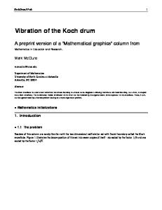
KochDrumPP.nb

Vibration of the Koch drum A preprint version of a “Mathematical graphics” column from Mathematica in Education and Research . Mark McClure [email protected] Department of Mathematics University of North Carolina at Asheville Asheville, NC 28804 Abstract The Koch snowflake is a well known self-similar set whose boundary is a fractal curve. Suppose a vibrating membrane with fixed boundary, i.e. a drum, is shaped like a Koch snowflake. The fundamental modes of vibration of this drum can be modelled by the eigenfunctions of the Laplacian on the snowflake. These, in turn, can be approximated by a discrete problem leading to a matrix eigenvalue problem.

ü Mathematica Initializations

1. Introduction ü 1.1 The problem Readers of this column are surely familiar with the two dimensional self-similar set with fractal boundary called the Koch snowflake. Figure 1 illustrates the decomposition of this set into seven copies of itself - six scaled by the factor 1 ê 3 and one è!!! scaled by the factor 1 ë 3 .

1

KochDrumPP.nb

2

Figure 1: The Koch snowflake Suppose a vibrating membrane with fixed boundary has the shape of a Koch snowflake. What types of vibrational modes are possible? This natural question goes back at least to Berry's work in 1979 [1] and many papers studying the problem have appeared over the years. In the mathematical formulation of the problem, the natural modes of vibrations are described by the eigenfunctions of the Laplacian on the region. Most studies approximate the Koch drum with a discrete grid of points and then translate the problem to a matrix eigenvalue problem. This is the approach taken here using the grid of points recently proposed in [2].

ü 1.2 The plan of attack The basic wave equation is wt t = c2 D w, where wHx, tL is a function of time t and of the spatial variable x restricted to lie in some specified domain. Assuming that wHx, tL = uHxL gHtL and separating variables, we obtain the equations g££ = -lc2 g and D u = -l u. Note that any solution of the equation for u is simply an eigenfunction of the Laplacian on the domain in question and any such u defines a possible shape of the vibration called a fundamental mode. The possible values of l dictate the frequencies of the fundamental modes. For example, if we model the vibration of a string by restricting x to lie in the unit interval, then the equation for u is simply u££ = -l u. We may specify the endpoints as fixed by insisting that uH0L = uH1L = 0. The eigenvalues for this boundary value problem are l = Hn pL2 and the corresponding eigenfunctions are uHxL = sinHn p xL. The leads to the familiar sinusoidal type modes of vibration for a string. For us, of course, x is a two-dimensional variable permitted to range throughout the Koch snowflake and we will assume that wHx, tL = 0 for all x on the boundary of the snowflake. There is no simple analytic formula for the solution and the problem is not amenable to the algorithms incorporated in NDSolve. Thus, we will need to develop our own numerical technique using finite differences based on the approximating grid shown in figure 2. (The different shades of the vertices will be explained shortly.)

KochDrumPP.nb

3

Figure 2: The approximating grid Let x be an interior point of this grid - i.e. an element of the grid and inside the snowflake. Let N denote the set of six nearest neighbors at the distance h from x, possibly including some points outside of the snowflake. Then the Laplacian of a function u at x can be approximated using a second order difference quotient: yz yz 2 ijij D uHxL º ÅÅÅÅÅÅÅÅÅÅÅÅ2Å jjjjjjjj‚ uHyLzzzz - 6 uHxLzzzz. 3h kkyœN { {

Note that formula 0 states that the Laplacian of u at an interior grid point can be approximated with a linear combination of nearby values of u. We would like to eliminate reference to the exterior grid points, called ghost points in [2], and we must enforce the boundary condition. If we view this grid as a graph, then each ghost point is adjacent to precisely one interior grid point. (In this interpretation, however, multiple ghost points can occur at the same location. For example, there are three ghost points at the light vertex near the upper right of figure 2 and each of these are adjacent to a different point in the interior grid.) Now let x be a ghost point and let x£ be the interior point adjacent to x. Symmetry properties of the Laplacian imply that boundary conditions can be enforced by setting uHxL = -uHx£' L. Now since the value at a ghost point is related to the value at its interior neighbor, it is easy to remove reference to the ghost points. To do so, let x be an interior grid point, let N £ denote its set of nearest interior neighbors (not including ghost points), and let n£ = # HN £ L. Then, since each ghost point contributes -uHxL to the sum in formula 0, the approximation may be rewritten 2 jiji zy zy D uHxL º ÅÅÅÅÅÅÅÅÅÅÅÅ2Å jjjjjjjj ‚ uHyLzzzz - H12 - n£ L uHxLzzzz. 3h kkyœN £ { {

This again expresses D uHxL is a linear combination of nearby values of u and uses only interior grid points. Thus formula 0 may be described as multiplication of the vector of values of u at the interior grid points by the appropriate matrix. The eigenvalues of this matrix are approximations to the eigenvalues of the Laplacian and the eigenvectors may be used to approximate the eigenfunctions of the Laplacian. This particular grid was introduced in [2]. Earlier studies, such as [3], used a similar but finer grid which incorporated the vertices of the approximation of the boundary. It is then natural to enforce the boundary condition by simply requiring that uHxL = 0 at these vertices. The authors of [2] report higher accuracy using a larger spacing, thus the technique here might be thought of as more efficient.

KochDrumPP.nb

This particular grid was introduced in [2]. Earlier studies, such as [3], used a similar but finer grid which incorporated the vertices of the approximation of the boundary. It is then natural to enforce the boundary condition by simply requiring that uHxL = 0 at these vertices. The authors of [2] report higher accuracy using a larger spacing, thus the technique here might be thought of as more efficient.

2. Implementation ü 2.1 Setting up the Laplacian approximation We begin by setting up the boundary of the snowflake. The level, boundaryLev, of this approximation is related to, but distinct from, the level of the approximation of the grid of interior points. Both are defined in terms of an overall variable, lev. The boundary is assembled using some fairly standard techniques for the generation of self-similar sets as described in, for example, [4]. lev = 3; boundaryLev = lev + 1; RotationMatrix@t_D := 88Cos@tD, Sin@-tD<, 8Sin@tD, Cos@tD<<; KochStep@8p1_, p2_
We use the self-similarity of the snowflake itself to generate the interior grid. This step is a bit trickier. The snowflake is self-similar consisting of seven copies of itself. More precisely, there are seven functions f0 , f1 , …, f6 that map the snowflake onto the constituent parts shown in figure 1. Take x0 = H0, 0L to be the zeroth level approximation to the interior grid. Any other point in the grid may be realized as fi1 Î fi2 Î Î fin Hx0 L, for some sequence of the fi s. The interior grid is formed by all points generated by such a sequence so that the contraction ratio of fi1 Î fi2 Î Î fin is just smaller than a pre-specified amount, namely 1 ë 3drumLevê2 .

4

KochDrumPP.nb

5

We use the self-similarity of the snowflake itself to generate the interior grid. This step is a bit trickier. The snowflake is self-similar consisting of seven copies of itself. More precisely, there are seven functions f0 , f1 , …, f6 that map the snowflake onto the constituent parts shown in figure 1. Take x0 = H0, 0L to be the zeroth level approximation to the interior grid. Any other point in the grid may be realized as fi1 Î fi2 Î Î fin Hx0 L, for some sequence of the fi s. The interior grid is formed by all points generated by such a sequence so that the contraction ratio of fi1 Î fi2 Î Î fin is just smaller than a pre-specified amount, namely 1 ë 3drumLevê2 . drumLev = 2 lev; RotationMatrix@t_D := 88Cos@tD, Sin@-tD<, 8Sin@tD, Cos@tD<<; è!!!! f0 = 9RotationMatrix@Pi ê 2D ë 3 , 80, 0<=;

A = 881, 0<, 80, 1<< ê 3; ksfIFS = Prepend@Table@8A, 8Cos@tD, Sin@tD<<, 8t, Pi ê 6, 11 Pi ê 6, Pi ê 3 1 ê 3 ^ HdrumLev ê 2L; seqs = First êü Flatten@seqsD; interiorApproxs = FoldList@f, 80., 0.<, #D & êü seqs; interiorGrid = Last êü interiorApproxs; pointPic = ListPlot@interiorGrid, DisplayFunction Ø Identity, PlotJoined Ø FalseD; flakeWithGridPic = Show@ksfPic, pointPicD;

Given a point in this grid, we need quick access to its nearest neighbors in the grid. We can store this information in a nearest neighbor graph, represented as an adjacency matrix, and we can check that we have the correct graph using GraphPlot.

KochDrumPP.nb

dist@h@p_D, h@q_DD := Norm@p - qD; adj = SparseArray@Outer@dist@#1, #2D ã H1.0 ê 3L ^ HHdrumLev - 1L ê 2L &, h êü interiorGrid, h êü interiorGridD ê. 8True Ø 1, False Ø 0
We can now set up the matrix which approximates the Laplacian using formula 0 and compute several eigenvalues. Use of the ShiftØ0 option of the Arnoldi method finds smaller eigenvalues first, rather than larger eigenvalues. This way, we find the lower frequencies first. The scale is the linear scale of size between our Koch drum and the one in [2]; thus, we can compare results. stepSize = H1.0 ê 3L^ HHdrumLev - 1L ê 2L; è!!!! scale = IH3 ê 2L ë I 3 ë 3MM; laplacianRules = Join@8 8i_, i_< ß HTotal@2 adj@@iDDD - 24L ê H3 stepSize ^ 2L<, ArrayRules@adjD ê. H8i_, j_< Ø 1L Ø H8i, j< Ø 2 ê H3 stepSize^ 2LLD; laplacianMatrix = SparseArray@laplacianRulesD; Reverse@Eigenvalues@laplacianMatrix, 10, Method Ø 8"Arnoldi", Shift Ø 0, Tolerance Ø 10-16

These numbers are close to those reported in [2], although the level could be increased to obtain more precise results. The repeated eigenvalues arise due to symmetries between the fundamental modes of vibration.

6

KochDrumPP.nb

7

ü 2.2 Setting up for the graphics Each vibrational mode of the drum may be generated from an eigenvector of our Laplacian matrix, since each component of the vector indicates the relative magnitude of the vibration at a particular point in the interior grid. To set up these graphics, we need to access the individual triangles in our decomposition of the snowflake. Given a vertex in the grid, it is easy to find the triangles containing that vertex, since these are determined by the vertex itself and two of its adjacent vertices. We don't want to do this for every vertex in the interior grid, however, since each triangle would be determined three times. The smaller grid interiorGrid2 has the property that each triangle contains exactly one vertex from interiorGrid2. The points of interiorGrid2 for a lower level decomposition are shaded gray in figure 0. interiorGrid2 = Union@#@@-2DD & êü interiorApproxsD; interiorGrid2Positions = Flatten@Position@interiorGrid, #D & êü interiorGrid2D; adjLists = #@@1, 1DD & êü Most@ArrayRules@#DD & êü adj; triangles@v_D := Module@8pairs<, pairs = Flatten@Table@adjLists@@vDD@@8i, j
We can plot the triangles as a simple check to verify that we've achieved the desired partition. Show@Graphics@MapIndexed@8GrayLevel@Mod@#2@@1DD, 3D ê 3D, Polygon@interiorGrid@@#DDD< & , triangleIndicesDD, AspectRatio Ø AutomaticD;

A glance at figure 0 shows that the snowflake decomposes into a collection of (mostly) triangles together with quadrilaterals near the boundary. Accessing the quadrilaterals is a bit trickier and we will wait until we need to construct the final 3D image to do so.

KochDrumPP.nb

ü 2.3 Generating 3D graphics We still have a bit of work before we can generate 3D images of our Koch drum. One thing we will certainly need is the magnitude of the vibration at each interior grid point. These magnitudes are given by the eigenvectors of the Laplacian matrix. We compute several of those and store one of them to work with. evs = Reverse@Eigenvectors@laplacianMatrix, 10, Method Ø 8"Arnoldi", Shift Ø 0
We now turn our attention to constructing the portion of the drum over the quadrilaterals on the boundary of our decomposed snowflake. We first find the points from the interior grid that have fewer than six neighbors; these are the points nearest to the boundary. The vertices of the quadrilaterals are chosen from these points together with points from the boundary itself, stored in KochVertices. A further complication is the occurrence of two types of quadrilaterals - acute and obtuse. Note that each acute quadrilateral occurs at an acute interior angle of the boundary. Furthermore, the sequence of angles in the boundary occurs in a predictable pattern, which we store in anglePattern. nearBoundaryPositions = Flatten@ Position@Total êü adj, _ ? H# < 6 &LDD; anglePattern = Flatten@Nest@# ê. 8ac Ø 8ac, ob, ac, ob<, ob Ø 8ob, ob, ac, ob<< &, 8ac, ac, ac<, boundaryLevDD;

We can use this to efficiently assemble the quadrilaterals. The individual quadrilaterals will be computed using the functions acuteQuad3D and obtuseQuad3D. acuteQuad3D@n_, ev_D := Module@ 8interiorIndex, oneFudge<, If@n ã 1, oneFudge = -2, oneFudge = n - 1D; interiorIndex = Select@nearBoundaryPositions, Norm@interiorGrid@@#DD - KochVertices@@nDDD < stepSize &D@@1DD; Polygon@8Join@KochVertices@@nDD, 80
We use MapAt in conjunction with the list of angle patterns to construct the right type of quadrilateral at each location. acuteQuads3D = Cases@MapAt@acuteQuad3D@#, evD &, Range@Length@anglePatternDD, Position@anglePattern, acDD, _PolygonD; obtuseQuads3D = Cases@MapAt@obtuseQuad3D@#, evD &, Range@Length@anglePatternDD, Position@Partition@anglePattern, 2, 1D, 8ob, ob
We now proceed in very much the same way that we did when we built our test graphic, but we want to generate 3D polygons incorporating the eigenvector, rather than 2D polygons.

8

KochDrumPP.nb

9

triangle3D@8v1_, v2_, v3_
We can write a function evPlot that incorporates all of these ideas to generate an array of these pictures. Note that evPlot is not stand-alone; it uses much information that we have already computed. Also, evPlot uses EdgeForm[] to suppress the mesh.

KochDrumPP.nb

10

evPlot3D@ev_, opts___D := Module@ 8acuteQuads3D, obtuseQuads3D, allTriangles3D, perim<, acuteQuads3D = Cases@MapAt@acuteQuad3D@#, evD &, Range@Length@anglePatternDD, Position@anglePattern, acDD, _PolygonD; obtuseQuads3D = Cases@MapAt@obtuseQuad3D@#, evD &, Range@Length@anglePatternDD, Position@Partition@anglePattern, 2, 1D, 8ob, ob
References [1] M. Berry, in W. Guttinger and H. Elkheimer, (Eds.) Structural Stability in Physics, Springer-Verlag, Berlin. “Distribution of Modes in Fractal Resonators” (1979) 51–53. [2] J. Neuberger, N. Sieben, and J. Swift, “Computing eigenfunctions on the Koch Snowflake: a new grid and symmetry.” J. Comp. Appl. Math. 191 (2006) 126-142. [3] M. Lapidus, “Fractal drum, inverse spectral problems for elliptic operators and a partial resolution of the Weyl-Berry conjecture.” Trans. Amer. Math. Soc. 325 465-529. [4] M. McClure, “Directed-graph iterated function systems.” Math. Educ. Res. 9 (2000).