VARIATIONAL BHATTACHARYYA DIVERGENCE FOR HIDDEN MARKOV MODELS John R. Hershey, and Peder A. Olsen IBM T. J. Watson Research Center ABSTRACT Many applications require the use of divergence measures between probability distributions. Several of these, such as the KullbackLeibler (KL) divergence and the Bhattacharyya divergence, are tractable for simple distributions such as Gaussians, but are intractable for more complex distributions such as hidden Markov models (HMMs) used in speech recognizers. For tasks related to classification error, the Bhattacharyya divergence is of special importance, due to its relationship with the Bayes error. Here we derive novel variational approximations to the Bhattacharyya divergence for HMMs. Remarkably the variational Bhattacharyya divergence can be computed in a simple closed-form expression for a given sequence length. One of the approximations can even be integrated over all possible sequence lengths in a closed-form expression. We apply the variational Bhattacharyya divergence for HMMs to word confusability, the problem of estimating the probability of mistaking one spoken word for another. Index Terms: Bhattacharyya Error, Bhattacharyya divergence, variational methods, Gaussian mixture models (GMMs), hidden Markov models (HMMs) 1. INTRODUCTION The Bhattacharyya error between two probability density functions f (x) and g(x),[1] � � def 1 B(f, g) = f (x)g(x) dx, (1) 2 is commonly used in statistics as a measure of similarity between two probability distributions. The corresponding Bhattacharyya divergence is defined as DB (f, g) = − log 2B(f, g). The Bhattacharyya divergence has previously been used in machine learning as a kernel [2], and in speech recognition for applications such as phoneme clustering for context dependency trees [3], feature selection [4]. The Bhattacharyya divergence cannot be computed analytically for a pair of mixture models. It can, however, be computed analytically for simple distributions such as gaussians. This makes it possible to come up with some reasonable analytical approximations for mixture models [5, 6]. In this paper, we show how some of these approximations can be directly extended to HMMs. We apply Bhattacharyya divergence to the problem of assigning a score indicating the level of confusability between a pair of spoken words, as in [6, 7], where the words are modeled by HMMs. The Bhattacharyya error satisfies the properties B(f, g) = B(g, f ) (symmetry), B(f, g) = 1/2 if and only if f = g (identification), and 0 ≤ B(f, g) ≤ 1/2 almost everywhere. The Bhattacharyya error is closely related to the Bayes error, Be (f, g) = � 1 min(f (x), g(x)) dx ≤ B(f, g) via the power mean inequal2 ity. The Bhattacharyya divergence is also related to the Kullback-
1-4244-1484-9/08/$25.00 ©2008 IEEE
4557
� Leibler (KL) divergence DKL (f �g) = f (x) log f (x)/g(x) dx ≥ 2DB (f, g), by Jensen’s inequality. For two gaussians f and g the Bhattacharyya divergence has a closed–form expression, [8] 1 DB (fˆ, gˆ) = (μf − μg )� (Σf + Σg )−1 (μf − μg ) 4 � � � Σf + Σ g � 1 1 � − log |Σg Σf | � + log � � 4 2 2
(2)
In fact, the same is true if f and g are any of a wide range of useful distributions known as the exponential family, of which the gaussian is the most famous example. The computation is particularly simple for models with discrete observations. For more complex distributions such as mixture models or hidden Markov models (HMMs), no such closed-form expression exists. Mixture models: We first consider the case where f and g are mixture models, then derive formulas for hidden Markov models. For the sake of concreteness we use gaussian observation distributions, without loss of generality. The marginal densities of x ∈ RD under f and g are thus � f (x) = πa N (x; μa , Σa ) �a (3) g(x) = b ωb N (x; μb , Σb ) where πa is the prior probability of each state, and N (x; μa , Σa ) is a Gaussian in x with mean μa and covariance Σa . We will frequently use the shorthand notation fa (x) = N (x; μa , Σa ) and gb (x) = N (x; μb , Σb ). Our estimates of B(f, g) will make use of the Bhattacharyya error between individual components, which we write as B(fa , gb ). Note that the techniques we introduce apply even if fa (x) and gb (x) are not Gaussians, so long as B(fa , gb ) is known. Hidden Markov models: A hidden Markov model (HMM) can be considered a special case of a GMM in which each state sequence is considered a mixture component. Hence we can in theory apply any approximation that works for a GMM to an HMM. To formulate the Bhattacharyya divergence for hidden Markov models, we must take care to define them in a way that yields a distribution (integrates to one) over all sequence lengths. For an HMM, f , emitting an observation sequence of length n, we let each state a1:n = (a1 , . . . , an ) be a sequence of hidden state discrete random variables, at taking values in E , where E is the set of emitting states. Let x1:n = (x1 , . . . , xn ) be a sequence of observations, with xt ∈ Rd . For the observations we use the shorthand fat (xt ) = N (xt ; μat , Σat ). We also define non-emitting initial and final state values I, and F . The state sequence probabilities � are thus formulated as a Markov chain πa1:n = πa1 |I πF |an n t=2 πat |at−1 , where πa1 |I is an initial distribution, πat |at−1 are transition probabilities, and πF |an are the final state� transitions. The transition probabilities are normalized � such that a1 πa1 |I = 1, and πF |at−1 + at πat |at−1 = 1, for 2 ≤ t ≤ n. For a given sequence length n, we only consider paths
ICASSP 2008
a1:n
�
πa1 |I πF |an fa1 (x1 )
a1:n
n
πat |at−1 fat (xt ),
(5)
t=2
and likewise for g(x1:n ). Note that we can integrate over all se∞ n×d quences � x ∈ ∪n=1 � R � , by summing over sequence lengths; moreover f (x) = ∞ f (x1:n ) dx1:n = 1, so this is a proper denn=1 sity. Because the number of state sequences increases exponentially with the sequence length, and the observation likelihoods at a given time point are shared among many paths, practical computation must invoke an efficient recursion. Unfortunately, the recursion does not directly extend to the Bhattacharyya divergence between two HMMs, where we have to consider all combinations of state sequences. With HMMs, as with GMMs, we can reduce the approximation to pair-wise Gaussian Bhattacharyya divergences. Unless there is a jointly recursive structure in the two HMMs, the approximation will not be tractable.
Jensen Normed Jensen Variational Normed Var. Iterative Var.
2 1.5 1 0.5 0
−1
1
2
3
4
Fig. 1. Distribution of Bhattacharyya approximations relative to MC estimates with 1 million samples, for all pairs of 826 GMMs.
2. VARIATIONAL BOUNDS Variational bounds for mixture models: We can bound the Bhattacharyya error for mixture models using Jensen’s inequality and the concavity of the square root: � � � � 1 1 B(f, g) = fg = πa ωb fa gb (6) 2 2 ab � ˆ jb (f, g). πa ωb B(fa , gb ) = B (7) ≥
2
However, we can improve this bound using variational parameters that express affinities between the states of the two models [6]. Let � φab ≥ 0 satisfy 1 = ab φab . Then by use of Jensen’s inequality we have � � � � 1 πa fa ωb gb 1 B(f, g) = fg = φab (8) 2 2 φab ab � � πa ω b � 1� fa gb φab (9) ≥ 2 φab ab �� φab πa ωb B(fa , gb ). (10) =
Jensen Normed Jensen Variational Normed Var. Iterative Var. Bhatt MC(1M)
1.5 1 0.5 0
−3
×
=
�
n
πa1 |I
a1
×
ab
� a2
4558
πa1 |I πF |an ωb1 |I ωF |bn B 2 (fa1 , gb1 ) πat |at−1 ωbt |bt−1 B 2 (fat , gbt )
t=2
(11)
One problem with this variational method, as well as the simple Jensen bound, is that they fail to preserve the identification property,
2
a1:n b1:n
a� b�
(12)
1
a1:n b1:n
�
=
This bound holds for any φab . Notice that φab = πa ωb , recovers the simple Jensen bound of (6). However, � by maximizing with respect to φab ≥ 0 and the constraint 1 = ab φab we get
which upon substitution into (10) gives
� ˆ vb (f, g). πa ωb B 2 (fa , gb ) = B B(f, g) ≥
0
Variational bounds for hidden Markov models: We extend the bound to HMMs by treating an entire state sequence a1:n as a single state. Thus it is as if we have a variational parameter φa1:n b1:n for each pair of sequences. Fortunately the optimized bound of (12) has a tractable form. Since the variational lower bound sums over the product of the two states πa ωb we can substitute our HMM into this formula and find the recursion. � ˆ vb (f1:n , g1:n )2 = B πa1:n ωb1:n B 2 (fa1:n , gb1:n )
√
πa ωb B (fa , gb ) , πa� ωb� B 2 (fa� , gb� )
−1
Fig. 2. Distribution of Bhattacharyya approximations relative to the Bayes error estimated with 1 million samples, for all pairs of GMMs.
ab
2
−2
Deviation from Bayes divergence MC(1M)
ab
φab = �
0
Deviation from Bhattacharyya divergence MC(1M)
Density
=
ˆ g) = 1/2 if and only if f = g. This can be enforced by that B(f, re-normalizing using the geometric mean of B(f, f ), and B(g, g): ˆnorm (f, g) = B(f, ˆ g)B ˆ −1/2 (f, f )B ˆ −1/2 (g, g). The normalized B estimate is no longer a bound. Nevertheless it is a better approximation, as shown in Figure 1, relative to Monte Carlo estimates, using the variational importance sampling technique proposed in [6]. Surprisingly, the normalization makes the looser Jensen bound perform better than the variational bound. Empirically it also turns out to work better than other power means. Figure 2 shows that in terms of approximating the Bayes error, the normalized Bhattacharyya approximations are almost as good as the Bhattacharyya divergence itself, as estimated using 1 million samples for each pair of 826 GMMs from a speech recognizer. The iterative variational bound shown here is given in [6], and does not need normalization.
Density
that reach the final state after exactly n observations. This allows the HMM to describe a distribution over all sequence lengths. The density assigned to a particular sequence length f (x1:n ) is: � πa1:n fa1:n (x1:n ) (4) f (x1:n ) =
×
� an
� b1
πa2 |a1
ωb1 |I B 2 (fa1 , gb1 )
�
ωb2 |b1 B 2 (fa2 , gb2 ) × . . .
b2
πan |an−1 πF |an
� bn
ωbn |bn−1 ωF |bn B 2 (fan , gbn ). (13)
˜t (at , bt ) as the contriThis can be recursively computed, defining B bution from earlier states to the current estimate at state at , bt . ˜1 (a1 , b1 ) = πa |I ωb |I (14) B 1
1
˜t (at , bt ) = B (15) � � ˜t−1 (at−1 , bt−1 ) πat |at−1 ωbt |bt−1 B 2 (fat−1 , gbt−1 )B at−1
3. WEIGHTED EDIT DISTANCES Various types of weighted edit distances have been applied to the task of estimating spoken word confusability, as discussed in [11] and [12]. A word is modeled in terms of a left–to–right HMM as in Fig. 3. I
bt−1
Handling the end case we get
� � ˆ vb (f1:n , g1:n ) = ˜n (an , bn )B(an , bn ). B πF |an ωF |bn B an
bn
In matrix notation, we write the element-wise product as A ◦ B = {aij bij }, the element-wise exponentiation as A◦n = {an ij }, and the Kronecker product as A ⊗ B = {aij B}. We define transition matrices π = {πat |at−1 } and ω = {ωbt |bt−1 }, and initial and final state probability vectors, πI = {πa1 |I }, ωI = {ωb1 |I }, πF = {πF |an }, ωF = {ωF |bn }, and Bhattacharyya matrices B = {B(fat , gbt )}, ˜t (at , bt )}. The recursion is then ˜ t = {B and B ˜ t−1 ◦ B◦2 )ω ˜ t = π � (B B
˜ t−1 ˜ t = (π ⊗ ω) ◦ ( vec � (B◦2 ) ⊗ 1) vec B vec B
(16)
˜ t−1 , = A vec B � � where A = (π ⊗ ω) ◦ vec � (B◦2 ) ⊗ 1 . Similarly defining vI = πI ⊗ ωI and vF = πF ⊗ ωF , � ˆ vb (f1:n , g1:n ) = B (vF ◦ vec B◦2 )� An vI .
(18)
=
∞ �
ˆ 1:n , g1:n ). B(f
(20)
ˆ 1:n , g1:n ) → 0 as n → ∞, in practice the sum can be Since B(f truncated to the terms that are significantly non-zero. In the case of the Jensen bound, we can compute the whole sum analytically, at the expense of a looser bound. Defining A = (π ⊗ � � ω) ◦ vec � (B) ⊗ 1 , we get
� � ˆ jb (f1:n , g1:n ) = B vF ◦ vec B An vI , (21) Here we can analytically sum over all sequence lengths. Let A = P −1 ΛP be the eigen-decomposition of non-symmetric non-negative � n −1 matrix A. Then ∞ A = P (I − Λ)−1 P − I = (I − A)−1 − n=1 I = C if all eigenvalues are less than one in absolute value, which is guaranteed by the Perron-Frobenius theorem [9]. Hence, ∞ �
(vF ◦ vec B)� An vI
(22)
n=1
= (vF ◦ vec B)� CvI
L
F
Fig. 3. An HMM for call with pronunciation K AO L. In practice, each phoneme is composed of three states, although here they are shown with one state each. The confusion between two words can be heuristically modeled in terms of a cartesian product between the two HMMs as seen in Fig. 4. This structure is similar to that used for acoustic perplexity [11] and the average divergence distance [12]. I
D:K
AY:K
AX:K
L:K
D:AO
AY:AO
AX:AO
L:AO
D:L
AY:L
AX:L
L:L
(19)
n=1
ˆ jb (f, g) = B
AO
(17)
Note that (16) is a more efficient form than (17), taking a factor of K fewer multiplications, where K = |E | is the number of emitting states. However (19) has the nice property that An can be computed using an eigenvalue expansion, which may be much more efficient for longer sequences. Considering all sequence lengths, the approximation is simply ˆ vb (f, g) B
K
(23)
It is possible to extend the tighter iterative variational bound [6] for mixture models to HMMs, by factorizing the variational parameters into a Markov chain, as was done for the KL Divergence in [10]. However this method is more complicated, and models the distribution over pairs of paths less faithfully.
4559
F
Fig. 4. Product HMM for the words call (K AO L) and dial (D AY AX L) In the weighted edit distance (WED), weights are placed on the vertices that assign smaller values when the corresponding phoneme state models are more confusable. The WED is the shortest path (i.e., the Viterbi path) from the initial to the final node in the product graph. [7, 10] DWED (f, g) = min min C(a1:n , b1:n ) n
a1:n ,b1:n
�n
where C(a1:n , b1:n ) = t=1 (wfat |at−1 + wgbt |bt−1 + wfat ,gbt ) is the cost of the path, and the w are costs assigned to each transition. In our experiments we define wfat |at−1 = − log πat |at−1 , and wgbt |bt−1 = − log ωbt |bt−1 . The weight at each node, wfat ,gbt , is a dissimilarity measure between the acoustic models for each pair of HMM states. For the KL divergence WED, we define wfat ,gbt = D(fat �gbt ), and for the Bhattacharyya WED, we define wfat ,gbt = DB (fat �gbt ). An interesting variation, which we call the total weighted edit distance TWED, is to sum over all paths and sequence lengths: � � DTWED (f, g) = − log e−C(a1:n ,b1:n ) . (24) n a1:n ,b1:n
That is, we sum over the probabilities, rather than the costs, which corresponds to the interpretation as a product HMM. The variational vb ˆ vb Bhattacharyya divergence, DB ˆ (f �g) = − log B (f �g), can be
seen as a special case of the total weighted edit distance, with the pairwise Bhattacharyya weights, wfat ,gbt = −2 log B(fat �gbt ). In addition, the TWED with Bhattacharyya weights, wfat ,gbt = jb ˆ jb − log B(fat �gbt ) is identical to DB ˆ (f �g) = − log B (f �g). 4. WORD CONFUSABILITY EXPERIMENTS In this section we describe some experimental results where we use the HMM divergence estimates to approximate spoken word confusability. To measure how well each method can predict recognition errors we used a test suite consisting of spelling data, meaning utterances in which letter sequences are read out, i.e., ”J O N” is read as ”jay oh en.” There were a total of 38,921 instances of the spelling words (the letters A-Z) in the test suite with an average letter error rate of about 19.3%. A total of 7,500 recognition errors were detected. Given the errors we estimated the probability of error for each word pair as E(w1 , w2 ) = 12 P(w1 |w2 ) + 12 P(w2 |w1 ), where P(w1 |w2 ) is the fraction of utterances of w2 that are recognized as w1 . We discarded cases where w1 = w2 , since these dominate the results and exaggerate the performance. We also discarded unreliable cases where the word counts were too low. Continuous speech recognition was used, rather than isolated word recognition, so some recognition errors may have been due to misalignment.
Negative Log Error Rate
6 5 4 3 2 1 0 0
a⋅p a⋅j o⋅r n⋅o e⋅g e⋅t c⋅e e⋅u i⋅ya⋅b i⋅r a⋅n a⋅e c⋅t e⋅pb⋅e l⋅na⋅h p⋅td⋅g d⋅e l⋅m e⋅v g⋅td⋅p a⋅k b⋅d d⋅v v⋅z b⋅pp⋅vf⋅s j⋅kl⋅o d⋅t b⋅v m⋅n
Method MC 100K Min KL Divergence MC 100K Bhattacharyya Divergence KL Divergence Weighted Edit Distance Normalized Bhattacharyya Weighted Edit Distance Normalized VB Bhattacharyya Divergence Normalized JB Bhattacharyya Divergence
Score 0.450 0.530 0.571 0.610 0.631 0.646
Table 1. Squared correlation scores between the various model-based divergence measures and the empirical word confusabilities − log E(w1 , w2 ). VB and JB refer to the variational bound and Jensen bound respectively. Min refers to the min(D(f �g), D(g�f )). MC 100K refers to Monte Carlo simulations with 100,000 samples of HMM sequences. This is natural since the Bhattacharyya divergence is known to yield a tighter bound on the Bayes error than the KL divergence. As with GMMs, the normalized Jensen bound also outperforms the normalized variational bound for HMMs. 5. REFERENCES [1] A. Bhattacharyya, “On a measure of divergence between two statistical populations defined by probability distributions,” Bull. Calcutta Math. Soc., vol. 35, pp. 99–109, 1943. [2] Tony Jebara and Risi Kondor, “Bhattacharyya and expected likelihood kernels,” in Conference on Learning Theory, 2003. [3] Brian Mak and Etienne Barnard, “Phone clustering using the Bhattacharyya distance,” in Proc. ICSLP ’96, Philadelphia, PA, 1996, vol. 4, pp. 2005–2008.
l⋅r
[4] George Saon and Mukund Padmanabhan, “Minimum bayes error feature selection for continuous speech recognition,” in NIPS, 2000, pp. 800–806. [5] John Hershey and Peder Olsen, “Approximating the Kullback Leibler divergence between gaussian mixture models,” in Proceedings of ICASSP 2007, Honolulu, Hawaii, April 2007. [6] Peder Olsen and John Hershey, “Bhattacharyya error and divergence using variational importance sampling,” in Proceedings of Interspeech 2007, August 2007, to appear.
c⋅z 10 20 Divergence Score
[7] Jia-Yu Chen, Peder Olsen, and John Hershey, “Word confusability - measuring hidden Markov model similarity,” in Proceedings of Interspeech 2007, August 2007, to appear.
30
[8] Keinosuke Fukunaga, Statistical Pattern Recognition, Academic Press, Inc., San Diego, CA, 1990.
Fig. 5. The negative log error rate for all spelling word pairs compared to the variational HMM Bhattacharyya score. Figure 5 shows a scatter plot of the variational Bhattacharyya score for each pair of letters, versus the empirical error measurement. Note that similar-sounding combinations of letters appear on the lower left (e.g. ”c·z”), and dissimilar combinations appear in the upper right (e.g. ”a·p”). We computed the divergences by direct Monte-Carlo sampling of the HMM state sequences. In addition to the Bhattacharyya approximations, we also computed KL divergences and a KL divergence weighted edit distance. Table 1 shows the results using all the different methods. The HMM Bhattacharyya divergence approximations outperform all other methods, even the Monte Carlo Bhattacharyya divergence with 100K samples, much to our surprise. Figure 5 shows a scatter-plot of the variational Bhattacharyya score
4560
[9] R.A. Horn and C.R. Johnson, Matrix Analysis, Cambridge University Press, 1990. [10] John R. Hershey, Peder A. Olsen, and Steven J. Rennie, “Variational Kullback Leibler divergence for hidden Markov models,” in Proceedings of ASRU, Kyoto, Japan, December 2007. [11] Harry Printz and Peder Olsen, “Theory and practice of acoustic confusability,” Computer, Speech and Language, vol. 16, pp. 131–164, January 2002. [12] J. Silva and S. Narayanan, “Average divergence distance as a statistical discrimination measure for hidden Markov models,” IEEE Transactions on Audio, Speech, and Language Processing, vol. 14, no. 3, pp. 890–906, May 2006.