PHYSICAL REVIEW B 84, 144420 (2011)
Valence bond entanglement and fluctuations in random singlet phases Huan Tran* and N. E. Bonesteel Department of Physics and National High Magnetic Field Laboratory, Florida State University, Tallahassee, Florida 32310, USA (Received 10 August 2011; published 17 October 2011) The ground state of the uniform antiferromagnetic spin-1/2 Heisenberg chain can be viewed as a strongly fluctuating liquid of valence bonds, while in disordered chains these bonds lock into random singlet states on long-length scales. We show that this phenomenon can be studied numerically, even in the case of weak disorder, by calculating the mean value of the number of valence bonds leaving a block of L contiguous spins (the valence-bond entanglement entropy) as well as the fluctuations in this number. These fluctuations show a clear crossover from a small L regime, in which they behave similar to those of the uniform model, to a large L regime, in which they saturate in a way consistent with the formation of a random singlet state on long-length scales. A scaling analysis of these fluctuations is used to study the dependence on disorder strength of the length scale characterizing the crossover between these two regimes. Results are obtained for a class of models that include, in addition to the spin-1/2 Heisenberg chain, the uniform and disordered critical 1D transverse-field Ising model and chains of interacting non-Abelian anyons. DOI: 10.1103/PhysRevB.84.144420
PACS number(s): 75.10.Pq, 05.10.Ln, 75.10.Nr
I. INTRODUCTION
The set of valence-bond states—states in which localized spin-1/2 particles are correlated in singlet pairs said to be connected by valence bonds—provides a useful basis for visualizing singlet ground states of quantum spin systems. For example, the ground state of the uniform one-dimensional nearest-neighbor spin-1/2 antiferromagnetic (AFM) Heisenberg model (the prototypical spin-liquid state1 ) can be viewed as a strongly fluctuating liquid of valence bonds with a power-law length distribution. This intuitive picture reflects the long-range spin correlations in this state, as well as the existence of gapless excitations created by breaking long bonds. Valence-bond states also play a key role in describing the physics of random spin-1/2 AFM Heisenberg chains. For these systems, it was shown by Fisher,2 using a real space renormalization group (RSRG) analysis, that on long-length scales the ground state is described by a single valence-bond state known as a random singlet state. This single valence-bond state should be viewed as a caricature of the true ground state, which will certainly exhibit bond fluctuations on short-length scales. In fact, it is natural to expect that, when measured on these short-length scales, a fluctuating random singlet state would be difficult to distinguish from the uniform Heisenberg ground state, particularly in the limit of weak disorder. In valence-bond Monte Carlo (VBMC) simulations,3 valence-bond states are used to stochastically sample singlet ground states of quantum spin systems. One of the appealing features of VBMC is that if one imagines viewing the sampled valence-bond states over many Monte Carlo time steps, the resulting “movie” would correspond closely to the intuitive resonating valence bond picture described above. For random Heisenberg chains (and related models) VBMC should therefore provide a useful method for directly studying the phenomenon of random singlet formation on long-length scales, while at the same time capturing the short-range fluctuations, which will always be present. With this motivation, we have carried out a VBMC study of a class of models that include the uniform and random spin1098-0121/2011/84(14)/144420(7)
1/2 AFM Heisenberg chains, as well as models that describe chains of interacting non-Abelian anyons, as special cases. The paper is organized as follows. First, in Sec. II, we define the models and describe their relevant Hilbert spaces. In Sec. III, we give a short review of the VBMC method, and in Sec. IV we present results for the valence-bond entanglement entropy of the uniform and random models. In Sec. V, we introduce the valence-bond fluctuations—a measure of how strongly the valence bonds are fluctuating on a given length scale—and show that this quantity can be used to provide a clear signature of random singlet state formation. Results of a scaling analysis of the valence-bond fluctuations are then presented in Sec. VI, and the paper ends with some conclusions in Sec. VII. II. HILBERT SPACE AND MODEL HAMILTONIANS
To define the class of model Hamiltonians studied here, we first specify the relevant Hilbert spaces on which they act. It is well known that the set of noncrossing valence-bond states [see Fig. 1(a)] forms a complete linearly independent basis spanning the total spin-0 Hilbert space of a chain of spin-1/2 particles.4 We denote the singlet projection operator acting on neighboring sites i and i + 1 by �0i , which, for spin-1/2 particles, can be expressed as �0i =
1 4
− S�i · S�i+1 ,
(1)
where S�i is a spin-1/2 operator (here and throughout h ¯ = 1). Figure 1(b) shows two representative examples of �0i acting on a noncrossing valence-bond state. For spin-1/2 particles, the parameter d appearing in Fig. 1(b) is equal to 2; however, in principle, d can take any value (of course, if d �= 2 the Hilbert space no longer describes spin-1/2 particles). Of particular interest are the cases π , (2) d = 2 cos k+2 where k is a positive integer.5 For these values of d, when k is finite, the noncrossing states are no longer linearly independent and the Hilbert space dimensionality of N sites can be shown
144420-1
©2011 American Physical Society
HUAN TRAN AND N. E. BONESTEEL
PHYSICAL REVIEW B 84, 144420 (2011)
(a)
(b)
Π10
1
2
3
4
=
1
2
3
Π 02
4
1
2
3
4
=
1 d
1
2
3
4
nL = 3
(c)
FIG. 1. (Color online) (a) A noncrossing valence-bond state. (b) Action of singlet projection operators �0i on a noncrossing valence-bond state. (c) A noncrossing valence-bond state with a block of L = 5 sites (region enclosed in the box) for which nL , the number of bonds leaving the block, is 3.
to grow asymptotically as d N with d < 2. The k → ∞ limit then corresponds to the case of ordinary spin-1/2 particles with d = 2 for which the Hilbert space dimensionality grows as 2N . One consequence of the reduced Hilbert space dimensionality for finite integer k is that it changes the entanglement entropy associated with a valence bond. The entanglement entropy of a subsystem A of a larger system consisting of parts A and B is defined to be the von Neumann entropy, S vN , of the reduced density matrix ρA obtained by tracing out the degrees of freedom in region B, thus S vN = −Tr[ρA log2 ρA ].
(3)
With this definition, an ordinary singlet formed by two spin1/2 particles, with one spin in region A and the other in region π , it was B, will have S vN = 1. However, when d = 2 cos k+2 shown in Ref. 6 that if there are M valence bonds connecting sites in region A with sites in region B, then, in the M � 1 limit, because the dimensionality of the traced out Hilbert space grows as d M , S vN � M log2 d and the entanglement per bond is log2 d. The class of Hamiltonians studied here are all characterized by the parameter d and have the form � Ji �0i , (4) H =−
conformally invariant 1+1 dimensional systems11 implies that the entanglement entropy of a block of L contiguous sites, SLvN , in the ground states of these models will scale logarithmically for L � 1 as10 ck log2 L. SLvN � (5) 3 When the Ji are random, the Hamiltonians (4) can no longer 2 be solved exactly. However, the RSRG approach √ of Fisher can be straightforwardly applied for all d � 2 with the result that the ground states all flow to the same infinite randomness fixed point6,12 —one for which the bond strength distribution is the same as that of the fixed point of the random Heisenberg chain.2 For this fixed point, Refael and Moore13 have shown that if nL is the number of valence bonds leaving a given block of size L [see Fig. 1(c)], then, in the L � 1 limit, ln L ln 2 (6) � log2 L, 3 3 where the overbar denotes a disorder average over random singlet states produced by the RSRG. This logarithmic scaling is a direct consequence of the inverse-square distribution of valence bond lengths characteristic of random singlet states.14 Multiplying nL by the entanglement per bond of log2 d then yields the RSRG result for the asymptotic scaling of the entanglement entropy for the random ABF models, which is again logarithmic and has the form6,13 nL �
SLvN � nL log2 d �
(7)
III. VALENCE-BOND MONTE CARLO
When applying the VBMC method3 to Hamiltonians of the form (4), the ground state is projected out by repeatedly applying −H to a particular noncrossing valence-bond state |S . The result of this projection after n iterations is � (−H )n |S = Ji1 · · · Jin �0i1 · · · �0in |S . (8) i1 ,···,in
i
with Ji > 0. For d = 2, these models correspond to spin-1/2 AFM Heisenberg chains with Ji equal to the exchange energy associated with spins i and i + 1. For general d, if the Ji are uniform (Ji = J ) the Hamiltonians (4) can be viewed as 1+1 dimensional quantum Potts models obtained by taking the asymmetric limit of the transfer matrix of the Q-state Potts models7 with Q = d 2 . For d � 2, the uniform models are all gapless, and for the π special values d = 2 cos k+2 they correspond to a sequence of conformally invariant Andrews-Baxter-Forrester8 (ABF) models with central charges ck = 1 − 6/(k + 1)(k + 2).9 Physically, these ABF models can be thought of as describing chains of interacting non-Abelian particles described by su(2)k Chern-Simons-Witten theory, believed to be relevant 10 for certain quantum Hall √ states. Two special cases of these models are k = 2 (d = 2), which corresponds to the critical 1D transverse field Ising model, and k = 3 (d = φ where √ φ = ( 5 + 1)/2 is the golden mean), which corresponds to the so-called golden chain made up of interacting Fibonacci anyons.10 The known universal entanglement scaling of
ln d log2 L. 3
The properties of the projection operators shown in Fig. 1(b) imply that �0i1 · · · �0in |S = λi1 ,···,in |α , where |α is a noncrossing valence-bond state with the same norm as |S . The coefficient is given by λi1 ,···,in = d −m , where m is the number of times a projection operator acts on two sites that are not connected by a valence bond when projecting |S onto |α .3,15 This projection thus leads to an expression for the ground state |ψ , which becomes exact in the limit of large n (in our simulations we find it is sufficient to take n = 60N , where N is the number of sites) and has the form � |ψ = w(α)|α , (9) α
where w(α) = Ji1 · · · Jin λi1 ···in . In the simplest form of VBMC, the valence-bond states |α contributing to |ψ are sampled with probability w(α) by updating the sequence of projection operators (i1 , · · · ,in ) using the usual Metropolis method.3 To use VBMC to calculate the quantum mechanical expectation value of given operator O, i.e., ψ|O|ψ / ψ|ψ , it is necessary to project the ground state out of both the bra and ket states, in which case one samples from
144420-2
VALENCE BOND ENTANGLEMENT AND FLUCTUATIONS IN . . .
for any state |ψ of the form of Eq. (9), provided w(α) � 0. In what follows, angle brackets will always denote this average, though it should be noted that O will in general not be equal to ψ|O|ψ / ψ|ψ , both because the valence-bond states are nonorthogonal and because the weight factors w(α) are amplitudes and not probabilities. IV. VALENCE-BOND ENTANGLEMENT
One quantity that can be calculated naturally by VBMC is the valence-bond entanglement entropy, SLVB , which, for the uniform Heisenberg chain, is defined to be equal to nL , the average number of valence bonds leaving a block of size L.16,17 π To generalize SLVB to the ABF models with d = 2 cos k+2 , it is natural to multiply nL by the asymptotic entanglement per bond of log2 d. For this choice, provided nL � 1, SLVB will be equal to SLvN for any single valence-bond state. We therefore take SLVB = nL log2 d.
(11)
While SLVB is easy to compute numerically by VBMC, for a general superposition of valence-bond states it will not be equal to SLvN . Nonetheless, VBMC simulations16–18 of the uniform AFM Heisenberg chain with N � 100 spins have shown numerically that SLVB grows logarithmically with L, in the same fashion as the von Neumann entanglement SLvN . To characterize this log scaling it is convenient to introduce an effective valence-bond central charge, cVB , defined so that SLVB �
cVB log2 L, 3
(12)
in the limit L � 1. In addition to showing log scaling of SLVB , previous VBMC simulations of the uniform AFM spin-1/2 Heisenberg chain have given results consistent with cVB being close to,17 or even possibly equal to,16 1, the value of the true central charge for the uniform d = 2 model. However, Jacobsen and Saleur19 were able to determine the exact asymptotic scaling of nL analytically for all d � 2. Their results both confirmed the log scaling of SLVB for L � 1 and provided an analytic result for the coefficient of the log, which yields the following expression for the valence-bond central charge, � 6 ln d 2 + d arccos(d/2) . (13) cVB = π 2 − d π − arccos(d/2)
4.0 Uniform
k→ ∞
SL
VB
3.0
k=3
2.0
k=2
1.0 0.0 3.0
SLVB
“loop” configurations corresponding to the valence-bond state overlaps α|β with probabilities weighted by w(α)w(β).3 However, using the “one-way” VBMC described above in which one simply samples from the valence-bond basis it is possible to calculate a number of interesting quantities that can be used to characterize the intuitive valence-bond description of the ground-state wavefunction. In particular, given an observable O with expectation values O(α) = α|O|α / α|α in the noncrossing valencebond states |α , VBMC can be used to compute the average � w(α)O(α) , (10)
O = α� α w(α)
PHYSICAL REVIEW B 84, 144420 (2011)
Random
k→ ∞
2.0
k=3 k=2
1.0 0.0
1
10
100
600
LC FIG. 2. (Color online) Log-linear plots of valence-bond entanglement SLVB as a function of conformal distance LC = (N/π ) sin(Lπ/N ) for uniform (upper panel) and random (lower panel) models with k = 2,3, and ∞. For uniform models, the solid lines correspond to the exact asymptotic scaling, which follows from Ref. 19. For random models, the solid lines show the asymptotic scaling predicted by the RSRG.13 Results are for periodic chains with N = 1024 sites. For random chains, we take the disorder strength to be u = 1 [see Eq. (14)] and results are self-averaged over all blocks for 50 disorder samples.
In the limit d → 2, this expression gives cVB = 12 ln 2/π 2 � 0.843, which is therefore not equal to the true central charge of 1. VB Figure 2(a) shows our VBMC √ results for SL for k = 2,3, and ∞ (corresponding to d = 2,φ and 2, respectively) for periodic systems with N = 1024 sites. To minimize finite size effects when L is comparable to N/2, SLVB is plotted as a function of the conformal distance LC = (N/π ) sin(π L/N ). The solid lines show the exact asymptotic scaling found by Jacobsen and Saleur,19 which clearly agree with our numerical results for L � 1. Note that for the case k → ∞, it is necessary to consider fairly large values of L before entering the scaling regime, whereas for k = 2 and 3, the scaling begins at relatively small L. This fact may account for the initial numerical difficulty in determining cVB for d = 2 using small systems (see, however, Ref. 18). Presumably, the reason that the finite-size effects become more pronounced as d approaches 2 is because this is a critical value (for d > 2 the uniform models acquire a gap7 ). For random Heisenberg chains, SLVB was first computed numerically by Alet et al.16 Following the same procedure as these authors, we compute SLVB by determining nL for particular realizations of disorder and then disorder averaging. Throughout this paper we assume the random models are characterized by a flat bond strength distribution centered around J = 1 of width u,
144420-3
P (J ) =
1
[(1 + u) − J ] [J − (1 − u)], 2u
(14)
HUAN TRAN AND N. E. BONESTEEL
PHYSICAL REVIEW B 84, 144420 (2011)
where u is a measure of disorder strength. For the random ABF models, we again multiply nL by the entanglement per bond, and thus take
the uniform case, becomes independent of d when disorder is included. V. VALENCE-BOND FLUCTUATIONS
SLVB = nL log2 d,
(15)
(here again the overbar denotes disorder average). Figure 2(b) shows log plots of our results for SLVB for random chains with strong disorder (u = 1), again for k = 2,3, and ∞ and N = 1024. The solid lines show the scaling predictions based on the RSRG6,13 for SLvN , which clearly agree with our numerical results. As pointed out by Alet et al.,16 the fact that SLVB and SLvN show the same scaling for L � 1 is to be expected if, as predicted by the RSRG, on long-length scales the ground states of the random models are dominated by a single valence-bond configuration. The log scalings of SLVB shown in Figs. 2(a) and 2(b) are summarized in Fig. 3, which shows our VBMC results for cVB for both uniform and random models and various values of d corresponding to k → ∞ and k = 2,3,4,5,6. For the uniform models, Fig. 3 also shows the exact values of cVB [see Eq. (13)], which follow from the analytic results of Jacobsen and Saleur19 as well as the true central charges ck of the π 20 ABF models with d = 2 cos k+2 . For the random models, VB the d dependence of c is seen to be entirely due to the entanglement per bond, reflecting the fact that the valence bond length distribution, which determines the coefficient in front of the log scaling of nL , and which depends on d for 1.1
1.0
The expectation that for random models the L � 1 scaling of SLVB should be the same as that of SLvN is based on the assumption that the valence bonds in the ground state of the model lock into a particular random singlet configuration on long-length scales. This assumption is in turn based on the RSRG approach which, although it can be shown to capture the long distance properties of the fixed point exactly,2 is still an approximate method. Consequently, it is clearly desirable to have a direct numerical demonstration that the valence bonds are indeed locking into a particular random singlet configuration on long length scales. To provide such a demonstration, we calculate the fluctuations in nL , a quantity we refer to as the valence-bond fluctuations. To be precise, we first compute the quantity
n2L − nL 2 for a particular block of size L and a particular realization of disorder, and then perform a disorder average. The quantity we compute is thus � � σL2 = n2L − nL 2 . (16) For this choice of averaging σL2 has the property that, in an idealized random singlet phase for which the ground state is precisely a single noncrossing valence-bond state, σL2 would vanish, even though the number of bonds leaving a given block would be different for different realizations of disorder. For the uniform models with d � 2, Jacobsen and Saleur19 have also determined the asymptotic scaling of σL2 (in this case there is, of course, no disorder average). Like nL , σL2 scales logarithmically with L for L � 1, with σL2 � b ln L,
c / log2d
1.2
0.9
1.1
c
VB
0.8
k→ ∞
0.9 0.8
and the analytic results of Ref. 19 can again be used to obtain an exact analytic results for the coefficient, b, as a function of d, � √ 2 + d 2 arccos(d/2) − 4 − d 2 4 . (18) b= π (2 − d)3 π − arccos(d/2)
k=2
1.0
N 0.00
0.02
0.04
−1/2
0.06
0.08
0.7 1.4
1.5
1.6
1.7
(17)
1.8
1.9
2
d FIG. 3. (Color online) d dependence of the valence-bond central charge, cVB , for uniform and random chains, along with the true central charges for the conformally invariant uniform models with π , in units of log2 d—the entanglement per bond. The d = 2 cos k+2 solid red line is the exact result of Jacobsen and Saleur19 for nL π ) vs. d for uniform (which equals cVB / log2 d when d = 2 cos k+2 models, the black squares are the central charges of the ABF models for different values of k (the dashed line is a guide to the eye), the black line is the RSRG result cVB / log2 d = ln 2 for the random models, and the blue symbols are our VBMC results for uniform and random models. The inset shows the finite-size extrapolation used to find cVB for the uniform models with k → ∞ and k = 2. The extrapolation clearly show the strong finite-size effects for the k → ∞ case with d = 2.
Figure 4 shows a log-linear plot of our VBMC results for σL2 calculated for the uniform model with k → ∞. A line corresponding to the exact asymptotic log scaling found by Jacobsen and Saleur19 is also shown. It is readily seen that our numerical results agree well with the predicted asymptotic scaling and can be regarded as further numerical confirmation of the field-theoretic analysis of Ref. 19. We note that the log scaling of σL2 directly demonstrates the existence of bond fluctuations on all length scales in the ground state of the uniform model. Figure 4 also shows that for small L the valence-bond fluctuations σL2 oscillate strongly as the block length L changes from even to odd. The origin of this even/odd effect can be understood by first considering a state in which the bonds are all of length 1 (i.e., a dimerized state). In this case there would be two ground states corresponding to the two distinct dimerizations and the translationally invariant ground state would be an equal superposition of these two dimerized
144420-4
VALENCE BOND ENTANGLEMENT AND FLUCTUATIONS IN . . .
PHYSICAL REVIEW B 84, 144420 (2011) 2.5
2.5
k→ ∞
u=0.00
2.0
2.0
σL2
σL
2
u=0.25
1.5
u=0.50
1.5
u=0.75
1.0
u=1.00
1.0 0.5
0.5
2.5
0.0
k=3
u=0.00 u=0.25
100
600
LC FIG. 4. (Color online) Log-linear plot of the valence-bond fluctuations σL2 as functions of the conformal distance LC = (N/π ) sin(Lπ/N ) for the case k → ∞. The exact log scaling obtained by Jacobsen and Saleur is shown by the solid line. For small L, a strong even/odd effect—explained in the text—can be seen. Here and throughout values for σL2 were computed for all values of L up to L = 30, and then for L equal to multiples of 15 for L > 30. Results are for periodic chains with N = 1024 sites.
u=0.50
1.5
u=0.75 u=1.00
1.0 0.5 2.5
u=0.00
k=2
u=0.25
2.0
σL2
10
σL2
2.0
1
u=0.50 u=0.75
1.5
u=1.00
1.0
states. One can readily check that in such a state σL2 = 1 when L is even, and σL2 = 0 when L is odd. We believe that the even/odd oscillations apparent in Fig. 4 for small L are due to the significant contribution of such dimerized regions (at least on small length scales) to the ground state wavefunction. For random models, the RSRG approach2 shows that on long-length scales the bonds lock into a random singlet state. At the same time, on short-length scales (if disorder is weak) it is natural to expect that the bonds will fluctuate strongly, as they do in the uniform models. This implies the existence of crossover-length scale ξ , which characterizes the transition from the uniform regime to the random-singlet regime of these models with increasing L. One can then expect the valence-bond fluctuations σL2 to not differ much from their value for the uniform models when L � ξ , but for L � ξ the fluctuations σL2 should saturate. This saturation is due to the fact that, once the block size L becomes much larger than the crossover-length ξ , the bond fluctuations occurring outside of a distance ξ from the two boundaries of the block will not change the number of bonds leaving the block and hence will not contribute to the valence-bond fluctuations. Figure 5 shows log-linear plots of our results for σL2 for the case k → ∞ (corresponding to the Heisenberg chain, with d = 2), k = 3 (corresponding to the golden chain, with d = φ), and k = 2 (corresponding to the critical transverse √ field Ising model, with d = 2) for both uniform and random models. For the random models, the Ji are taken to be distributed according to Eq. (14), where u is a measure of disorder strength. It can be observed from Fig. 5 that the valence-bond fluctuations σL2 for the random models saturates, regardless of how weak the disorder is, on a finite-length scale ξ , which grows as u decreases. The observation of this saturation, which indicates a finite crossover-length scale ξ beyond which the valence bonds
0.5 1
10
100
700
LC FIG. 5. (Color online) Log-linear plots of valence-bond fluctuations as a function of conformal distance LC = (N/π ) sin(Lπ/N ), for both uniform and random chains for k → ∞ (upper panel), k = 3 (middle panel), and k = 2 (lower panel). For uniform chains, these fluctuations grow logarithmically with LC in agreement with the analytic results of Ref. 19 (solid red lines), indicating that bonds are strongly fluctuating on all length scales. For random chains the fluctuations saturate beyond a given finite length scale ξ , signaling the formation of a random singlet phase in which the bonds have locked into a particular random singlet configuration on long-length scales. The parameter u (defined in the text) is a measure of the disorder strength and the results clearly show that the saturation-length scale grows with decreasing u. Results are for periodic chains with N = 1024 sites and for random models are self-averaged over all blocks for 100 disorder samples.
effectively lock into a random singlet configuration, together with the log scaling of nL , which indicates a power-law distribution of valence bond lengths, provides a direct numerical proof of random singlet phase formation in these models. VI. CROSSOVER LENGTH SCALE
As described in the previous section, the saturation of σL2 with increasing L for disorder of any strength u implies the existence of a finite fluctuation-length scale ξ , which characterizes the transition from the resonating regime with L � ξ to the saturation regime with L � ξ . This length scale ξ is essentially the crossover-length scale from the uniform regime to the disordered regime, which has been studied in the literature both analytically and numerically for a number of models.21–24
144420-5
HUAN TRAN AND N. E. BONESTEEL
PHYSICAL REVIEW B 84, 144420 (2011)
For k → ∞ and k = 2, analytic results for the dependence of ξ on u can be obtained for the case of weak disorder21 by mapping the model (4) onto disordered Luttinger liquids.22 For k → ∞, the model (4) corresponds to an isotropic spin-1/2 Heisenberg chain that, via a Jordan-Wigner transformation, can be mapped onto a 1D interacting spinless Fermi gas with a particular interaction strength. Similarly, for the case k = 2, the model (4) corresponds to the 1D transverse field Ising model, and a pair of independent but identical 1D transverse field Ising models can be mapped onto a spin-1/2 XX model, which can in turn be mapped onto a (in this case free) 1D spinless Fermi gas. The resulting predictions21,22 for the scaling of the crossover-length scale ξ with disorder strength u for these two cases are that ξ ∼ u−1 for k → ∞ and ξ ∼ u−2 for k = 2. Numerical results for ξ , based on scaling analyses of the spin-spin correlation function23,24 and the spin stiffness24 of the Heisenberg chain (using quantum Monte Carlo) and 0.1 0.0
ξ
k→ ∞
2
σ L - σ2 ∞
-0.1
102
u = 1.000 u = 0.750 u = 0.625 u = 0.500 u = 0.375 u = 0.250
-0.2 -0.3 -0.4 -0.5
−1.00
∼u
1
-0.6 0.1 0.0
k→ ∞
10 k=3
3
ξ
k=3
10
2
-0.2
2
σ L-σ ∞
-0.1
-0.3
u = 1.000 u = 0.750 u = 0.625 u = 0.500 u = 0.375 u = 0.250
-0.4
102
-0.5
0.0
ξ
k=2
10
2
u = 1.000 u = 0.750 u = 0.625 u = 0.500 u = 0.375 u = 0.250
-0.2 -0.3 -0.4
2
10
-0.5 -0.6 10-1
k=2
3
-0.1
σ2L - σ ∞
∼ u−1.55
101
-0.6 0.1
−1.80
0
10
LC / ξ
1
10
101
∼u 0.1
1.0
u
FIG. 6. (Color online) (Left) Scaling plots of the valence-bond 2 2 subtracted out), σL2 − σ∞ , fluctuations (with the saturation value σ∞ for k → ∞, k = 3, and k = 2 and various disorder strengths u. In these plots, the x axes are rescaled by choosing the disorder-dependent crossover length ξ so that the data for different u collapse onto a single curve when plotted vs. LC /ξ , where LC = (N/π ) sin(Lπ/N ). The solid lines show the predicted log scaling for the uniform models.19 The values of ξ determined by this scaling procedure are summarized on Table I. (Right) Log-log plots of the crossover-length scale ξ as a function of u for k → ∞, k = 3, and k = 2. Solid lines represent the power-law scaling determined from the data: ξ ∼ u−1 for k → ∞, ξ ∼ u−1.55 for k = 3, and ξ ∼ u−1.8 for k = 2.
the XX chain (by exact diagonalization) have shown results consistent with these weak disorder renormalization group predictions. It is possible to determine the dependence of ξ on u by performing a scaling analysis of the valence-bond fluctuations σL2 . To do this, we first subtract the large L saturated value of 2 ) obtained by extrapolating the fluctuations (limL→∞ σL2 = σ∞ the data shown in Fig. 5 and attempt to collapse the data by assuming a scaling function f and a u-dependent ξ for which � LC 2 σL2 (u) − σ∞ . (19) (u) = f ξ (u) 2 For each value of u, ξ (u) is chosen so that data for σL2 − σ∞ collapse onto a single curve, with the center of the crossover regime being LC /ξ � 1. Note that to avoid the even-odd effect pointed out earlier for small L we only use odd values of L, and to minimize finite-size effects for large L we use the conformal distance LC in the scaling analysis. Results of carrying out this analysis for the cases k → ∞, k = 3, and k = 2 are shown on the left side of Fig. 6. The 2 VBMC results for σL2 − σ∞ can be seen to be well collapsed onto a particular scaling function f (LC /ξ ), according to the definition Eq. (19). The values we obtain for ξ for these models corresponding to various disorder strength u are given in Table I. On the right side of Fig. 6, log-log plots of the crossoverlength scales ξ as a function of the disorder strength u are shown. The exponents characterizing the divergence of ξ are determined by fitting the data to the power law u−η (solid lines). For k → ∞, we find η � 1, consistent with the weak-disorder renormalization group prediction21,22 of η = 1. For k = 2, we find η � 1.8, which is somewhat less than the predicted value of η = 2. One possible reason for the poorer agreement in this case is that for k = 2, the length scale ξ is significantly larger than for k → ∞ for a given disorder strength, and it may therefore be necessary to study larger system sizes in order to enter the scaling regime for the valence-bond fluctuations. For the case k = 3, for which the model (4) corresponds to a disordered golden chain, we find the exponent η � 1.55. Note that for this system (with d = φ), and, in fact, for all cases for √ which d �= 2, 2, there is no simple mapping of Hamiltonian (4) to a disordered 1D Luttinger liquid. It is therefore not possible to apply the same weak-disorder renormalization group analysis to these models that√can be used to obtain the exponent η for d = 2 and d = 2. To the best of our
TABLE I. Crossover-length scale ξ extracted from the scaling analysis of the valence-bond fluctuations σL2 for different disorder strengths u for k → ∞, k = 3, k = 2. u 0.250 0.375 0.500 0.625 0.750 1.000
144420-6
k→∞
k=3
70 51 37 29 21 11
215 145 87 65 48 24
k=2 390 195 140 102 66 32
VALENCE BOND ENTANGLEMENT AND FLUCTUATIONS IN . . .
knowledge, there are no known analytic results for η or for these more general models, and we believe our result for k = 3 represents the first numerical calculation of such an exponent. VII. CONCLUSIONS
In this paper, we have presented the results of a VBMC study of both uniform and random Hamiltonians of the form (4). Both the valence-bond entanglement entropy SLVB and the valence-bond fluctuations σL2 were calculated for these models. For uniform models, both these quantities were found to scale logarithmically with L and our results agreed well with analytic results obtained through a field-theoretic analysis by Jacobsen and Saleur.19 For random models, SLVB was also found to scale logarithmically with L, consistent with predictions based on the RSRG,6,13 while σL2 was found to saturate once L exceeded a disorder-dependent crossover-length scale ξ , signaling the expected locking of the valence bonds into a particular random singlet configuration on long length scales. By performing a scaling analysis of the valence-bond fluctuations, we were able to determine the dependence of ξ on
*
Current address: Department of Physics, University of Basel, Klingelbergstrasse 82, 4056 Basel, Switzerland 1 P. W. Anderson, Science 235, 1196 (1987). 2 D. S. Fisher, Phys. Rev. B 50, 3799 (1994). 3 A. W. Sandvik, Phys. Rev. Lett. 95, 207203 (2005). 4 G. Rumer, G¨ottingen Nachr. Tech. 1932, 377 (1932). 5 See, for example, L. H. Kaufmann and S. L. Lins, TemperleyLieb Recoupling Theory and Invariants of 3-Manifolds (Princeton University Press, Princeton, NJ, 1994). 6 N. E. Bonesteel and K. Yang, Phys. Rev. Lett. 99, 140405 (2007). 7 P. P. Martin, Potts Models and Related Problems in Statistical Mechanics (World Scientific, Singapore, 1991). 8 G. E. Andrews, R. J. Baxter, and P. J. Forrester, J. Stat. Phys. 35, 193 (1984). 9 D. A. Huse, Phys. Rev. B 30, 3908 (1984). 10 A. Feiguin, S. Trebst, A. W. W. Ludwig, M. Troyer, A. Kitaev, Z. Wang, and M. H. Freedman, Phys. Rev. Lett. 98, 160409 (2007). 11 C. Holzhey, F. Larsen, and F. Wilczek, Nucl. Phys. B 424, 443 (1994); G. Vidal, J. I. Latorre, E. Rico, and A. Kitaev, Phys. Rev. Lett. 90, 227902 (2003). 12 When ferromagnetic bonds (Ji < 0) are allowed the behavior of the models becomes much richer and the random models flow to
PHYSICAL REVIEW B 84, 144420 (2011)
disorder strength. For the cases k → ∞ (spin-1/2 Heisenberg model) and k = 2 (transverse field Ising model), our results were consistent with those based on a weak-disorder renormalization group approach21,22 as well as previous numerical work,23,24 although for the case k = 2, we may not have fully entered the scaling regime. An appealing feature of our bond-fluctuation-based approach is that it can be used to determine ξ for any value of k, not just k → ∞ and k = 2 for which the model (4) can be mapped onto 1D Luttinger liquids (the starting point for the weak-disorder renormalization group approach). For example, we have determined for the first time the crossover length scale ξ and the corresponding exponent η � 1.55 for the model (4) with k = 3, which corresponds to the disordered golden chain. ACKNOWLEDGMENTS
This work was supported by US DOE Grant No. DEFG02-97ER45639. The authors thank K. Yang, A. Sandvik, P. Henelius, J. A. Hoyos, and F. Alet for useful discussions. Computational work was performed at the Florida State University High Performance Computing Center.
different fixed points which depend on k; see L. Fidkowski, H. H. Lin, P. Titum, and G. Refael, Phys. Rev. B 79, 155120 (2009). 13 G. Refael and J. E. Moore, Phys. Rev. Lett. 93, 260602 (2004). 14 J. A. Hoyos, A. P. Vieira, N. Laflorencie, and E. Miranda, Phys. Rev. B 76, 174425 (2007). 15 H. Tran and N. E. Bonesteel, Comput. Matter. Sci. 49, S395 (2010). 16 F. Alet, S. Capponi, N. Laflorencie, and M. Mambrini, Phys. Rev. Lett. 99, 117204 (2007). 17 R. W. Chhajlany, P. Tomczak, and A. W´ojcik, Phys. Rev. Lett. 99, 167204 (2007). 18 A. B. Kallin, I. Gonzalez, M. B. Hastings, and R. G. Melko, Phys. Rev. Lett. 103, 117203 (2009). 19 J. L. Jacobsen and H. Saleur, Phys. Rev. Lett. 100, 087205 (2008). 20 It is interesting to note that while cVB and ck are not equal for the uniform ABF models, they are close in magnitude. This is primarily due to the fact that the entanglement per bond, log2 d, is equal to ck for k = 2 and k → ∞, and very close to ck for k > 2. 21 C. A. Doty and D. S. Fisher, Phys. Rev. B 45, 2167 (1992). 22 T. Giamarchi and H. J. Schulz, Phys. Rev. B 37, 325 (1988). 23 N. Laflorencie and H. Rieger, Eur. Phys. J. B 40, 201 (2004). 24 N. Laflorencie, H. Rieger, A. W. Sandvik, and P. Henelius, Phys. Rev. B 70, 054430 (2004).
144420-7