Uniform generation of random directed graphs with prescribed degree sequence Diploma Thesis
Petko P. Fiziev Department of Mathematics and Computer Science Institute of Computer Science Free University of Berlin, Germany
Advisor: Prof. Martin Vingron Computational Molecular Biology Department Max Planck Institute for Molecular Genetics, Berlin, Germany
March 31, 2006
CONTENTS
1. Introduction . . . . . . . . . . . . . . . . . . . . . . . . . . . . . . .
2
2. Methods . . . . . . . . . . . . . . . . . . . . 2.1 The Switching Algorithm . . . . . . . . 2.2 The Matching Algorithm . . . . . . . . 2.3 The ”Go with the Winners” Algorithm
. . . .
. . . .
. . . .
. . . .
. . . .
. . . .
. . . .
. . . .
. . . .
. . . .
. . . .
. . . .
. 5 . 6 . 17 . 27
3. Results . . . . . . . . . . . . . . . . . . . . . 3.1 The Switching Algorithm . . . . . . . . 3.2 The Matching Algorithm . . . . . . . . 3.3 The ”Go with the Winners” Algorithm
. . . .
. . . .
. . . .
. . . .
. . . .
. . . .
. . . .
. . . .
. . . .
. . . .
. . . .
. . . .
. . . .
33 33 35 37
4. Discussion . . . . . . . . . . . . . . . . . . . . . . . . . . . . . . . . 39 5. Summary . . . . . . . . . . . . . . . . . . . . . . . . . . . . . . . . 42 6. Acknowledgements . . . . . . . . . . . . . . . . . . . . . . . . . . . 43
To my father.
1. INTRODUCTION Directed graphs (digraphs) are a mathematical abstraction for binary relations. One can visualize them on a piece of paper by drawing dots connected with arrows. Each dot represents an object from a given universe of discourse and each arrow means that the two objects that are source and target of it belong as a tuple to the relation. In graph theory the dots are called vertices and the arrows - edges. A directed graph G is defined as the tuple (V, E), where V is the set of all vertices and E is the set of all edges in it. Many problems in fields ranging from economics to molecular biology can be formulated in the terms of graph theory. It is interesting then to analyze the properties of the graphs and draw conclusions about the world that they model. One of the most tempting questions is the one about the origin of the relation. Does it result from a natural evolution-like process or was it designed specifically for the task? Some networks that arise by the hands of humans are designed; probably the best known example are electronic circuits. If displayed correctly one can tell only with a naked eye flip-flops from multiplexers, adders from multipliers and so on in a graph that represents the connections between transistors in a microprocessor chip, if one knows how a single flip-flop or a multiplier looks like. On the other hand, there are many networks that arise by a process that is a mixture between evolution and design like public transport or the internet. Clearly, there is some design involved here. For example, in public transport there are often cycles and long bidirectional lines that cross each other. On the other hand, it is always adapted by shortcuts to things of local importance like banks, governmental buildings, museums, airports and so on. It is hard to say, whether there will be ever a network that models some human activity and does not show any signs of design. Nevertheless, the same does not necessarily apply to graphs that represent natural processes in life on low level like signal transduction, metabolic pathways, gene regulation, protein-protein interactions, neuron connectivity in brain and many more. It is tempting to say that there was design in them, but to prove it might be far from easy. Research in this direction has started some years ago. A well known example is the discovery that a three-node structure called ”feedforward” loop (FFL) occurs statistically more often in the network of
1. Introduction
3
transcriptional regulation in the bacteria E.Coli [22]. To conclude this the authors measured the concentrations of all possible subgraphs with three vertices in this network and compared them to the average in a sample from the space of all possible directed graphs that have the same degree sequence. Clearly, this approach is very sensitive to the choice of the null hypothesis and the algorithms that generate the random samples. If one states the background model incorrectly it is very probable that wrong conclusions will be drawn. In this case, it imposes the claim that each transcription factor controls the same amount of genes and is controlled itself by the same number of transcription factors. If this reflects the natural constraints of gene regulation in bacteria is questionable, but seems to be a good starting point. When the background model is formulated, it is theoretically possible to calculate the estimated frequencies of subgraphs [8, 9] or other features. Unfortunately, to do this exactly is extremely difficult and to our best knowledge there is no scientific work that has this kind of results. Since it is also hard to evaluate how good the approximations are, in practice another approach is applied to test a null hypothesis. One generates randomly representatives from its distribution and estimates from their properties the statistical significance of the real data. This strategy is based on the Monte Carlo Method, first described by Nicholas Metropolis and Stanislaw Ulam in 1949 [13]. While they first applied it to predict the behavior of neutrons in nuclear fission experiments during World War II, the advancing computing technologies made it possible for this method to be used in various other fields where an analytical solution is unknown or complicated enough to work out. Two intuitive conditions must be held for the method to give correct estimations. First, it is necessary to have a procedure that samples uniformly according to the null hypothesis. Inventing one that performs this task correctly could be difficult depending on the complexity of the background model as we shall see soon. Introducing biases could be very misleading in some cases though tolerable in other and deserves a separate analysis. Second, one has to set a reasonable limit for the size of the sample that will be generated. Too few may lead to less accurate conclusions and too many may require more time than one can afford, so this tradeoff has to be resolved adequately. Unfortunately, to estimate analytically the error rate is often as difficult solving the whole problem by this means. Therefore, one is forced to apply some rules of the thumb that sound reasonable. In our work we will focus on the algorithms for sampling representatives from the background model used for network motif detection. It is organized as follows: Chapter 2, Methods, describes three algorithms for uniform generation of random directed graphs with prescribed degree sequence: the
1. Introduction
4
switching, the matching and the ”Go with the Winners” algorithm. We will prove their correctness, try to analyze their performance and also see some interesting examples. Chapter 3, Results, presents their sequential implementation as well as a parallel one of the ”Go with the Winners” algorithm, a comparison of their running times and some empirical examples of biased sampling. In Chapter 4 we discuss the untreated problems in this field and possible future directions of research. Chapter 5, Summary, gives a brief overview of what we have done.
2. METHODS The analysis of different properties of random graphs is of interest for some couple of decades. The classical work of Paul Erd¨ os and Alfr` ed R` enyi of 1959 [6] lays the foundation of the theory, which was further developed by many other authors. An excellent source is also the book of B` ela Bollob` as [3]. First we will start with some definitions and notations that will be used along this chapter. A digraph G = (V, E) is a tuple of two sets. V is the set of all vertices and we denote their number with n. E denotes the set of all edges and their number is denoted by E. A digraph G is represented as an adjacency matrix M where mi,j = 1 if there exists an edge (i, j) ∈ E, and 0, otherwise. The restriction that there are no self-edges implies that mi,i = 0 for all i = 1 . . . n and we will call these entries structural zeros. Alternatively, we will also denote an edge pointing from vertex i to vertex j with (i, j). A degree sequence D = h(in1 , out1 ), (in2 , out2 ), . . . , (inn , outn )i is a sequence of n pairs of nonnegative integers (ini , outi ) for 1 ≤ i ≤ n. A degree sequence is called graphical if there exist at least one labeled simple directed graph G with labels 1 . . . n such that ini is equal to the number of incoming edges and outi to the number of outgoing edges at vertex i for all i = 1 . . . n. The numbers ini and outi are called also indegree and outdegree of i, respectively. It follows easily that n X i=1
and
n X j=1
ini =
n X
outi = E
i=1
mi,j = outi and
n X
mi,j = inj .
i=1
In this manuscript we use and discuss graphical degree sequences only, so when we say degree sequence we assume implicitly that it is graphical. The set of all possible labeled simple directed graphs with degree sequence D, which is discrete and finite, will be denoted by G and its cardinality by N. Now we can state the problem that we try to solve in this work.
2. Methods
6
Problem. Given a graphical degree sequence, choose uniformly one representative from G. Alternatively: From the set of all n × n 0-1 matrices with and zero diagonal, and given row and column sums, pick one at random. These two formulations are equivalent. The simplest solution, the ”brute force” approach, is not acceptable in practice, because the number of possible graphs grows exponentially for some degree sequences [23]. Therefore one prefers a generative procedure that produces random samples of representatives from G. Such algorithms are used for the background model in the motif detection software mfinder [15]. There are three main algorithms: the switching, the matching and ”Go with the Winners”. In the following sections we will explore their theoretical foundations.
2.1 The Switching Algorithm The switching algorithm algorithm was studied in several scientific works [10, 15, 20, 27]. It was presented with modifications, not all of which result in uniform sampling, and we shall discuss each of them in detail. First we will make some additional definitions. Definition 2.1.1. The Hamming distance between two adjacency matrices A and B is defined as the number of cells for which ai,j 6= bi,j and is denoted by d(A, B). It is easy to see that d(A, B) = d(B, A). Also, if A and B have equal row and column sums, d(A, B) should be even. To understand why the latter is true, let us take a row i in A and P in B. Without P loss of generality, let ai,j = 1 and bi,j = 0 for some j. Since j=1...n ai,j = j=1...n bi,j , it means that there must exist an index k 6= j such that ai,k = 0 and bi,k = 1. In this way one could find for any pair of entries in A and B such that ai,j = 0 and bi,j = 1 another pair for which ai,k = 1 and bi,k = 0. This means that the Hamming distance is even. Furthermore, we state the following Definition 2.1.2. An alternating rectangle in M is a set four distinct indices {i1 , i2 , j1 , j2 } for which mi1 ,j1 = 1, mi1 ,j2 = 0, mi2 ,j2 = 1 and mi2 ,j1 = 0. We define the operation switching along an alternating rectangle in M as the bitwise negation of the four cells of the rectangle. For example, here is the result of switching along the alternating rectangle {1, 3, 2, 4} in the following adjacency matrix:
2. Methods a)
7
b) j1
i1
j2
j1
j2
i2
i1
i2
i2
i2
i1
i3
i1
i3
Fig. 2.1: Switch along a) an alternating rectangle and b) an alternating hexagon.
0 0 0 0
1 0 0 0
0 0 0 0
0 0 0 0 → 0 1 0 0
0 0 1 0
0 0 0 0
1 0 0 0
A switch like this is a formal definition of interchanging the ends of the two edges (i1 , j1 ) and (i2 , j2 ) assuring that no loop or multiple edge will be created (see Figure 2.1a). The obtained graph has the same degree sequence, because the row and column sums remain unchanged. Moreover, after the switch the four cells mi1 ,j1 , mi1 ,j2 , mi2 ,j2 and mi2 ,j1 form another alternating rectangle, so repeating the operation again would bring the graph in its initial state. We will continue with a second Definition 2.1.3. An alternating hexagon in M is a set of three distinct indices {i1 , i2 , i3 } for which mi1 ,i2 = 1, mi1 ,i3 = 0, mi2 ,i3 = 1, mi3 ,i2 = 0, mi3 ,i1 = 1 and mi2 ,i1 = 0. Analogously we define the operation switching along an alternating hexagon as the bitwise ”NOT” of its cells. For example, here is the effect of a switch along the alternating hexagon {1, 2, 3} in: 0 0 1 0 0 1 0 0 0 0 1 0 1 0 0 0 1 0 0 1 → 0 1 0 1 . 1 0 0 0 1 0 0 0 Switching along an alternating hexagon causes a one-way cycle of three nodes to turn around without conflicts (see Figure 2.1b). Again, the operation is reversible and does not change the degree sequence. It is worth noting that one could not always achieve this effect with a series of switches along alternating rectangles. This is because interchanging the ends of any two edges in a one-way cycle of three nodes would create a self edge. Conversely, the effect of a switch along an alternating rectangle is
2. Methods
8
impossible to be obtained by a series of switches along alternating hexagons. This is because the latter causes each affected edge to interchange its source and target. Therefore, is impossible to interchange the ends of two edges that have distinct source and target vertices. We will explore these properties deeper in the upcoming paragraphs, but before this we will formulate the first version of the switching algorithm: Algorithm 2.1.1. 1. Choose an integer τ > 0. 2. Generate one directed graph (denoted as G0 ) that has the given degree sequence. 3. Pick an alternating rectangle or hexagon in the adjacency matrix of G0 at random and perform a switch along it to produce a graph G1 . 4. Do step 3. recursively τ times. 5. Output the graph Gτ . Intuitively, one would think that Gτ will be a completely random representative from the space G if τ is big enough. We will soon see that this is not exactly correct, but let us first take a closer look at the algorithm in this form. It represents a Markov chain that performs a random walk in G starting from the state G0 . Two states, Gi and Gj , are said to be adjacent if there is an alternating rectangle or hexagon in their adjacency matrices that after a switch would convert the first into the second. The transition probability matrix P consists of Pi,j = A1i if Gi and Gj are adjacent, where Ai is the number of alternating rectangles and hexagons in the matrix of Gi , and Pi,j = 0, otherwise. From the above, it follows trivially that if Gj is reachable from Gi , Gi is also reachable from Gj , but a question rises: Is every state in G reachable from every other? In other words, we have to prove that this Markov chain is irreducible. If so, we have to analyze it for periodicity. If the chain is aperiodic it would imply that with τ → ∞ the states Gτ are sampled from a unique distribution (termed stationary distribution) [7]. Thus one has to ask further: What is the stationary distribution and is it really the uniform one? Finally, if the answer to the first question is yes and we find the stationary distribution to be correct for our purposes, one will be interested in the convergence rate of the chain or what is the minimum value of τ , that would produce good sampling. All this is crucial for the correctness and the performance of the algorithm and will be the subject of the next couple of paragraphs.
2. Methods
9
The generation of G0 is also interesting from algorithmic point of view. If the sequence D is not graphical it will be impossible to produce a single directed graph, so one has to check for it first. In practice D is derived from the real data, so one could use with the given graph itself as a starting point. Alternatively, if D is graphical one could generate one directed graph using a constructive algorithm based on the Gale-Ryser Theorem [12]. We will start with the proof of the claim that the so defined Markov chain is irreducible [20]. Theorem 2.1.1. The space G is connected upon switching along alternating rectangles and hexagons and the shortest path between any two directed graphs GA and GB with adjacency matrices A and B respectively is no more than d(A, B)/2. Proof. Let GA and GB be two arbitrary simple directed graphs from G. If d(A, B) = 0, the statement is true. Otherwise, let d(A, B) > 0. The further proof is by contradiction, therefore let us assume that there is no alternating rectangle or hexagon in either A or B so that a switch along it would shorten the Hamming distance between them. Let VA be the set of vertices of GA and VA = {a1 , a2 , . . . , an }, analogously VB = {b1 , b2 , . . . , bn } and inai = inbi = ini and outai = outbi = outi , 1 ≤ i ≤ n. We willSform the following directed bipartite graph: G = (VG , EG ) with VG = VA VB and (ai , bj ) ∈ EG if and only if ai,j = 1 and bi,j = 0 and (bi , aj ) ∈ EG if and only if ai,j = 0 and bi,j = 1. Thus the edges of G represent theP cells that differ Pn in A and B and their number is equal to n d(A, B). Also, j=1 ai,j = j=1 bi,j implies that the number of incoming edges number of outgoing edges at each node ai . Conversely, Pn equalsPthe n i=1 ai,j = i=1 bi,j implies that the number of incoming edges equals the number of outgoing edges at each node bj . Since the main diagonals of A and B contain structural zeros, it follows that (ai , bi ) 6∈ EG and (bi , ai ) 6∈ EG for all i. We will call the pairs (ai , bi ) and (bi , ai ) diagonal. Furthermore, we will call a path in G proper if all the vertices in it belong to different diagonal pairs. Our objective will be to prove that under these assumptions there could be no proper path with more than 2 edges. Suppose that there exists at least one such proper path and without loss of generality let µ = ai1 , bi2 , ai3 , bi4 , . . . be the longest one. The length of µ is defined as the number of edges in it. We will consider two cases: µ has odd or even length. If the length is odd, µ = ai1 , bi2 , ai3 , bi4 , . . . , bi2k and k ≥ 2 (the red arrows in Figure 2.2a). By their definition, the first three edges of the path correspond to the following statement: there are edges (i1 , i2 ) and (i3 , i4 ) in A but not in B and there is an edge (i3 , i2 ) in B but not in A. Now there are four options for the edge (i1 , i4 ): it is present in
2. Methods
10
B but not in A (Figure 2.2b), or it is neither in A nor in B (Figure 2.2c), or it is present in both A and B (Figure 2.2d), or it is present in A but not in B (Figure 2.2e). In the first case one can perform a switch along the alternating rectangle {i1 , i3 , i2 , i4 } in either A or B that will shorten the Hamming distance between them by 4. In the second, the same nodes form an alternating rectangle only in A, so a switch along it would reduce the distance by 2. Case three is analogous, but the switch is performed in B and again the distance is reduced by 2. Therefore, the only case which is not contradictory to the assumption that there is no alternating rectangle in either A or B that could shorten the distance between them is the last one (Figure 2.2e). This means that there should be an edge (ai1 , bi4 ) in G (the dashed arrow in Figure 2.2a). But now, by the same logic, it follows that there should be also an edge (ai1 , bi6 ), because otherwise {i1 , i3 , i2 , i6 } would form an alternating rectangle in A or B, and so recursively there should be k outgoing edges from ai1 to each of the nodes bij where j = 2, 4, . . . , 2k. Since the number of incoming and outgoing edges are equal for each node, this means that there should be also k incoming edges at ai1 and none of them can point from one of the nodes bij , because there is already an edge between them that goes in the opposite direction. There will be at least one edge that points from a node bi0 to ai1 where i0 is different from i1 , i3 , . . . , i2k−1 . This is because there are k ”a”-nodes in µ, but there could not be an edge between ai1 and bi1 , so at most k − 1 ”b”-nodes with the same indices can be a source of an edge pointing to ai1 . Now the path bi0 , ai1 , bi2 . . . , bi2k is proper and turns to be longer than µ, which is a contradiction to the maximality of µ. So, let µ be of even length and µ = ai1 , bi2 , ai3 , bi4 , . . . , bi2k , ai2k+1 , k ≥ 2 (Figure 2.3). Again, it follows that there exist k outgoing edges at node ai1 that point to bi2 , . . . , bi2k and therefore should be at least k incoming edges at this node. Now, if one of the incoming edges at ai1 has a source node that is different from bi3 , bi5 , . . . , bi2k+1 , it would mean that the path that starts from it and continues as µ would be proper and longer than µ. Since there could not be more than one edges between any two nodes in G there will be surely an edge from bi3 to ai1 . Now, let us look at µ from the other end. It follows in a similar manner that there should be k incoming edges at node ai2k+1 , because each node bij must point to aij+1 , aij+3 , . . . , ai2k+1 , otherwise it would be possible to switch along some alternating rectangle and reduce the distance between A and B. This implies that there should be also k outgoing edges at node ai2k+1 . Again, they cannot point to one of the nodes bi2 , . . . , bi2k . In fact, if one of these edges points to a node different from bi1 , bi3 , . . . , bi2k−1 , it would create a proper path in G that is longer than µ. So, it turns out that there is an edge from ai2k+1 to bi3 . But this means that
2. Methods
b)
a)
11
ai1
ai2
bi1
bi2
ai3
ai4
bi3
bi4
ai1
ai2
bi1
bi2
ai3
ai4
bi3
bi4
bi4
d) ai 1
ai2
bi1
bi2
bi2
ai3
ai4
bi3
bi4
e) ai 1
ai2
bi1
bi2
ai3
ai4
bi3
bi4
bi2k c)
bi6 ai5 ai3 ai1
Fig. 2.2: a) The bipartite directed graph G and the path µ in the case that it consists of odd number of edges. The vertices from VA are drawn cyan on the left side and from VB - respectively magenta on the right. Vertices ai and bj are drawn on the same level if i = j. If i 6= j, the order of depicting the vertices does not matter in any way. The edges from µ are drawn in red. The existence of the dashed edges follows from the maximality of µ. b), c), d), and e) correspond to different possibilities in the digraphs A and B. On each picture A is displayed on the left side with cyan vertices and B - on the right with magenta.
2. Methods
12
ai2k+1 bi6 ai5 ai3 ai1
bi4 bi3 bi2
Fig. 2.3: The proper path µ in the case that it is of even length. The edges that belong to µ are drawn in red with exception of (ai1 , bi2 ) which is a part of it as well. The other thick arrows represent edges that should exist following from the maximality of µ.
there is a closed cycle going through nodes ai1 , bi2 , ai2k+1 and bi3 (the thick line in Figure 2.3), which is equivalent to saying that these nodes form an alternating rectangle in both A and B. A switch along it would reduce the distance between them by 4. Thus, the longest proper path in G under the assumption that it is impossible to convert A into B or vice versa with a series of switches consists of two edges at most. Finally, there is one last thing to show to complete the proof. From the above it follows that, if there are edges (ai1 , bi2 ) and (bi2 , ai3 ), the only possibility to continue this path is with (ai3 , bi1 ), (bi1 , ai2 ), (ai2 , bi3 ) and (bi3 , ai1 ) (Figure 2.4a), because otherwise there would be a proper path that is longer than two. This corresponds to an alternating hexagon in both A and B (Figure 2.4b) and a switch along it would reduce the distance between them by 6. This obviously contradicts to the assumption that it cannot be shortened by a switch along some alternating hexagon or rectangle and therefore proves that at least one such switch exists. Each switch reduces the distance by at least 2, so one needs at most d(A, B)/2 steps to transform A into B and vice versa. Before proceeding with the next question about the Markov chain, let us analyze a little bit what we just proved. Every proper path in G that consists
2. Methods b)
a)
ai3
bi3
ai2
bi2
ai1
bi1
13
ai3
ai1
bi3
ai2
bi1
bi2
Fig. 2.4: a) The only possible path in G under the assumption that there is no alternating rectangle in either A or B that can shorten the distance between them. b) The corresponding edges in A and B.
of more than two edges can be shortened by a switch along an alternating rectangle. The case of Figure 2.4 turns to be the only one that needs a switch along an alternating hexagon. Thus, at first glance it seems that if the graphs A and B contain a cycle going through nodes i1 , i2 and i3 but in different directions, one would need to switch along the alternating hexagon {i1 , i2 , i3 } in order to convert A into B. This is true, but if there is at least one more edge in A and B respectively which is not between i1 , i2 and i3 , one can reverse the direction of the cycle only with switches along alternating rectangles. Figure 2.5 shows an example of how this could be done. Notice that the first step of this process transforms A into A1 with d(A1 , B) = d(A, B), so the Hamming distance is not reduced. The subsequent ones reduce it by 2 and 4 then. Thus, Corollary 2.1.1. The only case where the space G is not connected upon switches along alternating rectangles alone is if ini1 = ini2 = ini3 = 1 and outi1 = outi2 = outi3 = 1 for three distinct integers i1 , i2 , i3 ∈ [1, n] and inj = outj = 0 for all integer j, such that j ∈ [1, n] \ {i1 , i2 , i3 }. In this case G consists of two graphs. The first one has a single three node cycle and all other nodes do not participate in any edges. The second one is isomorph to the first one but the cycle goes in the opposite direction. Fortunately, this is rarely the case for real life networks. Furthermore, another corollary from Theorem 2.1.1 is
2. Methods
A
3
A1
4
1
1
3
4
1
2
A2
14
3
4
2
2
B
1
3
4
2
Fig. 2.5: Example of reversing the direction of a three node cycle by using an auxiliary edge. The edges that are swapped at each step are drawn in red.
Corollary 2.1.2. The space of all directed graphs with loops with a given degree sequence is connected upon switches along alternating rectangles alone. An easy way to prove this is given in [20]. It was also shown that the spaces of undirected labeled and unlabeled simple graphs, connected graphs, multigraphs and pseudographs with finite and infinite degree sequences are connected upon switching defined as interchanging the ends of two edges that produces a representative from the same space [25]. Now we shall analyze the Markov chain for periodicity. In this form it could be periodic or aperiodic depending on the degree sequence. It is easy to see that if the chain has a period it should be 2. This is true, because after going from state Gi to Gj , it is always possible to go back with a switch along the same alternating rectangle or hexagon, respectively. Figure 2.6 shows examples of both. In Figure 2.6b the chain can reach every state in an odd number of switches from an arbitrary initial state and therefore it is aperiodic. Instead of delving deeper into this question we will simply modify the chain in a way that it is always aperiodic by letting Pi,i 6= 0 for at least one i. This can be done in different ways (see for example [15, 20]). One possibility that deserves attention (because it leads to biased sampling) is to let Pi,j = Ai1+1 for i = j and if Gi and Gj are adjacent, and Pi,j = 0, otherwise. This means that the chain stays in its current state or moves to an adjacent state with the same probability. Since it is irreducible and aperiodic it follows that the distribution of the states tends to the stationary
2. Methods
15
a)
b)
3
4
3
4
1
2
1
2
5
4
1
2
3
5
4
1
2
3
5
4
1
2
3
Fig. 2.6: Realizations of a degree sequence, where the Markov chain from Algorithm 2.1.1 is a) periodic or b) aperiodic.
distribution with τ → ∞ [7]. Let π = (π1 , π2 , . . . , πN ) be the vector of the stationary distribution. To find it we need to solve πP = π for πi : πj =
N X
πi Pi,j .
i=1
Since the number of non-zero elements in column j equals the number of non-zero elements in row j in P , the unique solution is πi =
Ai + 1 . N P Ak k=1
This, in general, is not equal to N1 , so we are in trouble. Probably the best way to enforce the chain to be aperiodic stems from the implementation in [15]. The algorithm does not consider alternating hexagons, but as we saw this is a problem only in few pathological cases. It picks two edges at random and performs the switch if it does not cause a self- or a multiple edge to be created. If that happens, it tries with another pair. In this way E �−1 2 , if i and j are adjacent, = E(E−1) 2 2 Pi,j = Fi E(E−1) , if i = j, 0, otherwise, where Fi is the number of ways to create a self- or a multiple edge at state i plus the number of switches that do not change the graph. Now, for our
2. Methods
16
purpose it will be sufficient that Fi is not 0 for at least one i. Unfortunately, there are some rare cases where this is not so. Then, the graph should consist of a layer of source nodes and a layer of target nodes. If there is at least one node j with inj 6= 0 and outj 6= 0 it would be possible to create a self-edge at it and so Fi 6= 0 for all i. Furthermore, each source node is allowed to have only one outgoing edge and each target node one incoming edge. Otherwise, if we switch two edges with the same source or target vertex, the state of the Markov chain will remain unchanged. This condition assures also that no multiple edges can be created. One has to say that this kind of degree sequence is also not typical for real networks. Nevertheless, for the sake of completeness one could let 2 E(E−1)+1 , if i and j are adjacent, 2Fi +1 Pi,j = E(E−1)+1 , if i = j, 0, otherwise, and thus overcome this problem. In both cases the transition probability matrix is doubly stochastic, because the column sum is also equal to 1. Therefore it follows that the stationary distribution is the uniform one, so πi = N1 . The proof of this statement in general could be found in [7]. Finally, we are ready to formulate the second version of the switching algorithm, which generates uniformly directed graphs in all but a few cases that are uninteresting in the context of network motif searching. Algorithm 2.1.2. 1. Choose an integer τ > 0. 2. Generate one directed graph (denoted as G0 ) that has the given degree sequence. 3. Pick two edges from G0 and swap their ends if this does not result in a self- or a multiple edge. Otherwise, do nothing. In both cases denote the digraph that results as G1 . 4. Do step 3. recursively τ times. 5. Output the digraph Gτ . The last question we want to answer is how large should τ be in order to be sure that the stationary distribution is close enough to the uniform. This highly depends on the degree sequence D. Intuitively, if N or Fi are
2. Methods
17
large, one would need more switches. Starting from G0 , the probability that τ a digraph Gk is output at step τ is P0,k , where P τ is the τ th power of P. We τ | is small would like to find a value for τ so that the difference � = | N1 − P0,k enough. The problem is that it seems quite difficult to calculate the values τ of P0,k , because they depend on the cardinality of G, N , and on the values Fi . There is a series of papers that discuss the issue of finding the number of all possible simple directed graphs with given degree sequence [1, 2, 11, 23], but the best known result is an approximation of N for n → ∞. To the best of our knowledge, there is no study of the values Fi and probably their analysis is also complicated. Therefore, in practice one sets a fixed number of switches to be performed. Some simulations [15] show that τ = 100 ∗ E is sufficient that the stationary distribution is close enough to the uniform one.
2.2 The Matching Algorithm The second algorithm, termed ”the matching algorithm”, implements a different strategy. It starts with an empty digraph and generates randomly edges until a digraph is formed that has the desired degree sequence. Like the previous one it has several implementations, not all of which sample uniformly. The matching algorithm uses the concept of stubs, that represent edges where either the source or the target vertex is unknown. We will start with the first version of the algorithm: Algorithm 2.2.1. 1. Create an empty digraph G = (V, E) with n nodes. To each node assign a proper number of incoming and outgoing stubs according to the desired degree sequence. 2. If there are no free stubs, go to step 4. Otherwise, from the sets of free outgoing and incoming stubs pick one from each at random. Let these stubs belong to nodes i and j respectively. S 3. If i 6= j and (i, j) 6∈ E, let E = (i, j) E and go to step 2. Otherwise, go to step 1. 4. Output G. We will refer to this algorithm as the unmodified version of the matching algorithm. It is easy to see that it can generate every possible directed graph with the given sequence. Furthermore, we will prove that it also samples uniformly from G.
2. Methods
18
Theorem 2.2.1. Let D = h(in1 , out1 ), (in2 , out2 ), . . . , (inn , outn )i be a given degree sequence. All simple directed graphs with degree sequence D have the same probability to be generated by the unmodified version of the matching algorithm. Proof. Let G = (V, E) be an arbitrary digraph from G. Let us assume for now that it was generated by the algorithm without going to step 1 from step 3. This means that no attempt to create a self- or multiple edge was made. The overall probability to generate G is then the sum of the probabilities to create its edges over all possible ways to do so. Suppose the algorithm picked the edges in some order. We will label them with ei , i = 1 . . . E where i is the time point at which the edge ei was created. Now we will compute the probability P (e1 , e2 , . . . , eE ) to pick the edges e1 , e2 , . . . , eE in exactly this order: P (e1 , e2 , . . . , eE ) = P (e1 )P (e2 |e1 )P (e3 |e1 , e2 ) . . . P (eE |e1 , e2 , . . . , eE−1 ). Let inδ,i and outδ,i be the number of free incoming and outgoing stubs at node δ before the ith random choice. Then the probability to create the edge th ei pointing from node eout to node ein random choice is i i at the i inein outeout inein outeout i ,i i ,i i ,i i ,i = . P (ei |e1 , e2 , . . . , ei−1 ) = P n n P (E − i + 1)2 outδ,i inδ,i δ=1
δ=1
Therefore, P (e1 , e2 , . . . , eE ) =
(outeout inein ) (outeout inein ) 1 ,1 2 ,2 1 ,1 2 ,2 E2 E Q
=
i=1
(E − 1)2
...
(outeout inein ) E ,E E ,E 1
=
(outeout inein ) i ,i i ,i (E!)2
.
(2.1)
Let us take a node δ from G that has outδ outgoing edges. This means that eout = δ in exactly outδ of the terms in Equation 2.1. Let τδ,i be the ith point i of time where an outgoing stub from δ is chosen. Then, outδ,τδ,1 = outδ,1 , outδ,τδ,2 = outδ,1 − 1, outδ,τδ,3 = outδ,1 − 2, ,..., outδ,τδ,i = outδ,1 − i + 1, ,..., outδ,τδ,outδ = 1.
2. Methods
19
As we see, the values of outδ,τδ,i do not depend on τδ,i . They will just decrease by 1 every time we pick an outgoing stub from δ. Since multiplication is commutative, we can group them together and rewrite Equation 2.1 in the following form: E Q
P (e1 , e2 , . . . , eE ) = Q =
i=1
(outeout inein ) i ,i i ,i =
(E!)2 E Q
(outδ (outδ − 1) . . . 2.1)
i=1
δ∈Out(G)
n Q
inein i ,i
(E!)2
=
outδ !
δ=1
E Q
i=1 (E!)2
inein i ,i ,
where Out(G) is the set of nodes in G that have at least one outgoing edge. Applying the same logic we can group together the values of inein , so Equai ,i tion 2.1 becomes n n Q Q outδ ! inδ ! δ=1 δ=1 , (2.2) P (e1 , e2 , . . . , eE ) = (E!)2 Now, if the algorithm picks the edges e1 , e2 , . . . , eE in a different order, we can always rewrite the probability to do so in the form of Equation 2.4. Therefore, the probability to pick the edges in any of these orders is equal to P (e1 , e2 , . . . , eE ) in it. Since there are E! possible different orders, the overall probability that the digraph G is generated is n Q
P (G) = E! P (e1 , e2 , . . . , eE ) = E!
n Q
outδ ! inδ !
δ=1
(E!)2
=
outδ ! inδ !
δ=1
E!
.
(2.3)
Since G was chosen arbitrary and P (G) depends only on the degree sequence D, all digraphs from G have the same probability to be generated if the algorithm is at step 1 and comes to completion without returning to it. Now, if that happens, it discards the partial networks and starts everything from scratch. This action does not give credit to any of the members of G, because it brings the algorithm to a state where all digraphs are again equally probable if it comes to completion without returning to step 1. Therefore, if the algorithm terminates the output will be a uniformly chosen digraph G from G. Here we will make a brief excursion from the further analysis of the unmodified version of the matching algorithm. Suppose, we change the algorithm in a way that it does not check if a self- or a multiple edge is created
2. Methods
20
at step 3 and just proceeds with the generation process until a representative from the set of directed pseudographs is created. In pseudocode this can be expressed as: Algorithm 2.2.2. 1. Create an empty directed pseudograph Ψ = (V, E) with n nodes. To each node assign a proper number of incoming and outgoing stubs according to the desired degree sequence. 2. If there are no free stubs, go to step 4. Otherwise, from the sets of free outgoing and incoming stubs pick one from each at random. Let these stubs belong to nodes i and j respectively. S 3. Let E = (i, j) E and go to step 2. 4. Output Ψ. Will Ψ be uniformly chosen? Surprisingly, no. In general, the pseudographs that contain multiple edges will be sampled with lower probability than P (G) from Equation 2.3. For example, in Figure 2.7 the cases f) and g) 1 are sampled with probability 12 and the rest with 16 . Why is it so? Let us see how case f) can be generated. We will refer to the two edges between node 1 and 4 as (1, 4)1 and (1, 4)2 in order to distinguish between them. Let us assume that case f) was generated in the following way: first, the edge (1, 4)1 , then (1, 4)2 and (2, 3), and finally (3, 2). The probability to connect the two stubs that are the source and the target of (1, 4)1 is 14 . 14 . The probability to connect the stubs of the second edge is respectively 13 . 13 and so on. So, the probability to create f) connecting exactly these stubs is 1 . (4!)2 Since we can pick these edges in 4! ways and since we can connect the two outgoing stubs of node 1 with the two incoming stubs of node 4 in two ways, the overall probability to create f) is 4!.2.
1 1 = . 2 (4!) 12
1 The probability of case g) can be calculated analogously and is also 12 . Generally, as in the case of simple directed graphs, the overall probability to generate a pseudograph Ψ is equal to the probability to create its edges in
2. Methods
a)
21
b)
c)
3
1
3
4
1
3
4
2
2
d)
1
4 2
e)
3
1
3
4
1
4
2
2
f)
g)
3
3
1
1
1
4 2
4
1 2
2
2
Fig. 2.7: All realizations of the degree sequence h(0, 2), (1, 1), (1, 1)(2, 0)i in the space of directed pseudographs. In f) and g) the two edges between node 1 and 4 are labeled 1 and 2 respectively in order to distinguish between them. These two cases are undersampled by Algorithm 2.2.2.
2. Methods
22
1 one particular order, (E!) 2 , multiplied by the number of all possible orders to pick them. There are E! ways to pick the edges that connect the same pairs of stubs and some number of ways to choose pairs of stubs that produce the same edges. Let us see how to calculate the latter. If we have two nodes i and j with outi outgoing and inj incoming stubs respectively and there are k multiple edges between them, there are � �� � outi inj k! k k
ways to connect the stubs and produce them. Let the pseudographs be represented by an adjacency matrix M , where mi,j equals the number of edges pointing from node i to node j. Then, there are n � Y outi −
j−1 P
mi,l
�
l=1
mi,j
j=1
ways to partition the outgoing stubs of node i to create its outgoing edges. Conversely, there are j−1 P � n � Y ml,i ini − l=1
mj,i
j=1
ways to partition the incoming stubs at node i to create its incoming edges. Like in Equation 2.3 we can group together these terms and thus obtain the overall probability to generate a pseudograph Ψ with Algorithm 2.2.2: n Q n Q
P (Ψ) =
δ=1 j=1
Pm
j−1
outδ −
l=1 mδ,j
δ,l
n �Q j=1
E!
Pm
j−1
inδ −
l=1 mj,δ
l,δ
n �Q j=1
mδ,j ! .
(2.4)
This probability varies depending on the amount of multiple edges in Ψ. In general, the more multiple edges are in Ψ the less is the probability to be generated. Nevertheless, if we let all non-zero cells of M be equal to 1 (which means that there are no multiple edges in Ψ) it reduces to Equation 2.3. Therefore, to create a sample with Algorithm 2.2.2 that is big enough and to take only the simple directed graphs from it will have the same effect as running Algorithm 2.2.1. After we proved the correctness of the unmodified version of the matching algorithm it is time to analyze its performance. As expected, it has one major drawback: using degree sequences from real networks one has to wait ”forever” to create an ensemble of randomized digraphs, because multiple
2. Methods
23
and self-edges are created with high probability. The question about the time needed is equivalent to the one of how many times does one need to run Algorithm 2.2.2 until a simple directed graph is generated. In this context Algorithm 2.2.2 represents a Bernoulli trial with probability PD to output a simple directed graph and 1 − PD to output a directed graph that has loops or multiple edges. The number of runs, k, follows the geometric distribution D . PD is equal to the number of possible simple with expected value 1−P PD directed graphs with the given degree sequence, N = |G|, multiplied by P (G) from Equation 2.3. The big difficulty is to calculate the exact value of N . There is a series of papers that discuss this issue in detail [1, 2, 11, 1 depending on the degree 23]. Theoretically, N could range from 0 to P (G) sequence. To analyze the average case may become extremely difficult and probably not very informative for the practice. Instead, we will focus on the performance given degree sequences that are close to the ones of some real networks. If the in- and outdegrees are bounded by a constant, it is possible to show that � �� n �n P P 2 2 outi − E ini − E E! i=1 i=1 exp − N≈ Q n 2E 2 ini !outi ! i=1
for n → ∞ [1, 2]. Let ini , outi ≤ K for a constant K and 1 ≤ i ≤ n. Then, asymptotically �� n � �n P 2 P ini − E out2i − E i=1 i=1 ≥ PD ≈ exp − 2E 2 � ≥ exp −
n P
K − nK
i=1
(K − 1)2 = exp − 2 �
��
2
n P
i=1 2(nK)2
2
�
K − nK =
� .
This approximation shows that PD tends to a constant if one increases the number of nodes but keeps the maximum in- and outdegrees fixed. Nevertheless, this constant decreases faster than exponentially if one increases their
2. Methods
24
upper bound. So, the expected number of runs will be � �� n � n P P 2 2 outi − E i=1 ini − E 1 − PD i=1 −1≤ k= ≈ exp PD 2E 2 � ≤ exp
(K − 1)2 2
� − 1.
(2.5)
Although not very rigorous, this analysis indicates why Algorithm 2.2.2 needs a lot of time to generate a simple directed graph in some cases (eg. regular graphs). The presence of hubs, which is typical for many real networks, increases more than exponentially the expected number of runs and makes respectively the unmodified version of the matching algorithm inefficient. To compensate for this, the algorithm was changed [14, 15, 16, 22] in a way that, instead of discarding the partial network, it tries to find another pair of stubs that causes no conflicts after connection. If it fails after a predefined number of times, the whole process starts from beginning as in the unmodified version. The procedure can be stated as the following Algorithm 2.2.3. 1. Choose an integer ε ≥ 0. 2. Create an empty digraph G = (V, E) with n nodes. To each node assign a proper number of incoming and outgoing stubs according to the desired degree sequence. 3. If there are no free stubs, go to step 5. Otherwise, from the sets of free outgoing and incoming stubs pick one from each at random. Let these stubs belong to nodes i and j respectively. S 4. If i 6= j and (i, j) 6∈ E, let E = (i, j) E and go to step 3. Otherwise, decrement ε. If ε < 0, go to step 2. Else, go to step 3. 5. Output G. Although this solution looks intuitive, it conceals one insidious pitfall. The result is biased, because some combinations are favored over another. When the algorithm creates a self- or a multiple edge at some point, it does not start from the beginning by discarding the partial network. Instead, it undoes the mistake and increments a counter that stores the number of mistakes made up to the current point. Only if this number is more than some
2. Methods
25
predefined threshold ε, it gives up and goes to step 2. Otherwise it returns to the previous state of the configuration and tries with the same probabilities to pick a pair of the available in- and outgoing stubs, thus giving the whole process another chance to come to completion. It does not memorize the bad choices, so it is possible to make the same or another mistake again and again. Even worse, it is still possible to come to a dead-end state where all pairs of in- and outgoing stubs represent self- or a multiple edges. In this case the edge that is the actual reason for the failure was placed somewhere in the past and retrying only wastes time. Thus, modifying the algorithm in this way does not guarantee that it will complete successfully. It just increases the probability of this to happen. The problem is that now it can generate the same digraph in more than E! ways. More precisely, it is possible to create it with 0, 1, 2 and so on up to ε mistakes. In general, if Px,i is the probability to create the digraph x with i mistakes, where 0 ≤ i ≤ ε, the overall probability ε P to create x will be Px,i . Depending on the degree sequence it may happen i=0
that these sums are not equal for all x ∈ G. Here we will discuss an example that illustrates it. Suppose ε = 1, which means that during the whole process we allow only one mistake to be undone. Consider the following degree sequence: h(0, 2), (1, 1), (1, 1), (2, 0)i and all its realizations (Figure 2.7 a), b) and c)). We will now compute their overall probabilities Pa , Pb , and Pc , respectively. Pa is equal to the probability to create the digraph from Figure 2.7a) without mistakes, Pa,0 , plus the probability to create it with one mistake, Pa,1 . From Equation 2.3 it follows that 1 2!.2!.1!.1! = . Pa,0 = 4! 6 To calculate Pa,1 we have to sum over the probabilities of all possibilities (see 4 P Figure 2.8) to make a mistake at some step of the algorithm: Pa,1,i , where i=1
Pa,1,i is the probability to create the digraph from Figure 2.7a) with making one mistake at step i. These probabilities are 11 1 .Pa,0 = Pa,0 44 8 11 1 = .Pa,0 = Pa,0 33 9 1 1 Pa,0 1 = 2.2.2. . = Pa,0 2 2 4! 12 = 0.
Pa,1,1 = 2. Pa,1,2 Pa,1,3 Pa,1,4
2. Methods
Step 1:
3
1
Step 2:
3
4
1
4
2
2
3
3
1
4
1
4
2
2
3
3
1
Step 3:
26
4
1
4
2
2
3
3
1
4 2
1
4 2
Fig. 2.8: All possibilities to create Fig. 2.7a) with one mistake at some step
2. Methods
27
So, 1 1 1 95 Pa = Pa,0 + Pa,0 + Pa,0 + Pa,0 = . 8 9 12 432 Now, let us calculate the probability to generate Figure 2.7b), Pb . Again, from Equation 2.3 we have that Pb,0 = Pa,0 = 61 . The possibilities to create this digraph with one mistake at some step are depicted in Figure 2.9. The probabilities Pb,1,i are 1 11 .Pb,0 = Pb,0 44 8 1 1 Pb,0 1 1 Pb,0 5 = (3 ). + (2 ). = Pb,0 33 4 33 4 36 1 1 1 Pb,0 = Pb,0 = 3.2!.2!( ). 2 2 4! 8 = 0.
Pb,1,1 = 2. Pb,1,2 Pb,1,3 Pb,1,4 So,
1 5 1 100 Pb = Pb,0 + Pb,0 + Pb,0 + Pb,0 = . 8 36 8 432 Finally, because Figure 2.7b) and c) are isomorph, Pc = Pb = 100 . 432 This example shows that using Algorithm 2.2.3 changes the probabilities of the different possible digraphs with a given degree sequence in a way that they may be not equal anymore. It is still an open question how to estimate the bias for a given degree sequence and a threshold ε.
2.3 The ”Go with the Winners” Algorithm The third algorithm for generating random directed graphs is based on the ”Go with the Winners” strategy introduced by David Aldous and Umesh Vazirani in [26]. Their original idea was illustrated on the problem of finding deep vertices on a tree. It could be described as follows: Given a tree and an integer d, find a vertex at depth d by traversing the tree from the root. Informally one could imagine a particle that is moved from node to node starting from the root without backtracking until it reaches the desired depth. At each step a successor is chosen in a random fashion. The easiest way to solve the problem is just to let one particle move downwards. If its path stops at a leaf and consists of less than d nodes, discard the solution and start again from the root. To boost up the performance one could let more, say B, particles to move simultaneously and independently. If one of them reaches a vertex of depth d, the process stops and outputs the vertex. In their paper, Aldous and Vazirani refer to this as Algorithm 0.
2. Methods
Step 1:
3
1
28
3
4
1
4
2
2
3
3
Step 2:
1
4
1
4
2
2
3
3
1
4
3
1
1
4 2
4
2
2
3
3
Step 3:
1
4 2
1
3
4 2
1
4 2
Fig. 2.9: All possibilities to create Fig. 2.7b) with one mistake at some step
2. Methods
29
Even by introducing this parallelism, Algorithm 0 is very inefficient in many topologies. Therefore, the authors suggest to allow interactions between the particles during the traversal process. For example, if there are ki < B particles stuck at leaf nodes at step i, distribute them randomly at the positions of the rest B − ki particles. This might be viewed also as discarding the stuck particles and cloning the rest in such a way that there are again B particles that can continue to traverse the tree. This trick is at the core of the ”Go with the Winners” strategy, to which implementation the authors refer as Algorithm 1. It incorporates a ”survival of the fittest” rule known from genetic algorithms and it is possible to show that the performance may increase significantly therewith. ”Go with the Winners” algorithms are known for many applications since then [15, 17, 18]. The one that is interesting for our purposes is the generation of random directed graphs [15]. To see how, let us take a look at the unmodified version of the matching algorithm (Algorithm 2.2.1). Clearly, the whole process of connecting incoming and outgoing stubs represents a decision tree, where the inner nodes stand for configurations with free stubs and the leaves are either failures due an attempt to create a self- or multiple edge or digraphs that have the desired degree sequence. Each branch corresponds to a choice of a pair of stubs that are going to be connected. The root has E 2 successors, since there are E 2 possible pairs of stubs at the beginning. The number of successors at each non-leaf node at depth i is (E − i)2 , but the proportion of leafs among them is hard to calculate because it depends explicitly on the given degree sequence. Also, if the space G consists of at least one directed graph, there should be a path in the tree that has length E. Now, one could think of running Algorithm 2.2.1 as moving a particle along the tree starting at the root until a vertex of depth E is reached. Applying the ”Go with the Winners” idea would mean to start multiple instances of Algorithm 2.2.1 to generate a colony of digraphs. It is very well possible that some of them get stuck because of an attempt to create a selfor a multiple edge. Now, we would not want to restart them, but clone some of the rest instead. This action will restore the size of the colony, so there are enough configurations to continue with. The following algorithm describes this procedure: Algorithm 2.3.1. 1. Create a colony of B empty directed graphs. For each directed graph in it assign a proper number of incoming and outgoing stubs to its nodes according to the desired degree sequence. 2. Start to connect the incoming and outgoing stubs like in the unmodified
2. Methods
30
version of the matching algorithm. Remove configurations where an attempt to create a self- or multiple edge has been made. 3. Monitor the size of the colony and if it drops under B/2, clone the rest until there are again B configurations that can continue. Let c be the number of such cloning events. 4. If the size of the colony drops to 0 at some point, go back to step 1. Otherwise wait until all configurations are completed, choose one of them at random and output it. Now, we have an algorithm that generates random digraphs, so we have to answer the following two questions: does it generate them uniformly and how much time is needed for this. As expected, the answer to the first question is negative. If we just take the output, it will not be uniformly sampled from G. This stems from the fact that the method gives credit to some intermediate configurations because of the cloning events. Therefore, one has to correct for this bias and one way to do it properly is to use weighted samples. The authors of [17] propose to set the sample weight to 2−c , where c is the number of cloning events. In [15] the weight was set to 2−c Bb , where c is the number of cloning events and b is the number of directed graphs at the end of the process of connecting stubs. The latter was implemented also in the network motif detection software mfinder [22]. Both choices reflect the fact that each cloning event doubles the amount of configurations to continue with, but does not add any diversity at this point. Although this issue deserves deeper investigation, we follow the same line of argumentation and set the sample weight to 2−c . Suppose we run Algorithm 2.3.1 Q times and we want to estimate the mean of some quantity, say Xi , in its outputs, Gi ∈ G for 1 ≥ i ≥ Q. Let Wi = 2−ci be the weight for the ith output. Then, the estimated mean of X in G would be Q P
Wi Xi
i=1 Q P
. Wi
i=1
In the case of motif finding, Xi will be the number of occurrences of a particular subgraph in Gi . In this way one can compute the averages correctly and estimate the statistical significance of the findings. The question of how much time will Algorithm 2.3.1 need to come to completion is harder. Obviously, it is bound by the time that the unmodified
2. Methods
31
version of the matching algorithm needs divided by B, but we will try to analyze it more precisely. In [26] Aldous and Vazirani introduce several concepts in order to do so. Following their paper, we will define p(v) to be the probability that a particle according to the unmodified version ofP the matching algorithm visits the vertex v in the decision tree. Let a(j) = v∈Vj p(v), where Vj is the set of all vertices at depth j, be the probability that a parP ticle reaches at least depth j. Let p(w|v) and a(j|v) = w∈Vj p(w|v) be the probability to reach vertex w and depth j respectively conditioned on being at vertex v. For i < j let κi,j =
a(i) X p(v)a2 (j|v) 2 a (j) v∈V i
and κ = max κi,j . 0≤i≤j≤E
Let d be the desired depth (in our case d = E). The most important parameters in this analysis will be κi,j and κ respectively, so we will take a closer look at them. κi,j can be rewritten as follows: a2 (j) a(i) X p(v)a2 (j|v) − 2 κi,j − 1 = 2 a (j) v∈V a (j)
P p(v)a (j|v) i
2
v∈Vi
=
a2 (j) a2 (i)
a2 (j) a2 (i)
P =
−
a(i)
P p(v)a(j|v) !2 v∈Vi
p(v|i)a2 (j|v) −
a(i)
P p(v)a(j|v) !2
v∈Vi
v∈Vi
a(i)
P =
p(v|i)a2 (j|v) −
v∈Vi
� P
�2 p(v|i)a(j|v)
v∈Vi
� P
�2 p(v|i)a(j|v)
v∈Vi
Exp (a (j|Wi )) − (Exp (a(j|Wi )))2 = (Exp (a(j|Wi )))2 V ar (a(j|Wi )) = ≥ 0, (Exp (a(j|Wi )))2 2
2. Methods
32
where Wi is the position of a particle at depth i and Exp(X) and V ar(X) are the expected value and the variance of the random variable X. From the above it follows that both κi,j and κ are at least 1. Also, one could see their interpretation. κi,j − 1 is the square of the coefficient of variance of the random variable a(j|Wi ), which gives the probability to reach depth j if the algorithm is at node Wi . Since κ is the maximum of all these values, it gives the upper bound for their variability. Therefore, one can interpret it as a measure of the imbalance of the tree, which is also intuitively crucial for the success rate of the algorithm. In the case of κ = 1 , every path in the tree has length d. On the other hand, there is no upper bound for κ, since one can let the variance of a(j|Wi ) grow infinitely while holding its expected value constant. Furthermore, Aldous and Vazirani state the following theorem under the a(i) ≥ poly(d), where poly(d) is a polynomial assumption that for each i, a(i+1) of d. Theorem 2.3.1. There is a polynomial poly() such that if Algorithm 2.3.1 is run with B = κ × poly(d), it fails to find a leaf of depth d with probability at most 1/4. The reader can find the proof of it in [26]. For our purposes it is sufficient to say, that if one could bound κ by a polynomial or a constant, the whole algorithm runs in polynomial time with a constant probability. Unfortunately, calculating κ for a given degree sequence is also very complicated. It depends, for example, on the number of all possible directed graphs in G, which, as we stated, is still hard to find out exactly. It is also not very clear how to calculate the number of children for each non-leaf node in order to compute the values a(i) and a(i|Wi ), respectively. Therefore, one is forced again to set some fixed number of particles, B. An alternative would be to let B be proportional to the size of the input, say n or E.
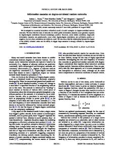
3. RESULTS We implemented all three algorithms from the last section including their modifications in C++ and a parallel version of the ”Go with the Winners” using the Message Passing Interface(MPI). The sequential algorithms have been run on a linux workstation with one 1GHz Pentium processor and 256Mb RAM. The parallel version of ”Go with the Winners” have been run on a LAM/MPI [5, 24] cluster. We used the degree sequence from the network of transcriptional regulation in E.coli as input to test the algorithms (see Figure 3.1). Each vertex in it represents a gene. An edge between two vertices is drawn if there is experimental evidence that the source is a transcription factor that regulates the target gene. This information was collected from RegulonDB [21] and some additional literature by the authors of [22]. We used also some toy-size degree sequences, where we could calculate the cardinality of G in a brute force way. The comparison of running times using the degree sequence from the E.coli network is given in Table 3.1.
3.1 The Switching Algorithm The switching algorithm shows good performance, because it needs O(E) time to come to completion. Using inputs of small size we observed that τ = E is sufficient for good sampling. The authors of [15] performed a simulation with the network of transcriptional regulation in E.coli and monitored the concentration of feedforward loops while increasing τ . Their results show that it converges after around E steps to some value, that seems to be the average number for directed graphs with this degree sequence. Therefore, they are hypothesizing that τ = 100 ∗ E should be more than adequate in practice. We run our implementation with this setting, but did not analyze if the samples are drawn uniformly from G. The algorithm produces a sample of size 100 of simple directed graphs with the same degree sequence as the E.coli network in 7 seconds (see Table 3.1).
3. Results
Algorithm Switching Matching unmodified Matching modified
Go with the Winners
34
Parameters τ = 100 ∗ E -
Statistics Time:7 sec restarts:29000 time:2h 24min 50sec ε = 1000 restarts:0.3 retries:11.9 time:6 sec B = 100 restarts:0 processors = 20 cloning steps:17.3 sync steps = 10 time:1min 48sec B = 100 restarts:0 processors = 2 cloning steps:14.7 sync steps = 10 time:7min 53sec
Tab. 3.1: Comparison of the running times using the degree sequence from the network of transcriptional regulation in E.coli as input. Each run generated 100 random directed graphs. restarts is the number of times that an algorithm discarded a partial configuration and started again from scratch. retries is the number of times that the modified version of the matching algorithm tried to correct an attempt to create a self- or a multiple edge. cloning steps is the number of cloning events during the Go with the Winners algorithm. These three values are averaged over the whole sample. processors is the number of processors used for the parallel version of Go with the Winners. sync steps is the rate at which the worker processes were synchronized.
3. Results
80
E.coli indegrees
70
35
6
E.coli outdegrees
5
60 4
50 40
3
30
2
20 1
10 0
0 0
50 100 150 200 250 300 350 400
0
50 100 150 200 250 300 350 400
Fig. 3.1: Statistics on the network of transcriptional regulation in E.coli. The X-axis denotes the labels of the vertices if sorted by indegree(left) or outdegree(right) in descending order. The Y-axis denotes the in- or the outdegree respectively. The graph contains 418 vertices and 519 edges with average of 1.2 edges per node. The maximum indegree is 72 and the maximum outdegree - 6.
3.2 The Matching Algorithm The unmodified version of the matching algorithm is as expected the slowest algorithm from all. Again, it performs relatively good on toy-size inputs, but using it to generate samples for background models for real data (such as the E.coli network) would clearly take more time that one can afford (see Table 3.1). The modified version of the matching algorithm runs in contrast much faster. Nevertheless, it is hard to estimate analytically how biased the generated samples are. Therefore, we analyzed them empirically. Although the 5 and discrepancy between Pa and Pb in the example of Figure 2.7 is only 432 does not seem to be significant, there are cases where the bias is considerably more tangible. If we let ε = 1000 and take the following degree sequenceh(0, 10), (1, 1), (1, 1), (1, 1), (1, 1), (1, 1), (1, 1), (1, 1), (1, 1), (1, 1), (1, 1), (10, 0)i and its realizations (Figure 3.2), we will see that the digraph in Figure 3.2a) is drastically undersampled. This degree sequence is derived from the previous example by multiplying the number of internal nodes (2-10 in Figure 3.2). In this way node 1 becomes an outgoing hub and node 12 an incoming hub. There are two distinct topologies - both hubs are connected to all of the internal nodes (Figure 3.2a) or there is one edge between two internal nodes (Figure 3.2b). There are 90 possible digraphs from the second type and
3. Results
a) 1 configuration
1
36
b) 90 configurations
2
2
3
3
4
4
5
5
6
12
1
6
7
7
8
8
9
9
10
10
11
11
12
Fig. 3.2: Example of biased sampling of the modified version of the matching algorithm
3. Results
37
ε Figure 3.2a Figure 3.2b Retries Mean Retries STD 0 1078 ∼ 1100 ∼ 2000 ∼ 2000 1 516 ∼ 1100 ∼ 650 ∼ 650 2 289 ∼ 1100 ∼ 320 ∼ 320 1000 53 ∼ 1100 ∼ 67 ∼ 67 Tab. 3.2: Statistics for the generation process of the 91 different graphs from Figure 3.2 with Algorithm 2.2.3. The counts for Figure 3.2b) are averaged over all 90 configurations. The mean and the standard deviation of the number of retries are averaged over all 91 configurations.
because they are all isomorph, their probabilities will be equal even with the modified version of the matching algorithm. To calculate them and the probability of Figure 3.2a) exactly will be very time and space consuming due to the combinatorial complexity. Therefore, we examined empirically their frequencies in a sample of 100000 runs of Algorithm 2.2.3. The digraph of Figure 3.2a) was generated 53 times, where each of the other 90 was generated 1100 times on average. We measured the number of times that both topologies were generated on average for different values of ε, the mean number of retries and its standard deviation (Table 3.2). The number of retries does not differ significantly if the final result is a digraph of type Figure 3.2a) or Figure 3.2b) and is geometrically distributed with mean given in Equation 2.5 for ε = 0. For ε > 0 the mean number of retries decreases as expected, but is hard enough to calculate it analytically. Our results are confirmed also by the simulations performed in [15] and clearly show that the bias could become significant for specific degree sequences.
3.3 The ”Go with the Winners” Algorithm The parallel implementation of the ”Go with the Winners” algorithm distributes the particles evenly among the nodes of the cluster. Generally, the processes on the cluster are divided into a single coordinator process and multiple workers. Each worker receives a subset of configurations (called minicolony) that are computed sequentially then. If their number drops under the half of the initial size of the minicolony, then all of the remaining configurations are cloned until the size of the minicolony grows to a number that is more than the half of its initial value. Furthermore, it is still possible that a worker discards all of its configurations due to some attempts to create self- or multiple edges. In this case it sends a message to the coordinator and
3. Results
38
waits to be synchronized with another worker. The coordinator performs synchronization steps at a predefined constant rate (for example every 10 steps). It waits for all the workers to report their current progress and then decides upon the strategy of the load balancing. In our implementation we used a simple one. We divide the nodes into two categories: alive and dead, according to whether they have some configurations available at the current step or not. If there are more dead than alive nodes, we assign to each alive node a number of dead nodes and require from it to send them its whole minicolony. In this way one actually clones the whole worker process, but this still has the same effect. The parallel version of the ”Go with the Winners” runs also quite fast. A run on 20 nodes with B = 100 generates a single directed graph with the same degree sequence as the E.Coli network in around one second on average.
4. DISCUSSION The problem of random generation of graphs is far from exhausted with this work. Many questions remain open. For example, one could notice that the rigorous analysis of the time complexity of all three algorithms stops at the point where one needs to know the exact number of all possible directed graphs with this degree sequence. It is hard to say anything about the convergence rate of the Markov chain. The probability for the matching algorithm to come to completion is also hard to calculate and the number of particles that are needed at the beginning of the ”Go with the Winners” algorithm is undetermined for the same reason. Although there is a series of papers [1, 2, 11, 23] trying to resolve this issue, the best known result to our knowledge is an approximation for N that is true for a fixed upper bound on the in- and outdegrees and n → ∞. In our toy examples it did not predict even close to the actual number of digraphs. Therefore, it is hard to tell how good it may be if used in real situations. This brings our attention to the second problem: how many directed graphs does one have to generate in order to be confident when making a statistical statement? If the space G contains billions of billions representatives and the size of the sample generated by the algorithm is only some couple of thousands, it may be very well possible that one draws wrong conclusions about the significance of the quantities that are measured in the original data. One should think of some way to evaluate the robustness of the algorithms used for the background model. A third problem is how to estimate the bias of the modified version of the matching algorithm. It is clear that the more retries are allowed the more tangible it becomes. The authors of the mfinder software [15, 22] use this algorithm for the background model that assesses the statistical significance of the network motifs in various graphs and claim that the bias is acceptable, but in our opinion it needs more rigorous analysis. A similar problem occurs when one decides how to set the sample weights for the ”Go with the Winners” algorithm. It is not obvious why 2−c is a correct choice. According to the theory of importance sampling [4], in any sampling procedure where one makes a decision with probability p in order to obtain an unbiased sample, one could replace p with p0 and correct for
4. Discussion
40
this by setting the sample weight to pp0 . In our opinion it is not clear that in the case of generation of random graphs with the ”Go with the Winners” algorithm why pp0 = 2−c . We leave this issue as an open question. It is worth noting that parallel versions of ”Go with the Winners” algorithms exist already for some problems [18]. The structure of the parallel architecture also imposes some computational burden. For example, the nodes have to be synchronized from time to time via messages. To analyze rigorously this overhead is also tricky since it requires some knowledge about the topology of the decision tree of the matching algorithm. Thus, we leave it as an open question. Yet another problem that surely deserves attention is the one of generating isomorphic graphs. None of the algorithms described in this work deal with it. The problem is that the space G contains classes of isomorphic graphs and their number is hard to calculate since it depends on the cardinality of G. Even worse, if one knows this cardinality, to calculate the number and the sizes of the isomorphic classes requires the usage of the Polya’s Theory of Counting [19], which makes it quite complicated not only from the analytical but also from the practical side. Very often to evaluate a formula derived by this means takes more time than to enumerate all possibilities in a brute-force way and just do the counts. It is easily seen why isomorphic classes cause a problem. Depending on the degree sequence not all of them might be of size one. In fact, for degree sequences from real networks it is highly unlikely to be so. Thus, if one starts to sample from G without correcting for this, the results will be biased. To the best of our knowledge, no one in the field of network motifs discovery had payed attention to this problem. To conclude the discussion we should say that generating random directed graphs with the same degree sequence as the original network may not be always an appropriate null hypothesis. In many cases it is questionable if this property actually reflects the natural constraints that govern the world that has been modeled. One could think of alternative ways to describe the background distribution. For example, by generating random directed graphs that have a certain minimal or maximal path lengths, number of cycles, girth, concentrations of subgraphs, etc. It is very well possible that such requirements complicate the synthesis and analysis of the algorithms that sample from these spaces and therefore will be a good challenge from computer science point of view. Another approach would be to compile a finite set of production rules for directed graphs called ”graph grammar”. Then one could implement a probabilistic algorithm that generates words from the language defined by this grammar and analyze their properties. The crucial issue in this case is how to choose the production rules and their
4. Discussion
41
probabilities so that they reflect the phenomena from the field of interest. All of this and surely more challenging questions will be in our opinion subject of the future work in this area.
5. SUMMARY In this work we analyzed three algorithms for uniform generation of directed graphs with prescribed degree sequence: the switching, the matching and ”Go with the Winners” algorithms. Each of them has its advantages and drawbacks. The switching algorithm is correct in the limits and quite fast in practice because it runs in linear time and space, but one cannot tell if the output is drawn from the stationary distribution. The matching algorithm is correct also but comes to completion with very low probability for degree sequences derived from real data. Its modified version runs in contrast much faster but produces biased samples that are complicated to analyze. The ”Go with the Winners” algorithm samples also non-uniformly but it is possible to correct it by assigning appropriate weights to the output. Its parallel version runs also quite fast and is therefore a good alternative to the other two. To give a straightforward criterium which one to choose is hard and probably application-dependant. In our opinion, to make the right decision requires more evaluation and analysis in the future.
6. ACKNOWLEDGEMENTS First of all, I am very grateful to Prof. Martin Vingron for supervising my thesis. It was a pleasure to work with him and I have learnt many new things during this time. Furthermore, I would like to thank to Debora Marks from the Harvard Medical School for bringing our attention to the problem of network motif detection in the context of our work on micro-RNAs. I would like to thank to Dr. Behshad Behzadi for his critical review of this manuscript and for pointing and discussing with me a great deal of issues that stemmed from it. Also, I am very thankful to Dr. Clemens Gr¨opl for his help as a second reviewer of my thesis. I would like to thank to Dr. Stephan R¨opcke for discussing with me many of the problems during my work. I would like to thank to Todor Koev for reading the manuscript and improving the quality of the text and to Boyko Amarov for the endless nights he spent to talk with me about probabilities and statistics. I really appreciate their help. I would like to thank to all my friends and especially to my parents, Plamen and Tsvetanka Fizievi, for their continuous support along my study and this work in particular. Last but not least, I would like to thank to the Max Planck Institute for Molecular Genetics for the financial support that it would surely be much more difficult to complete my diploma thesis without.
BIBLIOGRAPHY [1] A.B´ ek´ essy, P.B´ ek´ essy, and J.Koml´ os. Asymptotic enumeration of regular matrices. Studia Scientiarum Mathematicarum Hungarica, 7:343– 353, 1972. [2] E.A. Bender. The asymptotic number of non-negative integer matrices with given row and column sums. Discrete Mathematics, 10:217–223, 1974. [3] B. Bollobas. Random Graphs. Cambridge University Press, 2001. [4] J.A. Bucklew. Introduction to Rare Event Simulation. Springer-Verlag, New York, 2004. [5] G. Burns, R. Daoud, and J. Vaigl. LAM: An Open Cluster Environment for MPI. Proceedings of Supercomputing Symposium, pages 379–386, 1994. [6] P. Erdos and A. Renyi. On Random Graphs I. Publ. Math. Debrecen, 6(290), 1959. [7] W. Feller. An Introduction to Probability Theory and its Applications. Wiley, New York, 1968. [8] S. Itzkovitz and U. Alon. Subgraphs and network motifs in geometric networks. Phys Rev E Stat Nonlin Soft Matter Phys, 71(2 Pt 2):026117, 2005. 1539-3755 Journal Article. [9] S. Itzkovitz, R. Milo, N. Kashtan, G. Ziv, and U. Alon. Subgraphs in random networks. Phys Rev E Stat Nonlin Soft Matter Phys, 68(2 Pt 2):026127, 2003. 1539-3755 Journal Article. [10] R. Kannan, P. Tetali, and S. Vempala. Simple Markov-Chain algorithms for generating bipartite graphs and tournaments. In Symposium on Discrete Algorithms, pages 193–2000, 1997.
Bibliography
45
[11] L. Katz and J.H. Powell. The number of locally restricted directed graphs. Proceedings of the American Mathematical Society, 5:621–626, 1954. [12] M. Krause. A Simple Proof of the Gale-Ryser Theorem. Amer. Math. Monthly, 103:335–337, 1996. [13] N. Metropolis and S. Ulam. The Monte Carlo Method. J. Amer. Stat. Assoc. 44, 335-341, 1949. [14] R. Milo, S. Itzkovitz, N. Kashtan, R. Levitt, S. Shen-Orr, I. Ayzenshtat, M. Sheffer, and U. Alon. Superfamilies of evolved and designed networks. Science, 303(5663):1538–42, 2004. 1095-9203 Journal Article. [15] R. Milo, N. Kashtan, S. Itzkovitz, M.E.J. Newman, and U. Alon. On the uniform generation of random graphs with prescribed degree sequences. arXiv:cond-mat/0312028, 2004. [16] R. Milo, S. Shen-Orr, S. Itzkovitz, N. Kashtan, D. Chklovskii, and U. Alon. Network motifs: simple building blocks of complex networks. Science, 298(5594):824–7, 2002. 1095-9203 Journal Article. [17] W. Nadler and P. Grassberger. ”Go with the Winners” simulations. preprint cond-mat/0010265, 2000. [18] M. Peinado and T. Lengauer. Parallel ”Go with the Winners Algorithms” in the LogP Model. IPPS: 11th International Parallel Processing Symposium, 1997. [19] G. Polya, R. Tarjan, and D. Woods. Notes on Introductory Combinatorics,Progress in Computer Science No. 4. Birkhauser, Boston, Basel, Stuttgart, 1983. [20] A.R. Rao, R. Jana, and S. Bandyopadhyay. A Markov Chain Monte Carlo Method for Generating Random (0,1)-Matrices. The Indian Journal of Statistics, 58:225–242, 1996. [21] H. Salgado, A. Santos-Zavaleta, S. Gama-Castro, D. Millan-Zarate, E. Diaz-Peredo, F. Sanchez-Solano, E. Perez-Rueda, C. BonavidesMartinez, and Collado-Vides J. RegulonDB (version 3.2): transcriptional regulation and operon organization in Escherichia coli K-12. Nucleic Acids Res., 29(1):72–74, 2001.
Bibliography
46
[22] S. S. Shen-Orr, R. Milo, S. Mangan, and U. Alon. Network motifs in the transcriptional regulation network of Escherichia coli. Nat Genet, 31(1):64–8, 2002. 1061-4036 Journal Article. [23] T. Snijders. Enumeration and simulation methods for 0-1 matrices with given marginals. Psychometrika, 56:397–417, 1991. [24] J.M. Squyres and A. Lumsdaine. A Component Architecture for LAM/MPI. Proceedings, 10th European PVM/MPI Users’ Group Meeting, 2840:379–387, September / October 2003. [25] R. Taylor. Constrained switchings in graphs. Lecture Notes in Mathematics, 884:314–336, 1981. [26] U.V. Vazirani and D. Aldous. ”Go With the Winners” Algorithm. Proceedings of the IEEE Symposium on Foundations of Computer Science, pages pp. 492–501, 1994. [27] F. Viger and M. Latapy. Fast generation of random connected graphs with prescribed degrees. arXiv:cs.NI/0502085, 2005.