AIAA 2014-0299 AIAA SciTech 13-17 January 2014, National Harbor, Maryland 16th AIAA Non-Deterministic Approaches Conference
Uncertainty Propagation with Monotonicity Preserving Robustness Jeroen A.S. Witteveen∗ Center for Mathematics and Computer Science (CWI), Science Park 123, 1098XG Amsterdam, The Netherlands
Downloaded by Jeroen Witteveen on January 28, 2014 | http://arc.aiaa.org | DOI: 10.2514/6.2014-0299
Gianluca Iaccarino† Mechanical Engineering, Stanford University, Building 500, Stanford, CA 94305-3035, USA Uncertainty progagation is a non-deterministic approach that is essential in a validation process to increase the confidence in the numerical predictions by quantifying the uncertainties. These uncertainty quantification methods need to be at least as robust as the spatial discretization method to actually improve the reliability of the simulation results. A number of advanced robustness criteria have been well-established in Finite Volume Methods (FVM) such the Local Extremum Diminishing (LED) concept and the Monotonicity Preserving (MP) principle. However, it has been shown that LED methods are limited to at most first-order accuracy for non-monotonic solutions. Therefore, the MP concept is here introduced into a non-deterministic method to obtain a robust and higher-order quantification of uncertainties. Two formulations of the MP limiter that will be considered for a sinusoidal test function, a random wave equation, and a transonic RAE2822 airfoil flow reveal that non-monotonic responses can lead to lower sensitivities.
I.
Introduction
The need for accurate resolution of shock waves in Computational Fluid Dynamics (CFD) is a major driver in the development of robust numerical methods for approximating discontinuities. The Local Extremum Diminishing (LED) robustness concept has, for example, been introduced into the Finite Volume Method (FVM) for preventing overshoots at discontinuities.9 However, LED schemes have the disadvantage that they reduce to first-order accuracy at physical local extrema in the solution.10 Monotonicity-Preserving (MP) limiters have therefore been developed which do not affect the accuracy at smooth extrema.4 A straightforward approach to avoid the clipping of extrema is to turn off the convexity-preserving constraints in cells with a non-monotonic solution.11 These cells can be identified by a change in the sign of the discrete derivatives over the volume, in combination with a tolerance for distinguishing physical extrema from spurious numerical oscillations. Because of the dependence on this threshold value, it can be difficult to differentiate between smooth and non-smooth extrema. Therefore, a second MP approach has been proposed which automatically enlarges the limiter intervals near physical extrema in such a way that the solution is continuously dependent on the data.16 See Figure 1 for sketches of these LEC and MP limiters for FVM in the physical space. The robust approximation of discontinuities is also important in Uncertainty Quantification (UQ), since nonlinearities can result in strong amplification of input uncertainties during their propagation through a computational model. In that respect, the introduction of FVM robustness concepts into multi-element UQ methods seems promising, because their local tessellation of the probability space into multiple subdomains is comparable to spatial FVM discretizations in physical space. These multi-element methods3, 6, 12 usually ∗ Scientific † Associate
Staff Member, AIAA Member, Phone: +31(0)20 592 4085, Fax: +31(0)20 203 1226,
[email protected]. Professor, AIAA Member,
[email protected].
1 of 11 American Institute of Aeronautics and Astronautics Copyright © 2014 by J.A.S. Witteveen, G. Iaccarino. Published by the American Institute of Aeronautics and Astronautics, Inc., with permission.
(a) LEC limiter
(b) MP limiter11
(c) MP limiter16
Downloaded by Jeroen Witteveen on January 28, 2014 | http://arc.aiaa.org | DOI: 10.2514/6.2014-0299
Figure 1. Limiters in the FVM discretization of the physical space.
employ global UQ methods7, 22 confined to hypercube subdomains. FVM approaches have been used in UQ in the form of the Essentially Non-Oscillatory (ENO) scheme,1, 2, 5, 19 upwind discretizations,17 and subcell resolution.18 Global UQ methods for approximating stochastic discontinuities are, for example, based on entropic variables14 and iterative formulations.15 The LED concept has also been extended successfully to UQ in terms of the Local Extremum Conserving (LEC) limiter for interpolation in the Simplex Stochastic Collocation (SSC) method20, 21 to avoid overshoots in the approximation of discontinuous response surfaces. However, it has been observed that the LEC limiter leads to a linear first-order approximation at local extrema in the probability space as well. The MP concept is here introduced into UQ to achieve higher-order approximations of local minima and maxima in the SSC method, while at the same time improving robustness at discontinuities. Formulation of the MP limiter in probability space is developed in the context of the SSC framework in Section II. The properties of the resulting SSC–MP method are demonstrated for a sinusoidal test function in Section III. In Sections IV and V, the application to a random wave equation and the transonic flow over the RAE2822 airfoil is considered. Conclusions and opportunities for future work are summarized in Section VI.
II.
Simplex stochastic collocation with monotonicity-preserving limiter
The SSC method is based on a simplex elements tessellation of the probability space and higher-degree polynomial interpolation of samples at the vertexes of the simplexes, as described in Section II.A. The LEC limiter for the interpolant is briefly reviewed in Section II.B and the MP limiter is introduced in Section II.C. II.A.
The simplex stochastic collocation framework
The SSC approach20, 21 calculates the probability distribution of an output quantity of interest u(x, ξ) for a computational problem subject to a vector of nξ second-order random parameters ξ = {ξ1 , . . . , ξnξ } ∈ Ξ in the initial and boundary conditions or in the mathematical model. The probability density fξ (ξ) of the random parameters ξ in the parameter space Ξ ⊂ Rnξ is assumed to be known. This parameter space Ξ is discretized by Snethe SSC method using a Delaunay tessellation of ne non-overlapping simplexes Ξj , for which holds Ξ = j=1 Ξj . Computationally intensive deterministic solutions vk (x) = u(x, ξ k ) of the governing equations are calculated for the parameter values that correspond to the ns sampling points ξ k at the vertexes of the simplexes Ξj . The initial sampling points ξ k are given by deterministic sampling at the corners of the parameter space Ξ and at the nominal conditions. Additional sampling points are subsequently determined based on random sampling in the simplexes Ξj with the highest values of a solution-based refinement measure that depends on the local polynomial degree pj , which results in the set of samples v(x) = {v1 (x), . . . , vns (x)}. The response surface for u(x, ξ) in Ξ is approximated by a higher-degree piecewise polynomial interpolation w(x, ξ) of the samples v(x). The approximation w(x, ξ) is constructed using a polynomial chaos expansion7
2 of 11 American Institute of Aeronautics and Astronautics
in each of the simplexes Ξj in terms of the basis polynomials Ψj,i (ξ) Pj (x)
wj (x, ξ) =
X
cj,i (x)Ψj,i (ξ),
(1)
i=0
with w(x, ξ) = wj (x, ξ) for ξ ∈ Ξj and Pj (x) + 1 = (nξ + pj (x))!/(nξ !pj (x)!) the number of expansion terms, where pj (x) is the local polynomial degree of wj (x, ξ) in Ξj . The coefficients cj,i (x) are determined by interpolating the samples vk (x) of a stencil Sj (x) = {ξ kj,0 , . . . , ξ kj,N (x) } of Nj (x) + 1 unique sampling j points ξ k , with kj,l ∈ {1, . . . , ns } and l = 0, . . . , Nj (x). The higher-degree stencils Sj (x) consist of the nξ + 1 sampling points ξ k at the vertexes of the simplex Ξj and Nj (x) − nξ other sampling points at the vertexes of surrounding simplexes. The statistical moments of u(x, ξ) are finally approximated by integrating w(x, ξ) over the parameter space Ξ using a Monte Carlo evaluation with nmc ≫ ns integration points ξ mck .
Downloaded by Jeroen Witteveen on January 28, 2014 | http://arc.aiaa.org | DOI: 10.2514/6.2014-0299
II.B.
Local extremum conserving limiter
The higher-degree interpolation w(x, ξ) obtains an accurate approximation of smooth monotonic response surfaces u(x, ξ). In order to also ensure a robust interpolation at discontinuities in the probability space, the LEC limiter eliminates overshoots and undershoots of the interpolation w(x, ξ) with respect to the samples v. It reduces locally the size of the stencil Sj (x) and the polynomial degree pj (x) of Ξj by one until the following LEC condition is satisfied20 min wi (x, ξ) = min vi (x) ∧ max wi (x, ξ) = max vi (x), ξ∈Ξi
ξ∈Ξi
(2)
in all simplexes Ξi that are contained in the stencil Sj (x) of the simplex Ξj , with vi (x) = {vki,0 (x), . . . , vki,nξ (x)} the samples vk (x) at the vertexes ξ k of the simplex Ξi . The interpolation w(x, ξ) is then LED with respect to the response u(x, ξ), since the samples v are LED with respect to u(x, ξ) for vk (x) = u(x, ξ k ). The limiter automatically reduces the polynomial degree pj (x) to a piecewise linear interpolation at discontinuities, which always satisfies Eq. (2). However, it can also limit the polynomial degree to pj (x) = 1 at local extrema in the response surface, which results in an undesirable first-order approximation of smooth non-monotonic solutions. II.C.
Monotonicity-preserving limiter
The MP limiter combines the monotonicity of the approximation at discontinuities with higher-degree interpolation at smooth local extrema through a three-step implementation. The first step is the replacement of the LEC condition Eq. (2) with an MP condition in the interior of the simplexes Ξj , since Eq. (2) does not necessarily result in a monotonic interpolation in Ξj as long as no artificial extrema exceed the sampled values vj . This requirement is enforced by making a Delaunay sub-tessellation in Ξj of the vertexes ξ k of Ξj and the Monte Carlo (MC) points ξ mck in Ξj for integrating w(x, ξ). If the value w(x, ξ mck ) at any of the MC points ξ mck of this simplex sub-triangulation in Ξj is larger or smaller than the value at all other vertexes of all sub-simplexes of which ξ mck is a vertex, then the interpolation wj (x, ξ) is non-monotonic. The polynomial degree pj (x) and the stencil Sj (x) of Ξj are then reduced similarly as for the LEC limiter. This MP criterion is more restrictive than that of the LEC version, and it is always satisfied for a reduction to pj (x) = 1. The second part is to turn off the MP limiter at local extrema in the solution, since at these locations there is no monotonicity in the response that can be preserved. This is the stochastic equivalent of the MP limiter for FVM in the physical space by11 in the sense that it deactivates the limiter at local extrema. These extrema in u(x, ξ) are identified by local extrema in the samples v in the interior of Ξ, since u(x, ξ) has a local extremum if vk (x) is also a local extremum. A local extremum at ξ k is again detected if vk (x) is larger or smaller than the samples in all other vertexes of all simplexes that contain ξ k . If vk (x) is such a local extremum, then the MP limiter is deactivated in all simplexes of which ξ k is a vertex. In order to avoid overshoots, it is important to turn the MP limiter off only at smooth extrema in the solution and not for extrema at discontinuities. The gradient magnitude of a linear interpolation in Ξj is used in the third step to detect the latter non-smooth extrema. If the gradient in any of the simplexes that contain the local extremum ξ k surpasses a threshold value, then ξ k is not treated as a smooth extremum and the MP limiter is retained in all simplexes that contain the vertex ξ k . The second formulation of the 3 of 11 American Institute of Aeronautics and Astronautics
MP limiter in FVM by16 based on enlarging the limiter intervals will be extended in future work, since it is expected to give equally robust results without the sensitivity to a threshold parameter.
III.
A sinusoidal test function
The SSC method is first applied to the following non-monotonic sine function (3)
in order to quantify the impact of the MP limiter on the approximation of smooth extrema. The constant c = 2.5 ensures that the function has a local maximum in the range of the uniformly distributed random parameter ξ = U (0, 1), as can be seen in Figure 2. Figure 2(a) and (b) shows the SSC results based on the LEC and MP limiters with ns = 5 samples compared to a MC reference solution with nmc = 50, 000 samples. Since the LEC limiter does not allow overshoots in the interpolation w(ξ) with respect to the samples v, the robustness of the LEC limiter for the approximation of discontinuities also reduces the interpolation to a piecewise linear function around the local maximum. This leads to a relatively large approximation error at the local extremum. In contrast, the MP limiter detects the local maximum in the solution in the form of the local maximum in the samples at ξ = 0.75. The MP constraint is therefore turned off in the elements to the left and the right of ξ = 0.75. This results in a suitable global fourth-order polynomial approximation of the smooth response with a local maximum beyond the samples, which accurately approximates the reference solution. 1.1 1
1.1
LEC samples MC
1 0.9
0.8
0.8
0.7
0.7
0.6
0.6
MP samples MC
u
0.9
u
Downloaded by Jeroen Witteveen on January 28, 2014 | http://arc.aiaa.org | DOI: 10.2514/6.2014-0299
u(ξ) = sin(cξ),
0.5
0.5
0.4
0.4
0.3
0.3
0.2
0.2
0.1
0.1
0 0
0.1
0.2
0.3
0.4
0.5 ξ
0.6
0.7
0.8
0.9
0 0
1
0.1
0.2
0.3
(a) LEC limiter
0.4
0.5 ξ
0.6
0.7
0.8
0.9
1
(b) MP limiter
Figure 2. Response surface approximation for the sine function with ns = 5.
The effect of the different response surface approximations on the convergence of the RMS error with respect to the MC reference solution is shown in Figure 3 as a function of the number of samples ns . The LEC limiter results in a slow first-order error convergence due to the piecewise linear approximation at the maximum. Superlinear convergence to machine precision is obtained by the higher-degree approximation of the MP limiter owing to the simultaneous increase of the polynomial degree with the number of samples. This leads to the reduction of the RMS error by many orders of magnitude. In Figure 3(b) the local error in the LEC approximation is displayed for ns = 17. This result illustrates that the error in the LEC solution is dominated by the piecewise linear approximation of the local maximum around ξ = 0.628. The convergence for the statistical moments in terms of the mean µu and the standard deviation σu is given in Table 1 as a function of ns for the LEC and MP limiters compared to the MC reference solution. For the MP limiter the statistics converge to the MC results for ns = 9. The LEC limiter leads to larger initial errors for ns = 3 and does not reach the MC solution for ns = 17. It also consistently underpredicts the mean and the standard deviation for this concave function.
IV.
Random wave equation
The characteristics of the MP limiter in a problem that combines a discontinuity with local extrema in the response are demonstrated for a random wave equation. The following linear wave equation for u(x, t, ξ) 4 of 11 American Institute of Aeronautics and Astronautics
−3
0
10
3.5
LEC MP
x 10
3 2.5
−5
10
error
error
2 1.5 −10
10
1 0.5 −15
10
0
1
10
0 0
2
10 samples
10
(a) RMS error convergence.
0.1
0.2
0.3
0.4
0.5 ξ
0.6
0.7
0.8
0.9
1
(b) Local error by the LEC limiter with ns = 17
Downloaded by Jeroen Witteveen on January 28, 2014 | http://arc.aiaa.org | DOI: 10.2514/6.2014-0299
Figure 3. Error in the response surface approximation for the sine function.
Table 1. Convergence of µu and σu by the LEC and MP limiters compared to the MC reference solution for the sine function.
ns 3 5 9 17 MC
µu LEC MP −1 6.2410 · 10 7.3239 · 10−1 7.0606 · 10−1 7.2034 · 10−1 7.1844 · 10−1 7.2045 · 10−1 7.2020 · 10−1 7.2045 · 10−1 7.2045 · 10−1
σu LEC MP −1 2.5501 · 10 2.5957 · 10−1 2.6355 · 10−1 2.7751 · 10−1 2.7523 · 10−1 2.7720 · 10−1 2.7695 · 10−1 2.7720 · 10−1 2.7720 · 10−1
has been proposed by8
∂u ∂u − a(ξ) = 0, (4) ∂t ∂x on the spatial domain x ∈ [−1, 1]. The random wave speed a(ξ) = cξ changes sign with ξ = U (−1, 1) and a constant c = 0.5. The time-dependent inflow boundary conditions are defined as u(−1, t, ξ) = sin(2π(a(ξ)t − 1)),
ξ < 0,
(5)
u(1, t, ξ) = sin(π(a(ξ)t + 1)),
ξ ≥ 0,
(6) (7)
with compatible initial conditions u(x, 0, ξ) =
(
sin(2πx), sin(πx),
The analytical solution of (4) to (8) is given by ( sin[2π(a(ξ)t + x)], u(x, t, ξ) = sin[π(a(ξ)t + x)],
ξ < 0, ξ ≥ 0.
ξ < 0, ξ ≥ 0,
(8)
(9)
which results in smooth non-monotonic realizations as a function of x in the physical space on both sides of a discontinuity in the parameter space at ξ = 0. Knowledge about the discontinuity location is not used in solving the problem, since in general it might not be available. The solution is first considered at one spatial location, x = 0.55, for t = 1 with adaptive refinement to ns = 25. The response surface approximations resulting from the LEC and MP limiters are compared to an MC reference solution with nmc = 50, 000 in Figure 4. The figure shows a challenging response surface with a smooth local maximum at ξ = −0.6 and two other extrema at the left and the right of a discontinuity. 5 of 11 American Institute of Aeronautics and Astronautics
The LEC limiter leads to equal refinement at both the discontinuity and the smooth local maximum in Figure 4(a), because the refinement measure depends on the local polynomial degree that is also reduced to a piecewise linear function at the smooth extremum. This gives a less sharp resolution of the discontinuity compared to the MP limiter in Figure 4(b). The MP limiter only refines the samples at the step since it results in a higher-degree approximation of the smooth maximum. The jump is robustly approximated with a piecewise linear interpolation, because the MP limiter is not turned off in the elements that contain a local extremum at a discontinuity such that overshoots of the samples are avoided. The discontinuity is detected in terms of a threshold for the gradient magnitude for which the value of 5 is used in this case. The error in µu and σu for the discretization with ns = 25 is given in Table 2, and the RMS error convergence is shown in Figure 5 up to ns = 50. The faster convergence of the MP limiter results in errors an order of magnitude lower than those of the LEC limiter, mainly because of the sharper resolution of the discontinuity. 1.2
0.8
0.8
0.6
0.6
0.4
0.4
0.2
0.2
0
0
−0.2
−0.2
−0.4 −1
−0.8
−0.6
−0.4
−0.2
0 ξ
0.2
0.4
0.6
0.8
MP samples MC
1
u
u
1
−0.4 −1
1
−0.8
−0.6
(a) LEC limiter
−0.4
−0.2
0 ξ
0.2
0.4
0.6
0.8
1
(b) MP limiter
Figure 4. Response surface approximation for the random wave equation at x = 0.55 with adaptive refinement to ns = 25.
Table 2. Error in µu and σu by the LEC and MP limiters with respect to the MC reference solution for the random wave equation at x = 0.55 with adaptive refinement to ns = 25.
MC mean µu st.dev. σu
error ε −1
5.6733 · 10 3.5910 · 10−1
LEC 1.0114 · 10−2 1.1978 · 10−2
MP 1.2535 · 10−3 1.5498 · 10−3
0
10
LEC MP
−1
10
error
Downloaded by Jeroen Witteveen on January 28, 2014 | http://arc.aiaa.org | DOI: 10.2514/6.2014-0299
1.2
LEC samples MC
−2
10
−3
10
0
10
1
10 samples
2
10
Figure 5. RMS error convergence by the MP limiter for the random wave equation at x = 0.55 with adaptive refinement to ns = 50.
The convergence of µu (x) and σu (x) over the entire spatial domain x ∈ [−1, 1] is shown in Figures 6 and 7 for ns = {20, 30}. The adaptive refinement measure is here based on the minimum of the local polynomial degree pj in an element Ξj over all nx = 100 spatial points. The statistics show a smooth
6 of 11 American Institute of Aeronautics and Astronautics
oscillatory behavior as a function of x, just like each of the samples. The MP limiter gives a more accurate approximation of the MC reference solution than the LEC limiter, especially for σu (x). The underlying response surface approximations for u(x, 1, ξ) over the physical coordinate x and the stochastic dimension ξ are given in Figure 8. The figure shows two oscillating responses with different wave numbers at both sides of the discontinuity at ξ = 0, which has a varying strength as a function of x. The black lines at constant ξ-values denote the sampling locations that follow from the LEC and MP limiters. The LEC limiter results in almost uniform refinement, since it also adapts to the location of the local extrema, which move in ξ as a function of x. This does not affect the sampling of the MP limiter, which focuses on resolving the discontinuity. Therefore, the MP limiter shows the most improvement in the approximation of the standard deviation with respect to the LEC limiter in Figure 7 at x-locations where the jump at the discontinuity location is the largest. 0.8
0.4
0.4
0.2
0.2
0
0
−0.2
−0.2
−0.4
−0.4
−0.6
−0.6
−0.8 −1
−0.8
−0.6
−0.4
−0.2
0 x
0.2
0.4
0.6
0.8
20 25 30 MC
0.6
mean u
mean u
0.6
−0.8 −1
1
−0.8
−0.6
−0.4
(a) LEC limiter
−0.2
0 x
0.2
0.4
0.6
0.8
1
(b) MP limiter
Figure 6. Mean µu (x) for the random wave equation with adaptive refinement.
0.9
0.9
20 25 30 MC
0.8
20 25 30 MC
0.8 0.7
0.6
0.6
std u
0.7
std u
Downloaded by Jeroen Witteveen on January 28, 2014 | http://arc.aiaa.org | DOI: 10.2514/6.2014-0299
0.8
20 25 30 MC
0.5
0.5
0.4
0.4
0.3
0.3
0.2 −1
−0.8
−0.6
−0.4
−0.2
0 x
0.2
0.4
0.6
0.8
0.2 −1
1
−0.8
−0.6
(a) LEC limiter
−0.4
−0.2
0 x
0.2
0.4
0.6
0.8
1
(b) MP limiter
Figure 7. Standard deviation σu (x) for the random wave equation with adaptive refinement.
V.
RAE 2822 airfoil
The lift coefficient Cl has a non-monotonic dependence on the Mach number M in the standard transonic flow problem around the RAE 2822 airfoil.13 The uniform distribution for M is in that case defined by a mean of µM = 0.734 and standard deviation of σM = 0.005 at an angle of attack of α = 2.79o and a Reynolds number of Re = 6.5 · 106 . The fully turbulent flow problem is solved using the Fluent Reynoldsaveraged Navier-Stokes solver with the Spalart-Allmaras turbulence model and a second-order Roe upwind discretization on a two-dimensional mesh of 7.5 · 104 spatial cells, as shown in Figure 9. The height of the first cell layer above the airfoil is with 1 · 10−5 c smaller than the y + -value of 1 and the dimensions of the
7 of 11 American Institute of Aeronautics and Astronautics
Downloaded by Jeroen Witteveen on January 28, 2014 | http://arc.aiaa.org | DOI: 10.2514/6.2014-0299
(a) LEC limiter
(b) MP limiter Figure 8. Response surface approximation for the random wave equation with adaptive refinement to ns = 30.
8 of 11 American Institute of Aeronautics and Astronautics
(a) Mesh
(b) Zoom on the airfoil
Figure 9. Spatial computational mesh for the transonic flow over the RAE 2822 airfoil.
Approximation of the non-monotonic response surface of Cl as a function of M is shown in Figure 10 for the initial discretization of the LEC and MP limiters with ns = 3. The quadratic interpolation through the samples for the MP limiter already leads to a more realistic representation of the dependence of Cl on M . The LEC limiter gives a piecewise linear approximation because the sampling point at the nominal condition M = 0.734 is not exactly located at the maximum of Cl . This results initially for ns = 3 in an underprediction of the mean lift coefficient µCl for the LEC limiter, as demonstrated by the convergence in Table 3. The mean and standard deviation of the drag and pitching moment coefficients, Cd and Cm , respectively, are given in Table 4 for the MP limiter with ns = 9. Both Cd and Cm depend monotonically on M such that the LEC results are identical. The drag coefficient Cd has the highest coefficient of variation with CoVCd = 14.9%, and Cl is relatively the least sensitive to variations in M with CoVCl = 0.204% because of the non-monotonicity of its response surface. 0.795
l
0.7925
C
Downloaded by Jeroen Witteveen on January 28, 2014 | http://arc.aiaa.org | DOI: 10.2514/6.2014-0299
mesh are 32.5c × 25c, where c = 1 is the airfoil chord. Only the pressure forces on the airfoil are taken into account in computing Cl .
0.79
0.7875
0.785 0.7253
0.73
M
0.735
0.74
0.7427
Figure 10. Response surface approximation of Cl as a function of M by the LEC and MP limiters for the transonic flow over the RAE 2822 airfoil with ns = 3.
VI.
Conclusions
The LEC limiter in the SSC method for the robust approximation of discontinuities in the probability space also reduces the polynomial interpolation degree to a piecewise linear function at smooth local extrema in the response surface. Therefore, the MP limiter is introduced into UQ to combine a higher-degree
9 of 11 American Institute of Aeronautics and Astronautics
Table 3. Convergence of µCl by the LEC and MP limiters for the transonic flow over the RAE 2822 airfoil.
ns 3 5 9
LEC 7.9059 · 10−1 7.9117 · 10−1 7.9131 · 10−1
MP 7.9153 · 10−1 7.9115 · 10−1 7.9139 · 10−1
Table 4. Mean µ, standard deviation σ, and coefficient of variation CoV of the lift, drag, and pitching moment coefficients by the MP limiter for the transonic flow over the RAE 2822 airfoil with ns = 9.
Downloaded by Jeroen Witteveen on January 28, 2014 | http://arc.aiaa.org | DOI: 10.2514/6.2014-0299
Cl Cd Cm
µ 7.9139 · 10−1 1.4710 · 10−2 9.8398 · 10−2
σ 1.6140 · 10−3 2.1910 · 10−3 3.4812 · 10−3
CoV 2.0395 · 10−3 1.4895 · 10−1 3.5379 · 10−2
approximation of smooth non-monotonic solutions with a non-oscillatory interpolation at discontinuities. The approach deactivates the stricter MP limiter in elements that contain a local extremum, except at discontinuities. The MP limiter shows superlinear convergence to machine precision for a non-monotonic sinusoidal function compared to first-order convergence by the LEC limiter. In the application to a random wave equation with local extrema and discontinuities in the response surface, the MP limiter is an order of magnitude more accurate than the LEC limiter because it focuses on refining the discontinuity owing to the higher-degree approximation of the extrema. The MP limiter enables us to accurately resolve the non-monotonic response of the lift coefficient Cl as a function of the random Mach number for the RAE2822 transonic airfoil. This reveals that Cl is less sensitive to the uncertainty owing to the non-monotonicity of the response surface compared to the drag and moment coefficients Cd and Cm with monotonic responses. In the full paper, a second version of the MP limiter will be implemented that does not depend on a threshold value to distinguish between smooth and non-smooth extrema.
References 1 R. Abgrall, P.M. Congedo, A semi-intrusive deterministic approach to uncertainty quantification in non-linear fluid flow problems, Journal of Computational Physics 235 (2013) 828–845. 2 R. Abgrall, A simple, flexible and generic deterministic approach to uncertainty quantifications in nonlinear problems: application to fluid flow problems, 5th European Conference on Computational Fluid Dynamics, ECCOMAS CFD, Lisbon, Portugal (2010). 3 I. Babuˇ ska, R. Tempone, G.E. Zouraris, Galerkin finite elements approximation of stochastic finite elements, SIAM Journal on Numerical Analysis 42 (2004) 800–825. 4 D.S. Balsara, C.W. Shu, Monotonicity preserving weighted essentially non-oscillatory schemes with increasingly high order of accuracy, Journal of Computational Physics 160 (2000) 405–452. 5 T. Barth, On the propagation of statistical model parameter uncertainty in CFD calculations, Theoretical and Computational Fluid Dynamics 26 (2012) 435–457. 6 J. Foo, X. Wan, G.E. Karniadakis, The multi-element probabilistic collocation method (ME-PCM): error analysis and applications, Journal of Computational Physics 227 (2008) 9572–9595. 7 R.G. Ghanem, P.D. Spanos, Stochastic Finite Elements: A Spectral Approach, New York: Springer-Verlag (1991). 8 D. Gottlieb, D. Xiu, Galerkin method for wave equations with uncertain coefficients, Communications in Computational Physics 3 (2008) 505–518. 9 A. Jameson, Computational algorithms for aerodynamic analysis and design, Applied Numerical Mathematics 13 (1993) 383–422. 10 A. Jameson, Analysis and design of numerical schemes for gas dynamics, 1: Artificial diffusion, upwind biasing, limiters and their effect on accuracy and multigrid convergence, International Journal of Computational Fluid Dynamics 4 (1995) 171–218. 11 B.P. Leonard, A.P. Lock, M.K. Macvean, The NIRVANA scheme applied to one-dimensional advection, International Journal of Numerical Methods for Heat and Fluid Flow 5 (1995) 341–377. 12 O.P. Le Maˆ ıtre, H.N. Najm, R.G. Ghanem, O.M. Knio, Multi-resolution analysis of Wiener-type uncertainty propagation schemes, Journal of Computational Physics 197 (2004) 502–531. 13 G. Onorato, G.J.A. Loeven, G. Ghorbaniasl, H. Bijl, C. Lacor, Comparison of intrusive and non-intrusive polynomial chaos methods for CFD applications in aeronautics, 5th European Conference on Computational Fluid Dynamics, ECCOMAS CFD, Lisbon, Portugal (2010). 14 G. Po¨ ette, B. Despr´ es, D. Lucor, Uncertainty quantification for systems of conservation laws, Journal of Computational Physics 228 (2009) 2443–2467.
10 of 11 American Institute of Aeronautics and Astronautics
Downloaded by Jeroen Witteveen on January 28, 2014 | http://arc.aiaa.org | DOI: 10.2514/6.2014-0299
15 G. Po¨ ette, D. Lucor, Non intrusive iterative stochastic spectral representation with application to compressible gas dynamics, Journal of Computational Physics 231 (2012) 3587–3609. 16 A. Suresh, H.T. Huynh, Accurate monotonicity-preserving schemes with Runge-Kutta time stepping, Journal of Computational Physics 136 (1997) 83–99. 17 J. Tryoen, O. Le Maˆ ıtre, M. Ndjinga, A. Ern, Intrusive Galerkin methods with upwinding for uncertain nonlinear hyperbolic systems, Journal of Computational Physics 229 (2010) 6485–6511. 18 J.A.S. Witteveen, G. Iaccarino, Subcell resolution in simplex stochastic collocation for spatial discontinuities, Journal of Computational Physics 251 (2013) 17–52. 19 J.A.S. Witteveen, G. Iaccarino, Simplex stochastic collocation with ENO-type stencil selection for robust uncertainty quantification, Journal of Computational Physics 239 (2013) 1–21. 20 J.A.S. Witteveen, G. Iaccarino, Refinement criteria for simplex stochastic collocation with local extremum diminishing robustness, SIAM Journal on Scientific Computing 34 (2012) A1522–A1543. 21 J.A.S. Witteveen, G. Iaccarino, Simplex stochastic collocation with random sampling and extrapolation for nonhypercube probability spaces, SIAM Journal on Scientific Computing 34 (2012) A814–A838. 22 D. Xiu, J.S. Hesthaven, High-order collocation methods for differential equations with random inputs, SIAM Journal on Scientific Computing 27 (2005) 1118–1139.
11 of 11 American Institute of Aeronautics and Astronautics