Turnout, political preferences and information_ ...

Viewer
Transcript

Journal of Development Economics 127 (2017) 56–71

Contents lists available at ScienceDirect

Journal of Development Economics journal homepage: www.elsevier.com/locate/jdeveco

Turnout, political preferences and information: Experimental evidence from Peru

MARK

Gianmarco León1 Department of Economics and Business, Universitat Pompeu Fabra, Barcelona GSE and IPEG, Spain

A R T I C L E I N F O

A BS T RAC T

JEL classiﬁcation: O10 D72 O53 D71

I combine a ﬁeld experiment with a change in voting laws reducing the ﬁne for abstention to assess the eﬀects of monetary incentives to encourage voter participation. In a real world election, using experimental variation in the perceived reduction of the ﬁne for abstention I estimate that receiving information about a reduction in the ﬁne by 50 (75) percent causes a decrease in turnout of 2.6 (5.3) percentage points. These estimates imply a cost elasticity of voting of −0.22. The reduction in turnout is driven by voters who are in the center of the political spectrum, hold less political information and have lower subjective value of voting. The increase in abstention does not change aggregate preferences for speciﬁc policies. Further, involvement in politics, as measured by the decision to acquire political information, is independent of the level of the ﬁne. Additional results indicate that the reduction in the ﬁne reduces the incidence of vote buying and increases the price paid for a vote.

Keywords: Voting behavior Incentives to vote Electoral politics Public choice Peru

1. Introduction Electoral institutions and policies to encourage voter participation in elections are widespread around the world. They aim at ensuring voters' preferences are adequately represented in policies enacted by elected governments. Despite increasing interest in bolstering electoral participation, little is known about the eﬀects of the most obvious type of interventions, i.e. those that aﬀect the cost of voting. Understanding whether the cost of voting aﬀects turnout, the magnitude of these eﬀects, and the proﬁle and preferences of voters who are more likely to respond to these policies will allow us to design better policies to boost turnout, and to understand its eﬀects on preference aggregation. In this paper, I combine a ﬁeld experiment with a change in electoral laws that reduced the cost of abstention to identify the eﬀect of monetary incentives on turnout, and examine its eﬀects on the composition of the electorate and preference aggregation. The experimental design generates variation in the cost of abstention in a real world election, allowing me to estimate the eﬀects of being informed about a reduction in the cost of abstention on turnout, and its elasticity with respect to the cost of voting. Further, I characterize and analyze the heterogeneity of the eﬀects and provide evidence on the speciﬁc policy preferences of voters who are swayed to participate due to the change in voting costs. Peru, as other thirty-four countries around the world, has compulsory voting and abstention is penalized with a ﬁne. In 2006, Congress passed a

1

law reducing the ﬁne for abstention (and introduced regional variation in the ﬁne). However, the new law received little media coverage and knowledge about the reduction in the ﬁne was not widespread at the time of the 2010 municipal election (as conﬁrmed by information from my baseline survey.) Just before the 2010 municipal election, I provided a randomly selected group of voters information about the new levels of the ﬁne. My main ﬁnding shows that in districts where the ﬁne was reduced in half, the average voter informed about the new cost of abstention was 2.7 percentage points less likely to vote, while where the ﬁne was reduced to 25 percent of its previous value, turnout decreased by 5.7 percentage points among treated voters. To interpret my reduced form eﬀects I exploit the individual-level, within village, random variation in the change in the perceived ﬁne for abstention to estimate the cost elasticity of voting. Using the treatment status as an instrument for the change in the perceived value of the ﬁne between the baseline and follow-up surveys, I ﬁnd this elasticity to be −0.22. Extrapolating these results, if the ﬁne was eliminated, turnout could decrease from 94.2 percent (observed in my sample) to about 72 percent, roughly what we observe in countries where voting is voluntary (e.g. France, Spain, South Korea, etc.) My 2SLS results are robust to the inclusion of controls and village ﬁxed eﬀects, to diﬀerent measures of the main dependent variable and to a number of speciﬁcation checks that deal with potential violations to the exclusion restriction. For example, one might be concerned that providing information about changes in the ﬁne aﬀected voter's perceptions

E-mail address: [email protected]. Address: Jaume I Building, 20.1E74, Ramon Trias Fargas, 25-27 08005 Barcelona, Spain.

http://dx.doi.org/10.1016/j.jdeveco.2017.02.005 Received 25 May 2016; Received in revised form 3 December 2016; Accepted 19 February 2017 Available online 24 February 2017 0304-3878/ © 2017 Elsevier B.V. All rights reserved.

Journal of Development Economics 127 (2017) 56–71

G. León

aﬀect turnout through the expressive value of the law. A few empirical studies use natural experiments to test whether changes in the cost of voting aﬀect the likelihood of going to the polls on Election Day. Brady and McNulty (2011) show that an increase in the cost of voting induced by an unexpected reduction in the number of polling stations in California's 2003 gubernatorial elections generated 3.03 percentage point reduction in polling place turnout, while absentee vote increases by 1.18 percentage points. Hodler et al. (2015) uses data from Switzerland's introduction of postal voting and shows that it increased turnout, and this increase is mainly driven by uninformed and less educated voters.3 Another commonly used source of exogenous variation in the cost of voting is the presence of inclement weather conditions (Knack, 1994; Gomez et al., 2007; Hansford and Gomez, 2010; Fraga and Hersh, 2010). These studies ﬁnd that, on average, an additional millimeter of rain tends to reduce turnout by about 1 percentage point. In terms of partisan eﬀects, the results are mixed. Similarly, Godefroy and Henry (2015) analyze the eﬀects of changes in the cost of voting on participation and policy outcomes and uses the incidence of stomach diseases in constituencies as an unexpected shock that aﬀects participation, and this aﬀects municipal spending. One shortcoming of this literature is that the magnitude of the eﬀects found is hard to interpret. Experiments allowing a direct measurement of the monetary costs of voting have been rare and small-scale, relying on monetary rewards for voting oﬀered by the experimenters. For instance, Gerardi et al. (2016) test several implications of costly voting models in the laboratory, while few ﬁeld experiments with real voters also rely in variation in monetary incentives generated by the experimenters (Loewen, et al. 2008; Panagopoulos, 2013; Shineman, 2014). Unlike the natural experiments used to study related questions, I am able to quantify the magnitude of voters' responses to changes in the cost of abstention. My reduced form eﬀects show that informing voters about larger reductions in the ﬁne for abstention cause larger abstention rates. The external validity of my estimates is strengthen by the fact that I study voters in a real world election, and an imperfectly executed law provides the opportunity to generate individual level exogenous variation in the cost of voting. I Interpret the magnitude of my reduced form eﬀects by exploiting the changes in the perceived ﬁne for abstention induced by a randomly assigned treatment, which allows me to provide the ﬁrst estimates in the literature of the cost elasticity of voting. This is a parameter necessary for evaluating policy interventions aﬀecting the cost of voting, for example, an increase in the number of polling stations, reduction of transportation costs, electronic or proxy voting, availability of ID cards, among others. A related literature analyzes how representation and policy making respond to changes in the electorate. The standard median voter model predicts that any change in the composition of the electorate aﬀects who gets elected through a change in the median voter (Persson and Tabellini, 2000; Husted and Kenny, 1997). Lizzeri and Persico (2004) argue that increasing turnout is key to shifting political systems away from clientelism toward programatic competition. Miller (2008) and Fujiwara (2015) analyze speciﬁc events in which groups of the population with identiﬁable policy preferences were enfranchised. As a consequence, they observe that policies respond to the new composition of the electorate. Unlike these studies, there is no a priori reason to expect that the groups that stop going to the polls due to the reduction in the ﬁne have particular policy preferences. Even though the reduction in the cost of abstention changes the composition of the electorate, I ﬁnd that the average citizen who stops voting does not have signiﬁcantly diﬀerent policy preferences than voters who participate regardless of the reduction in the ﬁne. This result suggests that we

about its enforcement. Using information from my follow up survey I show that perceived enforcement was not diﬀerent in the treatment or control groups. I also show that the treatment did not diﬀerentially aﬀect the voter's intrinsic value of voting or primed them to acquire political information. The reduction in turnout induced by the decrease in the cost of abstention is driven by voters who (i) are in the center of the political spectrum, (ii) hold less political information and (iii) have a lower subjective value of voting. These heterogeneous eﬀects are consistent with the predictions of an extension of the models in Degan (2006), Degan and Merlo (2009, 2011), in which voters are uncertain about the candidates' political position, and – due to this uncertainty – there is a non-zero probability that they choose a candidate whose ideological position is far from the voter's, making a (costly) mistake. The probability of a voting mistake is higher among voters with low subjective value of voting, the uninformed and political centrists, which makes them more likely to abstain upon a decrease in the cost of abstention. The change in the composition of the electorate does not necessarily imply that the outcome of the election will be aﬀected. Using detailed data on individual's preferences for policies, I show that the average voter who abstains due to the reduction in the ﬁne does not have diﬀerent preferences for speciﬁc policies, compared to the average voter who participate despite the lower ﬁnes. This implies that (under assumptions of perfect commitment by politicians), policies implemented by governments elected under high vs. low cost for abstention regime would implement similar policies. These result is consistent with Hoﬀman et al. (2017), who ﬁnd that the elimination of compulsory voting in Austrian states did not lead to signiﬁcant changes in ﬁscal policies. Further, I show that voters who respond to the reduction in the ﬁne by abstaining do not lose interest in politics, as measured by their decision to acquire political information. Finally, I explore the eﬀects of the reduction in the ﬁne on politicians' ability to distort public choice by buying votes. The results indicate that the exogenous change in the ﬁne for abstention does not aﬀect the incidence of vote buying, but it does increase the price politicians pay for the marginal vote at a rate of 8.4 cents per each Nuevo Sol (75 percent), making it more expensive for politicians to inﬂuence the outcome of the election. Overall, the results in this paper highlight the importance of monetary incentives in determining voter behavior. Further, by showing that these eﬀects are not uniform across diﬀerent groups of the population (in terms of their political preferences), I provide evidence that campaigns aimed at aﬀecting electoral participation and improving representation might generate diﬀerential responses. Changes in the electorate do not unequivocally translate into policies, but rather the way interventions aﬀect participation diﬀerentially among groups in the population is a key issue to consider when designing policies to increase turnout. The results in this paper are related to several strands of the literature on voter behavior and electoral institutions. I contribute to literature on the determinants of voter turnout.2 Funk (2007) shows that compulsory voting laws, even under low or zero consequences,

2 A number of papers have studied voter mobilization campaigns that encourage participation, such as door-to-door canvassing or reductions in registration costs (Gerber and Green, 2000, 2001; Gerber et al., 2003, 2003, 2008; Arceneaux and Nickerson, 2009; Gerber and Rogers, 2009; Pons et al., 2014; Chong et al., 2017.) On the other hand, it has been documented that social pressure aﬀect voter behavior, and information about encouragement schemes (some times) travel through social networks (see e.g. DellaVigna et al., 2017; Gerber et al., 2008; Giné and Mansuri, 2017; Fafchamps et al., 2015.) Further, it has been well documented that voting is habit forming: voting in one election signiﬁcantly increases the probability of going to the polls in the next election (Gerber et al., 2003; Fujiwara et al., 2016). Another strand of the literature emphasizes that access to informative media increases participation. Areas where the TV or radio coverage expanded earlier were more likely to have higher turnout (Gentzkow, 2006; Gentzkow et al., 2014; Lassen, 2005 ). Likewise, access to news containing speciﬁc information about the candidates running in the local election also increases participation (Snyder and Strömberg, 2010). This fact has been shown to hold with speciﬁc information campaigns at the individual level (Banerjee et al., 2011).

3 Funk (2010) uses the same setting and shows that in smaller communities, where social pressure is higher, the introduction of postal voting decreased turnout, due to the social pressure generated by being seen voting. Other important contributions to this literature exploit changes in the cost of voting in the form of the elimination of poll taxes (e.g. Filer et al., 1991) or literacy tests (e.g. Cascio and Washington, 2014) in the U.S.

57

Journal of Development Economics 127 (2017) 56–71

G. León

ﬁed into one of three poverty (and ﬁne) categories. The new levels were set as follows: abstainers registered in non-poor districts (N=184) are subject to a ﬁne of S/.72 (∽US$25); those in poor districts (N=793) were ﬁned with S/.36 (∽US$12.50) if they abstain, while in extremely poor municipalities (N=852), the ﬁne was reduced to S/.18 (∽US$6). Importantly, no major media outlet reported the changes in the ﬁne and no campaigns were conducted to spread the information about the new ﬁne structure.7 In fact, at the time ﬁeldwork was conducted, most of the population was still uninformed about the new ﬁne, as I show in Section 3. The fact that electoral laws changed and very few people were informed about it, presented a unique opportunity to investigate the eﬀects of monetary incentives on voter behavior. In this paper, I study the municipal elections of 2010, where district mayors (and councilors) and regional presidents were elected in a proportional election with no run-oﬀ. Municipal governments are in charge of basic public good provision, e.g. street pavement, local security, garbage collection, street cleaning, and local management of education and health services. Also, some municipalities run development programs, e.g. workshops for farmers, job training programs for youth, etc. Even though national political parties have candidates in most local elections, they compete with independent parties, and thus in most places political competition is issue based as much as ideologically based.

should not expect changes in the policies enacted if the ﬁnes were reduced, a conjecture that is consistent with evidence from developed countries (Hoﬀman et al., 2017). Finally, the results of the paper also speak to the literature analyzing vote buying in developing countries (Finan and Schechter, 2012; Vicente, 2014; Vicente and Wantchekon, 2009). A potential unexpected result of government regulation that mandates voting is that it could aﬀect the market for votes. I ﬁnd that the reduction in the ﬁne for abstention increase the price of each vote, making it more costly for politicians to inﬂuence the outcome of the election. My results are consistent with a downward shift in the supply of votes (caused by a reduction in the cost of abstention), and also with the theoretical predictions in Gans-Morse et al. (2014). In the next section, I provide the institutional background on the Peruvian electoral system and the change in the law that reduced the ﬁne for abstention. Section 3 explains the experimental design and the data used in the empirical analysis, which is presented and discussed in Section 4. Section 5 presents the heterogeneity of the main results and Section 6 analyzes the eﬀects of the cost of abstention on preference aggregation, information acquisition and vote buying. Finally, Section 7 summarizes and discusses the ﬁndings. 2. Institutional background Voting in Peru (as in most Latin American countries) is mandatory for all citizens between 18 and 70 years old. Abstention is penalized with civil disenfranchisement, i.e. citizens who are unable to show proof of voting with an oﬃcial stamp on the ID card are denied public or private services for which oﬃcial identiﬁcation is required.4 In order to get back full rights, a ﬁne has to be paid and once it is done, an oﬃcial stamp is placed on the ID card. As expected, enforcement of these regulations is imperfect: it is usually stronger at banks, the judiciary, public notary, municipalities, or the public registry, while a milder enforcement is usually observed at lower levels of government or basic service delivery, such as police stations, birth or death registry, among others.5 Until 2006 the ﬁne for abstention was set at S/.144 (144 Nuevos Soles, ∽US$50 ), which represented about 26 percent of the minimum oﬃcial monthly wage. That year, Congress issued a new law, which reduced the ﬁne for everyone, with larger reductions for citizens registered in poorest districts. The poverty level of the district was determined based on a ranking generated by the national statistical institute (INEI).6 Using census information on the proportion of the district's population with unsatisﬁed basic needs, districts were classi-

3. Experimental design and the data

4 The oﬃcial ID card is also used for voting and 99% of the adult population has one and is automatically registered to vote. Civil disenfranchisement implies an eﬀective ban on getting oﬃcial certiﬁcates from the national registry, taking part in any judiciary or administrative process, signing a contract, taking a government job, getting a passport, being part of the social security system, getting a driver's license, doing any transaction in public or private banks, registering a birth or a marriage, etc. Not having voted in an election does not restrict the right to vote in any other election or access to anti-poverty programs. 5 Eﬀectively, the milder enforcement implies that the expected ﬁne is lower than the actual one. The mild enforcement is reﬂected in the percentage of the population that actually pays the ﬁnes. For example, in the November 2006 local elections, out of the 12.4 percent of abstainers, 14.1 percent of them had paid their ﬁnes as of July 2010. In urban districts, this proportion is higher. For example, in the region of Lima, the abstention rate was 11.87 percent, and out of the abstainers, 17.9 percent paid the ﬁne (these oﬃcial statistics are no longer available). Note that, in terms of the empirical analysis presented on the next section, the lower enforcement probability would introduce a bias in my estimates only if the perceived probability of enforcement is diﬀerent in the treatment and control group, whereas if the perceived probability of enforcement is similar for those groups, the interpretation of the quantitative results provided below holds (as I show in the next section). 6 Districts/municipalities (I use these terms interchangeably) are the lowest level of political administration. Districts are divided in neighborhoods (barrios, in urban areas), or villages (centros poblados, in rural areas). In this paper I use village to refer to neighborhoods or villages.

7 The new law was issued at a few days after a new president took power, hence news outlets were focused on this rather than other news. El Comercio, the major newspaper in the country only published two very short articles about this on July 6th (when the law was still under debate) and on November 20th, 2006 (the day after local elections were held). Additionally, the government oﬃces in charge of publicizing electoral rules and providing electoral information, the ONPE (National Oﬃce of Electoral Processes) and the JNE (Electoral Jury), get a share of their annual revenues from the collection of these ﬁnes and use turnout as a performance indicator, hence they did not have incentives to publicize the new law. In 2004, 24.5 percent of ONPE's budget came from the collection of ﬁnes, while for the JNE, this share was 30.5 percent. Informal conversations with government oﬃcials at the time indicated that the heads of both oﬃces were committed to keeping high turnout in elections, so no eﬀorts were made to publicize the law. 8 To be able to make comparisons within and between poverty categories, I sampled districts on each side of the two poverty category thresholds. On the four larger districts, we sampled about 240 households from randomly selected villages, while in the smaller six districts, about 150 households were sampled. Within a village, we determined the number of households to be interviewed proportionally to the number of households in the village, and enumerators chose them by knocking one of each x doors, where x represents the proportion of sampled households to the total number of households. In each household, the head and his/her partner were surveyed (as long as they were between 18 and 70 years old). Overall, I have complete baseline information for 2,837 individuals, from 1,911 households. Table A.1 and Fig. A.2 provide descriptive statistics on the districts in the sample, as well as their geographical location and poverty category, respectively.

3.1. Experimental design and the treatment The ﬁeld experiment was designed to generate within village, individual level variation in the perceived cost of abstention. Randomly selected voters from 29 villages in 10 districts in the region of Lima received information on the actual levels of the ﬁne just before the municipal election of October 3rd 2010. After the election, all subjects in the treatment and control groups were re-interviewed and asked to show oﬃcial proof of voting (sticker in their ID card). This design allows me to compare an objective measure of voting of people who are likely to believe that the ﬁne was still at the previous level (control group) with those whose information set had been updated by the treatment. Further, the randomization was done within village, which allows me to hold constant other observable and unobservable characteristics of the village, including supply side factors, such as political competition, campaigning, candidate characteristics, village poverty level, social pressure, etc.8 Half of the households sampled in each village were treated. Right

58

Journal of Development Economics 127 (2017) 56–71

G. León

objective measure (sticker in the ID card) and a self-reported variable. Not all respondents showed their ID and thus I combine information from these two sources and run exhaustive robustness checks showing that my results are not sensitive to the choice of the source. Importantly, the probability of showing the ID card is uncorrelated with the treatment status, as I show below.

after the baseline interview, members of households assigned to the treatment group were informed by the enumerator about the current level of the ﬁne in the district where she was registered to vote. In order to reinforce the message, the enumerator showed a copy of the oﬃcial newspaper where the law was published and gave a ﬂier to each respondent with the exact text of the script. The script for the treatment group was as follows:

3.3. Descriptive statistics and the eﬀects of the treatment

Dear Sir/Madam,. On August 2006, Congress passed a law in which the ﬁnes for not voting were reduced (Law No. 28859). According to this law, those who do not vote are no longer subject to a ﬁne of S/.144, but the ﬁnes are now lower for everyone, and they vary according to the poverty level of the district where you are registered to vote.

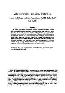
Table 1 shows the descriptive statistics of my main independent and dependent variables. The perceived ﬁne in the baseline and followup surveys (as well as the change in the perceived ﬁne) by poverty level and treatment status are shown in Panel A. In the baseline survey, the average respondent reports that the ﬁne for not voting is S/.121.9, which is close to its old level (S/.144). This conﬁrms that the majority of voters in my sample were not informed about the law that modiﬁed the value of the ﬁne. Importantly, there are no signiﬁcant baseline diﬀerences the perceived ﬁne between the treatment and control group. Fig. 1 shows the distribution of the perceived ﬁne in the baseline and follow-up surveys, for the control and treatment group, by poverty level of the district where each respondent is registered to vote. The distributions in the left column conﬁrm that, not only there were no signiﬁcant baseline diﬀerences in the perceive ﬁne on average, but also the distributions are similar. Exposure to the treatment aﬀected the beliefs about the ﬁne for abstention reported in the follow-up survey. Even though the reduction in the perceived ﬁne is signiﬁcantly larger for voters in the treatment group, there seem to have been within village information spillovers, and thus the distribution of perceived ﬁnes in the control group also shifted to the right, as shown in Panel A of Table 1 and the plots in the right panel of Fig. 1. This was particularly the case for voters in extremely poor municipalities, for whom the average change in the perceived ﬁne is not signiﬁcantly diﬀerent between treatment and control groups.10 Panel B in Table 1 shows that 94.2 percent of the respondents in my sample voted in the October 2010 elections.11 Treatment assignment led to lower turnout. On average, respondents in the treatment group were 3.1 percentage points less likely to vote. This result can be interpreted as a reduced form eﬀect, or the direct (unconditional) eﬀect of the treatment on turnout. The magnitude of this eﬀect is roughly proportional to the reduction of the perceived ﬁne. In non-poor districts, treatment assignment led to a 2.1 percentage points reduction in turnout. Likewise, in poor districts, where the reduction in the ﬁne was larger, treated voters were 5.4 percentage points less likely to vote. Treated voters in extremely poor districts, where the ﬁne was reduced the most, are only 1 percentage point less likely to participate than those in the control group, and the diﬀerence is not statistically signiﬁcant. In these districts, the treatment did not diﬀerentially aﬀect voter's perceptions of the change in the ﬁne, i.e. voters in the control group updated their priors about the ﬁne as much as those in the treatment group, and thus there is no diﬀerence in their voting behavior (on average). The lack of a “ﬁrst stage” for this group does not allow me to do any valid inference from the diﬀerential behavior of the treatment and controls in these municipalities, and therefore in all the subsequent analysis I exclude them and refer to the sample of

According to the information that you just provided me, if you do not vote in the upcoming elections you will be subject to a ﬁne of S/ .[AMOUNT IN THE DISTRICT WHERE SHE'S REGISTERED].To avoid diﬀerential salience of compulsory voting, the control group received a reminder that voting is mandatory and that there is a ﬁne for not voting (without mentioning the amount). The script for the control group was as follows (see Fig. A.1 in the Appendix for Spanish version of both scripts): Dear Sir/Madam, Remember that voting is mandatory in Peru and not voting is subject to a sanction that implies a ﬁne.In practice, the script for the control group did not provide any new information, since in the baseline survey 94.5 percent of respondents reported knowing that voting was compulsory, and that abstention was penalized with a ﬁne.

3.2. The data The baseline interview took place between one and four weeks before the municipal election. We asked for information on household characteristics, household composition and expenditures. Also, we asked about basic demographics, political preferences, policy priorities for the district, knowledge about the current electoral process and past voting. One key variable collected in the baseline survey is the voter's prior about the value of the ﬁne for abstention. To do this, we ﬁrst asked whether the respondent knew if there were any consequences for not voting, and if she responded yes, we followed up asking about the consequences (open question). When the respondent mentioned a ﬁne, we inquired about the amount. I assume that the reported value of the ﬁne is the voter's ex-ante perceived ﬁne.9 At the end of the interview the enumerator provided the treatment. The follow-up survey was collected between one and three weeks after the election. In this survey, we asked again questions on political preferences, political information and interest in politics. The main variables in the survey were whether or not each respondent voted in the municipal election and their perceived ﬁne. The latter was collected using the exact same string of questions as in the baseline, and the perceived ﬁne in the follow up is assumed to correspond to the information each voter had at the moment of the election (when they decided whether to vote or not). I measure voting through both an

10 Overall, it is unclear why information about the new levels of the ﬁne spread more rapidly in these localities. Learning about the new levels of the ﬁne is independent of the size of the village and the number of days between the baseline and follow-up surveys is not statistically diﬀerent between non-poor, poor and extremely poor municipalities (30 days, on average). 11 There are two reasons why turnout in my sample is higher than the oﬃcial statistics: (i) I only sampled voters between 18 and 70 years old, whereas the oﬃcial turnout rate is computed among all registered voters, including voters older than 70 (who are no longer mandated to vote), (ii) conversations with government oﬃcials suggested that the electoral roster is not updated often, thus there are a number of dead people who's names haven't been removed (and of course, they are absent on Election Day).

9 4% of respondents did not know what were the consequences of abstention and 1.3% do not mention a ﬁne as one of the consequences. I assume that they perceive that the ﬁne for abstention is zero. In the few cases in which enumerators were not able to asses an exact value of the perceived ﬁne, respondents were asked to place their beliefs in brackets. For these observations, I use the median value of that range speciﬁed using data from those who did mention an exact value. The main results from the paper do not change if I restrict the sample to only respondents who reported an exact number for the ﬁne, or if I include an interactive term between the variable of interest and a dummy for having provided a range instead of an exact number.

59

Journal of Development Economics 127 (2017) 56–71

G. León

Table 1 Turnout and perceived fine, by treatment and poverty status. Obs.

Total

Treatment

Control

T-C

P-value

PANEL A: Perceived Fines Baseline Non-Poor Poor Extreme Poor

850 882 541

126.85 121.74 115.30

124.57 121.90 111.35

129.30 121.58 119.32

−4.73 0.32 −7.97

(0.18) (0.93) (0.13)

Total

2273

121.93

120.01

123.85

−3.85

(0.12)

Follow-up Non-Poor Poor Extreme Poor

850 882 541

76.84 55.56 27.16

65.88 41.36 19.14

88.43 68.82 35.32

−22.55 −27.47 −16.19

(0.00) (0.00) (0.00)

Total

2273

56.76

45.45

68.05

−22.60

(0.00)

Change Non-Poor Poor Extreme Poor Total

850 882 541 2273

76.84 55.56 27.16 -65.17

65.88 41.36 19.14 -74.55

−22.55 −27.47 −16.19 -18.75

(0.00) (0.00) (0.00) (0.00)

Non-Poor Poor Extreme Poor

850 882 541

0.948 0.941 0.935

0.938 0.913 0.930

0.959 0.967 0.940

−0.021 −0.054 −0.010

(0.175) (0.001) (0.641)

Total

2273

0.942

0.927

0.958

−0.031

(0.002)

88.43 68.82 35.32 -55.80 PANEL B: Turnout

Notes: The changes in the value of the ﬁne established in the 2006 law were: (i) Non-poor districts, S/.72 (from S/.144 to S/.72); (ii) Poor districts, S/.108 (from S/.144 to S/.36); and Extremely Poor districts, S/.126 (from S/.144 to S/.18). The sample comprises all respondents with information on all relevant covariates in the baseline and follow up surveys. For details on the survey questions used to asses the perceived ﬁne, see Subsection 3.2.

voters in poor and non-poor districts as the Analysis Sample.12 The descriptive statistics for the analysis sample by treatment and control status are reported in Table 2. Overall, we observe marginal diﬀerences between the baseline characteristics of these groups, and the test for joint signiﬁcance of the covariates rejects the null at the 95 percent. On average, 40 percent of the sample is male, they are 38.7 years old, with 10 years of education and spend S/.288.1 (∽US$110) per capita per month. Even though the time between the baseline and follow-up surveys was short (30 days, on average), in the analysis sample we were able to track down 1,733 individuals from 1,166 households. Table A.2 shows the balance of observables between attrited individuals and those who we were able to track. Overall, the sample of attriters is not statistically diﬀerent from non-attriters along most of the observable characteristics.13 In the next section, I perform robustness checks showing that attrition is not correlated with treatment status and that any diﬀerential attrition does not signiﬁcantly aﬀected the qualitative or quantitative results in the paper.

about lower levels of the ﬁne on turnout, and identify the main result of the paper, the reduced form eﬀects. Then, after documenting that treatment assignment had an eﬀect on the changes in the perceived ﬁne, I use a 2SLS approach to interpret the magnitude of the reduced for coeﬃcients, and identify the eﬀect of the reduction in the cost of abstention on turnout. 4.1. Reduced form results The reduced form regression identiﬁes the direct eﬀect of informing voters about the new value of the ﬁne on turnout:

Voteikj = α + β1Treat*NonPoorikj + β2Treat*Poorikj + β3Poorij + γXikj + δk + ηikj

(1)

Voteikj is an indicator of whether voter i, living in village/centro poblado k and registered to vote in district j, voted. The treatment status is given by the indicator variables Treat*NonPoorikj and Treat*Poorikj , representing whether voter i was assigned to the treatment group in a Non-Poor or Poor municipality, respectively, and therefore was informed about a reduction in the ﬁne to S/.72 or S/.36. The inclusion of a dummy indicating the level of poverty of the district where the voter is registered to vote allows restricting the comparison to treatment and control units within the same poverty status/level of the ﬁne, NonPoorij is the excluded category. Xikj is a vector of individual level characteristics that are likely to aﬀect voting decisions: gender, age, years of education, and the log per capita expenditures. Finally, δk is a ﬁxed eﬀect at the level of the village where the respondent lives. ηikj is the error term, which I cluster at the level of treatment assignment (the household). It is not straight forward that we should expect changes in the ﬁne to cause lower turnout. Compulsory voting laws have an expressive value beyond any monetary consequences (Funk, 2007). In the

4. Empirical strategy and results The empirical strategy to estimate the eﬀects of being informed about a reduction in the ﬁne on turnout follows directly from the experimental design. First, I exploit the exogenous variation treatment assignment to identify the eﬀects of being exposed to information 12 This sample comprises 1,732 voters instead of the 2,350 shown in Table 1. All the qualitative results from the paper go through if I include this group of the population and a full set of tables is available upon request. 13 One variable that shows systematic imbalances is gender. Men are less likely to be in the follow up survey. Excluding this variable, a joint F-test of the signiﬁcance of the diﬀerence between covariates does not show overall imbalances. In all regressions gender is included among the controls in the regressions to account for this imbalance.

60

Journal of Development Economics 127 (2017) 56–71

G. León

Fig. 1. Perceived ﬁnes, by treatment and poverty status.Notes: Kernel density estimates of the perceived value of the ﬁne for abstention, as reported in the baseline and follow-up surveys. The data in the ﬁgures in the left panels come from the baseline survey and the vertical lines indicate the “old” levels of the ﬁne (S/.144); the information in the right panels comes from the follow-up survey, and the vertical lines denote the value of the “new” ﬁne for each poverty category. For details on the survey questions used to asses the perceived ﬁne, see Subsection 3.2.

tional diﬀerences from Panel B of Table 1. These reduced form eﬀects are consistent with the hypothesis that the cost of abstention is an important determinant of turnout.

Peruvian context, where mandatory voting has been in place for more than 80 years and turnout is consistently high, habit formation (e.g. Gerber et al., 2003, Fujiwara et al. 2014) or social pressure (e.g. Gerber et al., 2008; Funk, 2010) might dominate the eﬀects of the reduction in the ﬁne. Column (1) in Table 3 presents the reduced form estimates of the eﬀects of treatment assignment on turnout (ITT). Being informed about a lower ﬁne reduces the likelihood of voting, and when the information conveys a larger reduction of the ﬁne, the probability of voting is even lower. Treated voters in non-poor municipalities are 2.6 percentage points less likely to vote than the controls in this poverty category. Likewise, voters in poor districts, where the ﬁne was reduced to one fourth of the original amount, showed up at the polls 5.3 percentage points less often than the ones in the control group. Noticeably, these eﬀects are almost exactly the same as the uncondi-

4.1.1. Robustness Attrition rates were not trivial in the experiment, with about 15% of households not present in the follow-up survey. Even though attriters do not look diﬀerent than non-attriters in most observable characteristics (only three out of 21 variables are signiﬁcantly diﬀerent, see Table A.2), if (conditional on observables) attrition is correlated with the treatment, it could partially account for the results observed. Column (1) in Panel A of Table 4 shows that, controlling for individual level observables and village ﬁxed eﬀects, respondents assigned to the treatment are not more likely to be absent at the moment of the follow61

Journal of Development Economics 127 (2017) 56–71

G. León

Table 2 Balance between treatment and control groups. Variable

Perceived Fine (Baseline) Gender (Male=1) Age Yrs. of education PC Expenditures Center Left Right Policy Extreme 1 (Pub. goods) Policy Center Policy Extreme 2 (Club goods) Very Interested in politics Interested in politics Not Interested in politics Very Interested in the results of this election Interested in the results of this election Not Interested in the results of this election Very Interested in the campaign of this election Interested in the campaign of this election Not Interested in the campaign of this election Name recall- Candidates running Name recall- Parties running Name recall- Candidates+Parties running Political information score

Full Analysis Sample

Treatment

Control

Obs.

Mean

Std. Dev.

Obs.

Mean

Std. Dev.

Obs.

Mean

Std. Dev.

1732 1732 1732 1732 1732 1665 1665 1665 1732 1732 1732 1713 1713 1713 1732 1717 1732 1714 1714 1714 1732 1732 1732 1732

124.00 0.40 38.66 10.02 288.08 0.71 0.08 0.22 0.15 0.59 0.26 0.07 0.47 0.46 0.38 0.46 0.16 0.09 0.55 0.35 0.36 0.29 0.33 0.55

54.54 0.49 13.13 3.93 346.28 0.46 0.27 0.41 0.36 0.49 0.44 0.26 0.50 0.50 0.49 0.50 0.37 0.29 0.50 0.48 0.36 0.32 0.32 0.17

863 863 863 863 863 832 832 832 863 863 863 854 854 854 863 858 863 853 853 853 863 863 863 863

122.74 0.41 38.51 10.05 300.99 0.68 0.09 0.22 0.14 0.58 0.28 0.07 0.48 0.45 0.39 0.47 0.14 0.09 0.57 0.33 0.36 0.28 0.32 0.56

53.08 0.49 13.06 3.85 400.01 0.47 0.29 0.42 0.35 0.49 0.45 0.26 0.50 0.50 0.49 0.50 0.34 0.29 0.49 0.47 0.35 0.32 0.32 0.17

869 869 869 869 869 833 833 833 869 869 869 859 859 859 869 859 869 861 861 861 869 869 869 869

125.25 0.40 38.81 10.00 275.27 0.73 0.06 0.21 0.16 0.61 0.23 0.07 0.45 0.48 0.37 0.45 0.18 0.09 0.54 0.37 0.36 0.30 0.33 0.55

55.97 0.49 13.21 4.00 282.66 0.45 0.24 0.41 0.37 0.49 0.42 0.26 0.50 0.50 0.48 0.50 0.38 0.29 0.50 0.48 0.36 0.33 0.33 0.17

T-C

P-value

−2.51 0.01 −0.30 0.05 25.72 −0.04 0.03 0.01 −0.02 −0.03 0.05 0.00 0.02 −0.03 0.02 0.02 −0.04 0.00 0.04 −0.04 −0.00 −0.01 −0.01 0.01

(0.34) (0.64) (0.63) (0.78) (0.12) (0.05) (0.01) (0.54) (0.28) (0.20) (0.02) (0.90) (0.30) (0.27) (0.29) (0.37) (0.02) (0.88) (0.12) (0.08) (0.78) (0.35) (0.54) (0.42)

Notes: The table includes all subjects interviewed in the baseline and follow-up surveys who are considered in the analysis sample, i.e. voters registered in poor or non-poor districts. The test of joint signiﬁcance between treatment and control for voters in rejects the null at the 0.95 (χ2=28.74).

up survey.14 Despite the insigniﬁcant coeﬃcient, its magnitude is not trivial, and thus, to further alleviate concerns about diﬀerential attrition, in Panel A of Table 4 I perform a bounding exercise following Lee (2009). This procedure estimates the upper and lower bounds of the eﬀect of the treatment on the main outcome variable assuming the best and worst case scenario about the voting behavior of the attriters, i.e. that all the diﬀerential attrition is either composed of voters or of abstainers.15 Column (2) shows the unconditional eﬀect of the treatment on voting in the full sample, while columns (3) and (4) show the results of the bounding exercise. The estimate for the lower bound is extremely close to the one for the full sample and still signiﬁcantly diﬀerent from zero, while the upper bound is about 65 percent larger (and statistically signiﬁcant) showing that attrition is not likely to be major concern for my main results. The dependent variable is constructed based on a combination of objective and self-reported measures of voting, which raise concerns about potential biases. First, individuals who show their ID might have diﬀerent observable or unobservable characteristics that could be correlated with voting.16 In Panel B of Table 4 I show the results from the main speciﬁcation using both self-reported and objective measures of voting as a dependent variable. The results are very similar across the diﬀerent samples and voting measures. In the sample for which I

have both self-reported and objective voting measures (comparable sample, in the table), turnout is higher, since people who reported not having voted were less likely to show their ID. The results using the self-reported measure of voting is slightly attenuated, but still large and economically signiﬁcant. Second, if the treatment diﬀerentially aﬀected the probability of showing the ID card, this could introduce bias. Column (1) of Panel C in Table 4, regresses the probability of showing the ID on the treatment variables and the same controls as above, obtaining point estimates very close to zero and statistically insignificant. As with the case of attrition, one might worry that diﬀerential rates of showing the ID card to the enumerator aﬀect my main results, and thus as an additional robustness check, I compute the Lee (2009) bounds for the (unconditional) reduced form eﬀects using only the information of those who showed their ID cards. The lower bound is 40 percent smaller than the eﬀect for the full sample and is statistically insigniﬁcant, however one must take into account that the assumptions used to compute these bounds are quite extreme, especially in a context where turnout is high. One the other hand, the upper bound computed is very close to the eﬀect observed in the full sample. I thus conclude that by using the combination of the objective and self-reported measures of turnout is unlikely to aﬀect my results.

4.2. 2SLS results

14

The unconditional correlation between the treatment and attrition is statistically signiﬁcant, with slightly more attriters among treated respondents. However, this diﬀerence dissapears once I control for observables (and especially the ones that are imbalanced in Table A.2, which are included in the main regressions) showing that attrition should not aﬀect my main estimates. 15 The attrition rate in the treatment group is 21.75 percent, while in the control group, it is 17.77 percent. The estimation of the lower bound is equivalent as saying that any additional treatment non-respondant in the sample would be equivalent to control observations in the lower part of the distribution of the outcome variable (i.e. voters). Similarly, the upper bound is computed assuming that any additional treatment nonrespondants correspond to non-voters in the control group, so I trim them from the control group. The estimation does not allow to include controls in the regressions and the standard errors shown are bootstrapped. 16 Table A.3 in the Appendix shows that the observable characteristics of respondants who showed their ID or not are mostly similar, and a test for the equality of all the variables rejects the null hypothesis of equality at the 95% conﬁdence.

Now that we have established that informing voters about a reduction in the ﬁne aﬀects their voting behavior, and moreover, those voters who received information about a larger reduction in the ﬁne voted less often, it is important to interpret the magnitude of voters' responses, thus in this section, I use a 2SLS model to estimate the cost elasticity of voting. Voters update their beliefs diﬀerentially, even within the same treatment conditions. In order to be able to say something about the magnitude of voter's response to diﬀerent changes in the ﬁne for not voting we need to scale the reduced form eﬀects by the change in the perceived ﬁne caused by the treatment. The ﬁrst stage regression estimates exactly this: 62

Journal of Development Economics 127 (2017) 56–71

G. León

perceived ﬁne (instrumented by the treatment dummies) on turnout:

Table 3 Main regression results. Reduced form

Voteikj = α + β1▵Fineikj + β2Poorij + γXikj + δk + εikj First stage

2SLS

β1 represents the marginal eﬀect of a change of S/.1 in the ﬁne for abstention on the likelihood of voting. The 2SLS results are presented in column (3) of Table 3. An exogenous decrease of S/.1 in the ﬁne for abstention reduces the likelihood of voting by 0.17 percentage points. Using these estimates, I can back out the cost-elasticity of voting. The average voter in the analysis sample reports that the ﬁne was reduced by S/.58 (46.8 percent from the baseline perception of S/.124), hence the eﬀect of the drop in the perceived ﬁne on turnout for the average voter is −9.86 percentage points (10.43 percent). These results imply that the observed reduction in the perceived ﬁne lead to a drop in turnout from 94.5 to 84.6 percent and a cost-elasticity of −0.22. Column (4) of Table 3 presents a validity test for the eﬀect of the treatment on turnout. If the treatment did aﬀect the perceptions about the magnitude of the ﬁnes, it should have aﬀected turnout in 2010, but it had no way of aﬀecting past behavior. The change in the perceived ﬁne do not have a statistically signiﬁcant eﬀect on the self-reported measure of voting in 2006 and the coeﬃcients are very close to zero, providing support to the assumption that voters in the treatment groups were not already less likely to vote than those in the control group in previous elections. Extrapolating these results to the whole population (with the obvious caveats), a reduction in the ﬁne of 50 percent would reduce turnout in about 11 percentage points, while driving the ﬁnes to zero could lead turnout to 72.5 percent, a level comparable to the one observed in some countries where voting is voluntary. To put these results in context with the previous evidence, Gerber et al. (2008) ﬁnd that reminders to vote emphasizing social pressure messages cause an increase in turnout between 4.8 and 8.1 percentage points.18

Dependent Variable: Voted in the 2010 Election

Perceived fine (follow-up)

▵ Perceived Fine

Treatment: Fine S/.72

Treatment: Fine S/.36

Controls Village FE Mean Dep. Var. First Stage Fstat Obs.

−.026

−17.420

(0.015)

(4.851)***

−.053

−28.848

(0.016)***

(4.644)***

Y Y 0.944

Y Y −58.00

1732

1732

Voted in the 2010 Election

Voted in the 2006 Election

0.0017

0.00008

(0.0005)***

(0.0005)

Y Y 0.944

Y Y 0.945

25.63

20.84

1732

1548

Robust standard errors clustered at the household level in parentheses. Column (1) presents a linear probability model, while in Column (2) I use OLS, and in Column (3) and (4), I present 2SLS regressions where Δ Perceived Fine is instrumented by the two treatment dummies (Treat*NonPoor and Treat*Poor). Regression equations are speciﬁed in Eqs. (1), (2) and (3). The sample size in Column (4) is smaller than the analysis sample because there are a number of voters in the sample who voted for the ﬁrst time in 2010. All regressions include controls for gender, age, years of education, log(PC Expenditures), and a dummy for being registered to vote in a poor district. The overidentiﬁcation test is unable to reject the joint null hypothesis is that the instruments are valid instruments (Sargan test with a p-value=0.7649; Basmann test p-value=0.7673). * Signiﬁcant at 10%; ** Signiﬁcant at 5%; *** Signiﬁcant at 1%.

4.2.1. Interpretation of the 2SLS results and the exclusion restriction The interpretation of my 2SLS estimate as the cost elasticity of the ﬁne relies on the assumption that the information treatment only aﬀected turnout through the change in the perceived ﬁne. One concern is that the information also aﬀected the perceived enforcement probability. If voters in the treatment group perceived that, by reducing the ﬁne for abstention, the government is signaling that voting is less important and thus reducing enforcement, voters in the treatment group would have a lower expected value of the ﬁne driven by the both, the lower perceived ﬁne and enforcement. In the follow-up survey I asked voters to name all the possible consequences of abstention, this is, which services they believed they would be denied access to in case of abstention. In the ﬁrst six regressions of Table 5, I regress the perceived consequences of not voting on the treatment variables and the controls used in the previous analysis. All coeﬃcients are very close to zero and are statistically insigniﬁcant, showing that voters in the treatment group are not less likely to think that the chances that they are denied a particular service are higher than those in the control group. A potential violation of the exclusion restriction would happen if the treatment diﬀerentially aﬀects the salience of the importance of voting. To test whether this is the case, I follow a similar strategy as before, and run my main speciﬁcations, but using as the dependent variable proxies for the perceived value of voting, measured in the follow-up survey, eg. the importance of the elections and the electoral campaigns. The results in the last two columns of Table 5 show that the treatment did not diﬀerentially aﬀect the voters' value of elections.19

▵Fineikj = α + β1Treat*NonPoorikj + β2Treat*Poorikj + β3Poorij + γXikj + δk + νikj

(3)

(2)

▵Fineikj = (Fine2 − Fine1)ikj is the change in the perceived ﬁne between the follow-up and baseline surveys.17 β1 and β2 represent the diﬀerence in the average change in the perceived ﬁne between the treatment and control groups, among voters from non-poor and poor municipalities, respectively. The results from the ﬁrst stage regression are displayed in Column (2) in Table 3. The diﬀerence in the change in perceived ﬁne for the treatment and control groups is S/.17.4 in non-poor municipalities, while the treatment eﬀect for voters in poor districts is a reduction in the perceived ﬁne of S/.28.8. Treatment assignment aﬀected the beliefs about the ﬁnes in the way we expect them, but the magnitude of the changes between the treatment and control groups is lower than the actual changes in the ﬁnes, which is potentially a result of the information spillovers described in Section 3.3. These results provide a strong ﬁrst stage for 2SLS strategy, with an F-statistic for the excluded instruments of 25.6. In the second stage, I analyze the eﬀect of the changes in the

17 The main regressions in the paper use a speciﬁcation in which I focus on the eﬀects of ΔFine on voting, rather than the eﬀect of Fine2. The reason behind this choice is because there seems to be anchoring in the way individuals update their beliefs about the ﬁne, and this is particularly the case among those in the control group, for whom the correlation between Fine1and Fine2 is 0.14 (statistically signiﬁcant). This leads us to believe that accounting for the diﬀerential updating in the ﬁrst stage is important. However, all the results in the paper remain quantitatively and qualitatively unchanged if I did not include Fine1 in the regression equation. A full set of results is available upon request.

18 The reduced form, ﬁrst stage and 2SLS results remain unchanged if we include in the estimation voters from Extremely Poor municipalities, as shown in Panel A of Table A.4. Likewise, most of the qualitative results of the paper go though if I include these observations. These results are available upon request. 19 Another threat along the same lines is that the treatment induced lower information acquisition and thus aﬀected turnout. In Table 9, Section 6, I show evidence that voters in the treatment group did not acquire less political information than those in the control group.

63

Journal of Development Economics 127 (2017) 56–71

G. León

Table 4 Robustness checks: attrition and measurement of voting. Panel A: Attrition Lee (2009) Bounds Dep. Var: Voted in the 2010 Election

Dep. Var: Attrited

Full Sample

Lower Bound

Upper Bound

Treatment

0.043 (0.0282)

−0.037 (0.0113)***

−0.035 (0.0126)***

−0.062 (0.0204)***

Controls Village FE Mean dep. var. Obs.

Y Y 0.218 2214

N N 0.944 1732

Benckmark

N N 0.944 2214 Panel B: Diﬀerent Measures of Turnout Dep. Var: Voted in the 2010 Election Available Sample Self Reported Sticker

Comparable Sample Self Reported

Sticker

▵ Perceived Fine

0.0017 (0.0005)***

0.0014 (0.0005)***

0.0011 (0.0005)**

0.0016 (0.0005)***

Controls Village FE Mean dep. var. F-statistic Obs.

Y Y 0.944 25.627 1732

Y Y 0.944 25.248 1729

Dep. Var: Not Showed ID

Full Sample

Treatment

−0.0183 (0.0243)

−0.0352 (0.0101)***

−0.0192 (0.0179)

−0.0365 (0.0119)***

Controls Village FE Mean dep. var. Obs.

Y Y 0.347 1732

N N 0.971 1130

N N 0.971 1732

N N 0.971 1732

0.0015 (0.0005)***

N N 0.944 2214

Y Y Y Y 0.971 0.971 15.573 15.148 1130 1127 Panel C: Measurement of Voting Lee (2009) Bounds Dep. Var: Voted in the 2010 Election (Sticker) Lower Bound

Y Y 0.971 15.148 1127

Upper Bound

Robust standard errors clustered at the household level in parentheses. In Column (1) of Panel A, I use and OLS regression. Columns (2)–(4) I run the reduced for regression without controls or fixed effects, dropping some observations from the control group under different assumptions, following Lee (2009). In Panel B, all linear probability models follow the same structure as in Eq. (3), including controls and village ﬁxed eﬀects. The dependent variables are self reported or objective measures of turnout. Columns (1)–(3) use all the analysis sample for which the dependent variable is available. Column (1) presents the benchmark speciﬁcation from Table 3, Columns (2) and (3) use as dependent variables a self reported and objective (i.e. Sticker) measure of turnout, respectively. Columns (4) and (5) repeat the exercise from Columns (2)–(3), but restricting the sample to voters for whom both outcomes are observed (i.e. Comparable sample). In Panel C, Column (1) uses an OLS model with controls and ﬁxed eﬀects. Columns (2)–(4) are analogous to those in Panel A. * Signiﬁcant at 10%; ** Signiﬁcant at 5%; *** Signiﬁcant at 1%.

The spread of information about the new level of the ﬁne between the treatment and the control group represent a threat to the interpretation of my estimates as long as this information was acquired before the election (otherwise, this information wouldn't have aﬀected voting decisions). Table 6 explores the correlation between the number of days between the baseline and follow-up survey and Election Day, and the changes in the perceived ﬁne. As expected, the time between surveys is only signiﬁcantly related to changes in the perceived ﬁne among control households (the treatment group received the information just after the baseline survey). Interestingly, learning in the control group seems to have happened after the election and not between the baseline and the election. This means that most voters in the control group had not updated their information about the changes in the ﬁne by the time they made the decision of whether to vote or not. The evidence from Table 6 suggests that the perceived ﬁne reported by controls in the follow-up should be taken as an upper bound of their beliefs about the ﬁne and the estimates in the regressions, as lower bounds. The results in Column (3) of Table 3 can be interpreted as the local average treatment eﬀects (LATE) of a marginal reduction in the cost of abstention on voters whose priors about the ﬁne were updated by the treatment. This interpretation relies on assumptions on how people update their information sets under diﬀerent treatment conditions, i.e.

I assume that the treatment leads everyone to update their beliefs about the ﬁne in the same direction. If the monotonicity assumption does not hold, the interpretation of the 2SLS results as LATE would be threatened, in which case, the IV estimator is not guaranteed to estimate a weighted average of the underlying individual causal eﬀects and the LATE would not converge to the IV estimator (Angrist and Pischke, 2009, pp. 154–158). More precisely, in our case, the monotonicity assumption implies that, compared to the counterfactual, all voters in the treatment group should update their beliefs downwards (ΔFi ≤ 0 ), i.e. otherwise, this might imply the presence of deﬁers in the sample. Even though the presence of deﬁers is an untestable assumption, I can provide evidence that, if they were present, this would not generate a signiﬁcant biases to my main estimates. One group in the analysis sample where we might ﬁnd deﬁers is among voters whose initial beliefs about the ﬁne were below the new level. 11 percent of voters in the analysis sample fall in that category. In terms of the potential outcomes framework, this 11 percent (besides deﬁers) can also include never takers. Panel B in Table A.4 in the Appendix presents the main regressions of the paper excluding this group of voters. The point estimates in the reduced form, ﬁrst stage, and 2SLS regressions are remarkably similar to those in Tables 3, providing evidence that either there are few deﬁers in the sample or that their presence would not bias my estimates.

64

Journal of Development Economics 127 (2017) 56–71

G. León

Table 5 Effect of the treatment on perceived consequences of abstention.

Treatment: Fine S/.72 Treatment: Fine S/.36

Controls Village FE Mean dep. var. Obs.

Treatment: Fine S/.72 Treatment: Fine S/.36

Controls Village FE Mean dep. var. Obs.

Fine

Dep. Var: Consequence of Abstaining: Can't use Can't use pubic inst banks (municipality, police, etc.)

Can't use notariat

-.0056 (0.0051) -.0076 (0.0051)

0.0188 (0.0271) -.0023 (0.0218)

0.0108 (0.0209) -.0013 (0.0179)

0.0005 (0.0168) -.0107 (0.0154)

Y Y 0.994 1712

Y Y 0.155 1712

Y Y 0.096 1712

Y Y 0.062 1712

Dep. Var: Consequence of Abstaining: Can't use Other: registry (contracts) (travel, jail, jobs, etc.)

V. Interested in Campaign (Follow-up)

V. Interested in Results (Follow-up)

0.0178 (0.0152) -.0013 (0.0131)

0.0252 (0.0329) 0.0306 (0.0259)

-.0054 (0.0242) -.0109 (0.0271)

0.0399 (0.0344) -.0133 (0.0324)

Y Y 0.047 1712

Y Y 0.287 1712

Y Y 0 .153 1725

Y Y 0.357 1729

* signiﬁcant at 10%; ** signiﬁcant at 5%; *** signiﬁcant at 1%. Robust standard errors clustered at the household level in parentheses. All 2SLS models include village ﬁxed eﬀects and controls, and the endogenous regressor is instrumented by the two treatment dummies. The regression equation for the second stage is given by: Consequence ikj = α + β1Treat *NonPoorikj + β2Treat *Poorikj + β3Poorij + γXij + δk + ηikj .

Finally, one might be worried that the choice of the main independent variable could aﬀect the results. Table A.7 in the Appendix shows the results of the main IV regression using as the endogenous regressor, instead of ΔFij , the level of the perceived ﬁne in the follow-up (in levels or logs, while controlling for the baseline perceived ﬁne), or the ﬁne as a percentage of per capita expenditures. The quantitative and qualitative results are robust to the choice of the independent variable.

Table 6 Spread of information and days between surveys. Dep. Var.: ▵ perceived ﬁne Treatment

Control

Num. days: Baseline-Election

−.0841 (0.2243)

−.0916*** (0.2728)

Num. days: Election-Followup

−.0336

−2.6682

(0.4156)

(0.4573)***

862

868

Num. days: Baseline-Followup

5. Political preferences, value of voting, and information The reduced form and 2SLS results show that exposure to the treatment had impacts on turnout, and that the magnitude of the change in the ﬁne signiﬁcantly aﬀected participation. However, to understand the eﬀects of the cost of abstention on preference aggregation and its potential impacts on public policies, we need to look beyond the eﬀects on the level of turnout and dig further into what happens with the composition of the electorate. The identity of the marginal voter and her preferences determine whether changes in turnout will translate into substantial eﬀects on who gets elected and what policies get implemented. Theoretical models in the literature (see e.g., Martinelli, 2005; Merlo, 2006 for critical reviews) use a few common dimensions of heterogeneity among voters: (i) ideological positions, (ii) subjective value of voting and (iii) political information. In this section, I analyze the heterogeneous eﬀects of the changes in the cost of abstention to qualify the identity of marginal voters who responded to the policy. Using the 2SLS framework from the previous section, I introduce in my main regression interactive terms between the (instrumented) change in the perceived ﬁnes and variables that proxy for the relevant characteristics being evaluated (while controlling for the others).

Obs.

Treatment

Control

−.0719

−.7557

(0.2003)

(0.242)***

862

868

Robust standard errors clustered at the household level in parentheses. OLS regressions include dummies for poverty category. * Signiﬁcant at 10%; ** Signiﬁcant at 5%; *** signiﬁcant at 1%.

ferences usually assume that those with more intense preferences (i.e. extremists) will be more likely to vote than centrists. However, if voters have uncertainty about the candidate's position and can make voting mistakes (see eg. Degan, 2006; Degan and Merlo, 2011), or in models based on strategic extremism (Glaeser et al., 2005), centrists are more likely to participate. In the presence of costly voting, these two broad families of models provide diﬀerent predictions on the identity of the marginal voter who will be aﬀected by changes in the cost of abstention. In local elections it is not straightforward to understand the role played by ideological preferences. While in the Peruvian case, national parties with well deﬁne ideologies compete in these elections, a good part of the candidates are independent, and base their campaigns on speciﬁc proposals rather than in the standard ideological scale, but in

5.1. Ideological positions Models in which voters derive utility from expressing their pre65

Journal of Development Economics 127 (2017) 56–71

G. León

to the polls regardless of the change in the perceived ﬁne, and the magnitude and signiﬁcance of the eﬀect decreases with the interest in politics. A similar pattern is observed when using the alternative proxies for the subjective value of voting. Using the results from Panel B in Table 7 I am able to provide revealed preference estimates of the subjective value of voting. Voters who are less interested in politics are much more sensitive to a change in the ﬁne for abstention, with an elasticity of −0.247. This result implies that in order to increase their probability of voting for this group from the observed 93.5 percent to 100 percent, we would need to increase in the ﬁne for abstention in S/.92.4 (∼US$33). Likewise, voters who are interested in politics have an elasticity of −0.159, hence to achieve full participation among these voters, the ﬁne would have raise by S/.77.4 (∼US$27). Finally, voters who are very interested in politics are hardly sensitive to changes in the ﬁne, with an implied elasticity of −0.13, and they would vote even if the ﬁne was set at zero.

general we see some regularities with, e.g. left leaning candidates proposing public works while right leaning candidates propose to help promote small entrepreneurs. To empirically approximate ideological preferences, I use two distinct measures that are intended to capture these dimensions. First, I use standard self-reports in the ideological scale, ranging from left (1) to right (5) and take the categories in the middle (2, 3 and 4) to represent the political center. As can be seen in Table 2, there is a concentration of voters in the center. Alternatively, I create a second measure that uses policy preferences to capture a broader range of ideological distributions. In the baseline survey, I asked voters to name (in order) the ﬁrst ﬁve policies that they would implement if they were elected mayor of the district. This was an open question and enumerators had to place the answers in one of twenty eight policy categories. For each of these categories, the policy preferences are ordered from not mentioned (zero) to most preferred (ﬁve). I aggregate these questions by taking the ﬁrst principal component and dividing the sample into quintiles of the ﬁrst PC. The center is deﬁned by those in quintiles 2, 3 and 4, while the ﬁrst and ﬁfth quintiles deﬁne the ideological extremes (the coeﬃcients for each policy item loading into the principal component analysis are listed in Table A.5.) The Policy Extreme 1 is related to preferences for public goods, such as health and education infrastructure, roads, etc. On the other hand, Policy Extreme 2 is associated with club or targeted goods, such as youth labor training, security, promotion of private investment, etc. These two variables are meant to represent diﬀerent dimensions in which voters preferences can be represented. Panel A in Table 7 shows the results from estimating Eq. (3), including interactions between the variables representing voter's ideological position and the perceived change in the ﬁne, instrumented by the treatment status and the relevant interactions (I don't include ΔFine in the regression). In Column (1) I use the self-reported measure of political ideology and ﬁnd that the bulk of the eﬀect of the change in the ﬁne on turnout is driven by voters who place themselves in the political center. Voters on both political extremes seem to be unresponsive to changes in the ﬁne for abstention. The results in Column (2) use the second measure of ideological position (based on policy preferences) are even more stark. Voters in the second through fourth quintiles of the policy preference scale account for the whole eﬀect of changes in the ﬁne for not voting, while voters in the political extremes show eﬀects close to zero and statistically insigniﬁcant. Overall, the results from Panel A in Table 7 show that people in the political extremes are less likely to respond to a change in monetary incentives to vote. This result has important implications for thinking about incentives to vote and its potential eﬀects on political competition and social conﬂict. In the medium run, the political supply should respond to changes in the electorate. If this is the case, a reduction in turnout among centrists might lead parties to bunch in the extremes of the political spectrum, which can cause coordination problems, polarization and social conﬂict.

5.3. Political information Are informed voters more or less likely to respond to changes in the cost of abstention? Both common and private values models predict that informed voters are more likely to participate in elections (see, eg. Feddersen, 2004; Degan and Merlo, 2011, among others), hence we should expect uninformed voters to be more likely to abstain upon a reduction in the ﬁne. In this subsection, I test this empirically by interacting diﬀerent measures of political information collected at baseline with the change in the perceived ﬁne. Political knowledge and information about politics are measured in several ways. In the baseline survey, I included open ended questions asking respondents to name all candidates running for the mayor's seat in the municipality where they are registered to vote (and their parties). All measures of political information are expressed as ratios of the number of candidates (and/or parties) that the respondent is able to name as a proportion of the total number of candidates (and/or parties) running for oﬃce. The average respondent in the analysis sample is able to name 36 percent of the candidates and 29 percent of the parties they are running for. As an alternative measure of political information, I asked 17 questions about knowledge of the political structure of the country, electoral institutions and rules.20 The average respondent got 9.3 questions right (55 percent). Importantly, these political information measures are uncorrelated with the baseline knowledge about the ﬁne. For instance, the correlation between the absolute value of the error in the perceived ﬁne at baseline (—perceived - actual ﬁne—) and the index of knowledge of candidates is 0.0005. Panel C in Table 7 shows the results of running Eq. (3) including the interactions between the perceived change in the ﬁne and our measures of political information. In all four columns, the interactive terms are negative and signiﬁcant, meaning that people who have higher levels of information are less likely to change their turnout decision when they learn that the ﬁne has been reduced. Moreover, fully informed voters are unaﬀected by the changes in the ﬁne. Previous evidence shows that more informed voters are more likely to hold the elected oﬃcials accountable and less likely to elect corrupt politicians (e.g. Ferraz and Finan, 2008; Banerjee et al., 2011; Pande, 2011.) It is possible that by reducing the cost of not voting and allowing less informed voters to select out of the voters' pool, we could increase the quality of elected oﬃcials. Despite the fact that the independent results of the heterogeneity analysis are consistent with several theoretical models in the literature, few predict at the same time that voters who are more likely to respond

5.2. Interest in politics/subjective value of voting Models of expressive voting suggest that voters with a higher subjective value of voting need lower incentives to attend to the polls. The subjective value of voting is an unobserved individual characteristic and I use a battery of questions on interest in politics, in the results of the current election, and in the campaign from the baseline survey to proxy for it. Few people (7 percent) declare themselves to be very interested in politics, while 47 percent are somewhat interested, and 46 percent are not interested at all (see Table 2). The relatively little interest in politics is also apparent from the small proportion of voters who are very interested in the results of the election or in the campaign (38 percent and 9 percent, respectively). In Panel B of Table 7 I run a similar regression as in Subsection 5.1. The results show that voters who are more interested in politics attend

20 The questions include information about the length of the term, reelection possibilities for two consecutive periods, length of the term, and existence of run-oﬀ elections for president, congressmen and mayor, the oﬃcial minimum and maximum age for which voting is mandatory, and which are the government institutions in charge of the elections, ID cards and political claims.

66

Journal of Development Economics 127 (2017) 56–71

G. León

Table 7 (continued)

Table 7 Effect of changes in perceived fine on turnout, by political preferences, interest in politics and information.

Dep. Var: Voted in the 2010 Election −.0081 (0.0045)*

▵ Fine*Pol. Info. Score

Dep. Var: Voted in the 2010 Election PANEL A: Political Preferences

Obs.

▵ Fine*Left

−.0006 (0.0024)

▵ Fine*Center

0.0015 (0.0006)**

▵ Fine*Right

0.001 (0.0008)

▵ Fine*Policy Extreme 1

0.0003 (0.0013)

▵ Fine*Policy Center

0.002 (0.0007)***

▵ Fine*Policy Extreme 2

0.0008 (0.001)

Obs.

1650

▵ Fine*Very interested in politics

0.0003

▵ Fine*Not interested in politics

0.0019

1650

6. Preference aggregation, information acquisition and vote buying

(0.0007)***

▵ Fine*Very interested in results

1650

to changes in the cost of voting are those that (i) are in the political center, (ii) have low subjective value of voting, and (iii) are uninformed. One such model is an extension of the one in Merlo (2006) and Degan and Merlo (2011), which I present in Appendix B. In this model, voters know their political preferences, but are imperfectly informed about the candidate's position. They derive utility from fulﬁlling their civic duty, from voting for the candidate that is closest to their political preferences and from money. Information is exogenous in the model and the fact that voters are imperfectly informed about the candidates makes them prone to make a voting mistake. In this set up, marginal voters, i.e. those who are more likely to respond to a decrease in the cost of abstention will be the centrists, the ones with a lower subjective value of voting and the uninformed.

(0.0017) 0.0012 (0.0007)*

1650

Robust standard errors clustered at the household level in parentheses. Information on political preferences, interest in politics, and political information was collected in the baseline survey. All 2SLS models include village fixed effects, demographic controls, controls for political preferences (right, left), interest in politics (Very interested in politics, interested in politics) and information (Candidate recall), and the endogenous regressor and its interactions are instrumented by the two treatment dummies and the relevant interactions. * Signiﬁcant at 10%. ** Signiﬁcant at 5%. *** Signiﬁcant at 1%.

1650 PANEL B: Interest in Politics

▵ Fine*Interested in politics

1650

0.0007

While the conceptual framework in Appendix B helps us think through the heterogeneity results, the model is silent about the eﬀect of changes in the composition of the electorate on the aggregation of preferences and electoral outcomes. Further, an extension of the model in the appendix can include endogenous information acquisition, as in Degan (2013), and this test is also presented below.

(0.0006)

▵ Fine*Interested in results

0.002 (0.0008)**

▵ Fine*Not interested in results

0.0038 (0.0019)**

6.1. Policy preferences ▵ Fine*Very interested in pol. campaign

0.0023

Electoral institutions in democratic societies are designed to maximize voter representation and to ensure that policies are catered towards the interests of the majority. Mandating citizens to participate in elections imposes a cost on society and it could be justiﬁed if this led to improved representation. Theoretical arguments are mixed. Depending on the assumptions on the type of information available to voters, diﬀerent authors have argued that compulsory voting can be welfare increasing or decreasing. Krishna and Morgan (2014) present a model showing that under voluntary voting, information aggregation holds and mandating people to vote imposes a net cost to society. Along the same lines, Borgers (2004) reaches a similar conclusion based on a model with simple private value majoritarian elections. On the other hand, Ghosal and Lockwood (2009) use a model with common values to show that compulsory voting pareto-dominates voluntary participation. Even though I am not able to directly test the speciﬁc predictions of these models, I can provide evidence to help us think about how diﬀerent incentive schemes to participate in elections aﬀect policy outcomes. One way to address this issue is to analyze if people who prefer certain type of policies are more likely to respond to monetary incentives to vote. If that is the case, a reduction of the ﬁne for abstention will lead to under-representation and thus the policies preferred by this group will not be enacted (assuming perfect commit-

(0.0021)

▵ Fine*Interested in pol. campaign

0.0008 (0.0005)

▵ Fine*Not interested in pol. campaign

0.0029 (0.0011)**

Obs.

1650

▵ Perceived Fine

0.0024 (0.0008)***

▵ Fine*Candidate recall

−.0029 (0.0012)**

▵ Fine*Party recall

▵ Fine*Candidate and Party recall

1654 1651 PANEL C: Political Information 0.0021 (0.0007)***

0.0024 (0.0007)***

0.006 (0.0027)**

−.0026 (0.0011)** −.0032 (0.0012)**

67

Journal of Development Economics 127 (2017) 56–71

G. León

over-represented among those who stop voting due to the treatment. The only interaction coeﬃcient that comes through statistically and economically signiﬁcant is the one for voters who have preferences for policies that promote agricultural activities (i.e. water projects, investment in improved seeds, etc.) This result is related to the literature showing empirically how the enfranchisement of diﬀerent groups of the population leads to changes in policies (Husted and Kenny, 1997; Fujiwara, 2015; Miller, 2008; Naidu, 2012.) However, when the cost of voting is reduced, there is no a priori reason to expect that voters who select out of the pool of voters have diﬀerent policy preferences and thus allowing them to abstain should not lead to signiﬁcant changes in policies. This is consistent with Hoﬀman et al. (2017), who show that the elimination of compulsory voting in Austrian states does not lead to a signiﬁcant change in the composition or levels of expenditures. Overall, these results suggest that the average voter who abstains when facing a lower ﬁne for not voting does not have signiﬁcantly diﬀerent policy preferences than the average voter who still votes despite the reduction in the ﬁne. Assuming perfect commitment by politicians, this implies that the change in the electorate due to lower incentives to vote will not cause a change in the policies implemented by elected oﬃcials.

Table 8 Effects by policy preferences. Dep. Var.: Voted in the 2010 Election Coeff. on ▵ Perceived Fine

Coeff. on ▵ Perceived Fine*Policy

0.002 (0.0008)**

−0.0005 (0.001)

(2) Education

0.001 (0.0006)*

0.0012 (0.0011)

(3) Infrastructure

0.0011 (0.0012)

0.0007 (0.0014)

(4) Order and Security

0.0023 (0.0008)***

−0.0013 (0.0011)

(5) Promote micro-enterprises/ training

0.0017

0.0002

Policy (1) Health

(0.0006)

***

(0.0012)

(6) Agriculture

0.0024 (0.0007)***

−0.0022 (0.0009)**

(7) Youth/Women

0.0014 (0.0006)**

0.0013 (0.0012)

(8) Cleaning/Environment

0.0014 (0.0006)**

0.0009 (0.0011)

(9) Institutions

0.0019 (0.0006)***

−0.001 (0.0011)

(10) Social/work programs

0.0018 (0.0006)***

−0.0004 (0.0011)

6.2. Information acquisition Proponents of mandatory voting argue that mandating people to vote not only increases participation, but also incentivizes people to be more involved in the political process, for example by acquiring information. The underlying model for these claims is one similar to the one Appendix B, but it endogenizes information acquisition (Martinelli, 2005; Degan, 2006, 2013; Oliveros, 2013). The intuition behind these models is that for suﬃciently high penalties for not voting, abstention will drop and people might demand more political information to avoid making a “voting mistake.” In the follow-up questionnaire, I included questions assessing the level of political information held by each respondent, which allow me to test if voters who stop voting due to a lower perceive penalty are less likely to acquire political information. In Panel A of Table 9 I regress the change in the diﬀerent measures of political information on the change in the perceived ﬁne, instrumented by the treatment status. The eﬀect is very close to zero and not statistically signiﬁcant. Voters who stop voting due to a lower costs for abstention do not acquire information diﬀerentially than their peers who face a higher ﬁne. This result is consistent the predictions of the models in Degan (2006, 2013), as well as with the empirical ﬁndings in Loewen et al. (2008) and Leite Lopez de Leon and Rizzi (2014), but contradict those in Shineman (2014), who shows that an increase in political participation leads to more information acquisition. These results must be taken with a grain of salt, since even though around the elections voters are more likely to get informed about the candidates and the political process overall, the average time between surveys was short (30 days). Further, in the medium or long-run people who stop voting might also change their behavior in terms of information acquisition.

Robust standard errors clustered at the household level in parentheses. The coefficients shown in each row come from separate 2SLS regressions models, include village fixed effects and controls, and the endogenous regressor and its interactions are instrumented by the two treatment dummies and the relevant interactions. The table reports the coefficients for the instrumented endogenous regressor and the relevant interaction. Policy preferences include: (1) Health: Infrastructure, health professionals, and training for health workers; (2) Education: Infrastructure, teachers, and training for teachers; (3) Infrastructure: Roads and access to them, sewage, water, electricity and telecommunications infrastructure, build markets, churches, community building, main square; (4) Order and Security: Traffic, more policemen in the streets, fight drugs and gangs; (5) Promote micro-enterprises/training: promote micro/small firms, train local entrepreneurs, promote private investment, promote tourism; (6) Agriculture: Build dams and irrigation infrastructure, technical assistance to agriculture, seed banks, support livestock farmers; (7) Youth/Women: Women empowerment and equality, youth policies, sporting events; (8) Cleaning/Environment: street cleaning, increase green areas, promote recycling; (9) Institutions: Transparency in managing the municipality, fight corruption, modernize the bureaucracy, participatory decision-making, land titling; (10) Social/work programs: Job training programs, help those in poverty, food aid, child care, generate jobs. For each of these categories, the dependent variable is a dummy indicating whether the respondent named at least one of the policies in this category as one of her five priorities for the district. * Signiﬁcant at 10%. ** Signiﬁcant at 5%. *** Signiﬁcant at 1%.

6.3. Vote buying

ment by politicians). To implement this test, I use the policy preference questions, aggregating them into 10 categories that represent particular policy issues and analyze whether voters with speciﬁc policy preferences are more or less likely to respond to changes in the ﬁne. I do this by running my baseline regression in Eq. (3), and interact the (instrumented) change in the perceived ﬁne with a dummy for whether each respondent has a preference of each groups of policies. The results from this analysis are presented in Table 8. The interaction terms between policy preferences and changes in the ﬁne for not voting are not statistically signiﬁcant and very close to zero, suggesting that voters with particular policy preferences are not

Electoral processes in developing countries are often prone to vote buying or turnout buying (Vicente, 2014; Vicente and Wantchekon, 2009; Finan and Schechter, 2012; Stokes, 2009; Stokes et al., 2013; among others.) This speciﬁc type of clientelism generates distortions in the aggregations of preferences, inducing voters to participate or to vote for someone they wouldn't have otherwise by transferring resources from candidates to voters. In my sample, 31 percent of respondents reported having been oﬀered and accepted cash or a gift from a political operator. In electoral systems with compulsory voting, voters who go to the polls because of the mandate are more likely to 68

Journal of Development Economics 127 (2017) 56–71

G. León

the ﬁne for abstention of S/.1 leads to an increase in the price of the vote of S/.0.08. The average voter, who perceived that the ﬁnes were reduced by S/.58, would have to be paid 75 percent more than before to buy her vote. As a robustness check for this result, in Column (3) I use as a dependent variable the amount of money indirectly received by the voter, e.g. in a massive rally. If there is a negotiation between the voter and the political operator about the price of the vote, I do not expect this negotiation to aﬀect the amount received indirectly. Indeed, I ﬁnd a statistically and economically insigniﬁcant eﬀect. Overall, the a reduction in the ﬁne for abstention does not aﬀect the incidence of vote buying, however each vote becomes more expensive, making it more costly to politicians to have inﬂuence on the outcome of the election through vote buying, a result that is consistent with the theoretical framework in Gans-Morse et al. (2013).

Table 9 Effects of fines on information acquisition and vote buying. Panel A: Eﬀect of Fines on Information Acquisition Dep. Var.:

▵ Perceived Fine

Controls Village FE Obs. F-Stat

▵ Perceived Fine

Controls Village FE Mean dep. var. Obs. F-statistic

▵ Candidate

▵ Party

▵ Pol. Info

Recall

▵ Cand. +Party Recall

Recall −.0003

−.0006

−.0004

−.00002

(0.0005)

(0.0006)

(0.0005)

(0.0004)

Score

Y Y 1732 68.57

Y Y Y Y Y Y 1732 1732 1732 68.57 68.57 68.57 Panel B: Eﬀects of Fines on Vote buying Dep. Var: Amount Amount Amount 1=Accepted Money Accepted Accepted Accepted or a Gift Directly Indirectly Total

−.0002

−.0780

0.0105

−.0692

(0.0009)

(0.0388)

(0.0176)

(0.0394)

Y Y 0.310

Y Y 6.48

Y Y 3.22

Y Y 10.08

1732 25.62

537 11.40

537 11.40

537 11.40

7. Summary and discussion Electoral institutions that encourage or mandate citizens to vote are widespread around the world. Such institutions are often introduced in the spirit of democratization, hoping to achieve better representation and to involve citizens in the political process. However, since both voting and enforcing institutions are costly, there could be signiﬁcant welfare losses if the objectives of higher participation and more involvement are not achieved. In this paper I combine a natural experiment provided by a change in Peruvian voting laws with a ﬁeld experiment to identify the eﬀect of ﬁnes for abstention on voting. I ﬁnd that a reduction in the cost of abstention decreases turnout, and that this reduction is more than proportional among (i) centrist voters, (ii) those who have a lower subjective value of voting, and (iii) voters who hold less political information. These results are consistent with the predictions of the rational choice model of voter behavior with imperfect information. The reduced form results show that being informed about a larger reduction in the ﬁne for abstention leads to lower turnout. This results contribute to the literature on the eﬀects of monetary incentives to vote. I interpret the magnitude of these results using a 2SLS model, and show that reducing the ﬁnes for not voting by half leads to a 10 percentage point reduction in turnout. Further, the experimental design allows me to compute the elasticity of voting with respect to the cost, which I ﬁnd to be −0.22. To my knowledge, this is the ﬁrst paper to estimate this parameter, which is key to evaluate policy interventions that attempt to aﬀect the cost of voting, such as increasing in the number of polling stations, implementing electronic voting, among others. Even though we observe a change in the composition of the electorate due to the reduction in the ﬁne for not voting, this does not necessarily imply that the outcome of the election will be aﬀected. On average, voters who stop going to the polls due to the reduction in the ﬁne do not seem to have diﬀerent policy preferences than their peers who do not respond to the change in the cost of abstention. This result implies that a reduction in the incentives to attend to the polls will likely not lead to a change in the policies enacted. Further, the fact that some people do not vote as a response to the treatment does not lead them to acquire less political information. Additionally, I ﬁnd evidence that a decrease in the ﬁne for not voting decreases the externalities on related markets. Speciﬁcally, the reduction in the ﬁne for abstention reduces the pool of voters who are willing to sell their vote, thus increasing the price paid by politicians to buy votes. Lowering the incentives to vote reduces the chances politicians have to inﬂuence the election by making each vote more expensive. In this paper, I contribute to the growing literature that uses ﬁeld experiments to understand voter behavior in developing countries. Experimenting with the salience and information about an institutional change is a promising research tool to get causal estimates from

Robust standard errors clustered at the household level in parentheses. In Panel A, the regression equation is: ▵Infoij = α + β1▵Fineij + β2Poorij + γXij + δk + ϵij , where ▵Infoij represents the change in the political information between the baseline and follow-up surveys, and ▵Fineij is instrumented using the treatment dummies. In Panel B, the regression equation is: Yikj = α + β1▵Fineikj + β2Poorikj + γXikj + δk + ϵikj . In Column (1), Yij is an indicator for whether voter i accepted money from a politician or his/her representative for her vote. In Column (2) through (4), the dependent variable measures the amount of money accepted (directly or indirectly) to buy a vote. All 2SLS models include village ﬁxed eﬀects and controls. * Signiﬁcant at 10%; **Signiﬁcant at 5%; *** Signiﬁcant at 1%.

accept money for their votes (Gans-Morse et al. 2013.) If this were the case, the mandate generates a negative externality. Using the exogenous variation in the cost of not voting, I am able to test whether a reduction in the ﬁne aﬀects the incidence of vote buying and the price paid for each vote. I do this by using information collected in the ﬁnal section of the follow-up survey, where I asked respondents if they were oﬀered any in-kind gift (and their value) or cash by someone associated with any candidate or political party before the election. I also asked if the money or in-kind gift was given directly to the person, or indirectly (as e.g. in a mass rally.). Panel B in Table 9 shows the eﬀects of the change in perceived ﬁnes (instrumented by the treatment) on whether the voter accepted money for her vote and the amount of money accepted. As a result of a reduction of the ﬁne, we observe a lower share of the population attending to the polls and thus the pool of potential votes to be bought is reduced. As shown before, voters still attending to the polls despite the lower sanctions of abstention are more likely to be well informed, have a strong political position and are interested in politics. Arguably, these voters are less willing to sell their vote, and when they do, a higher amount of money would be demanded. The reduction in turnout due to the treatment generates an exogenous shift in the supply of votes. The results in Column (1) show that a decrease in the ﬁne for abstention does not have a economically or statistically signiﬁcant eﬀect on the incidence of vote buying. Results in Column (2) show the eﬀect on the amount of money received directly from a candidate or her representatives before the election. A change in 69

Journal of Development Economics 127 (2017) 56–71

G. León

Fafchamps, Marcel, Vaz, Ana, Vicente, Pedro, 2015. Voting and Peer eﬀects: experimental evidence from Mozambique. Working Paper, Stanford University. Feddersen, Timothy J., 2004. Rational choice theory and the paradox of not voting. J. Econ. Perspect. 18 (1), 99–112. Ferraz, Claudio, Finan, Frederico, 2008. Exposing corrupt politicians: the eﬀects of Brazil's publicly released audits on electoral outcomes. Q. J. Econ. 123 (2), 703–745. Filer, John E., Kenny, Lawrence W., Morton, Rebecca B., 1991. Voting laws, educational policies, and minority turnout. J. Law Econ. 34 (2), 293–371. Finan, Frederico, Schechter, Laura, 2012. Vote buying and reciprocity. Econometrica 80 (2), 863–882. Fraga, Bernard, Hersh, Eitan, 2010. Voting costs and voter turnout in competitive elections. Q. J. Political Sci. 5 (4), 339–356. Fujiwara, Thomas, 2015. Voting technology, political responsiveness, and infant health: evidence from Brazil. Econometrica 83 (2), 423–464. Fujiwara, Thomas, Meng, Kyle, Vogl, Tom, 2016. Estimating habit formation in voting. Am. Econ. J.: Appl. Econ. 8 (4), 160–188. Funk, Patricia, 2007. Is there an expressive function of law? An empirical analysis of voting laws with symbolic ﬁnes. Am. Law Econ. Rev. 9 (1), 135–159. Funk, Patricia, 2010. Social incentives and voter turnout: evidence from the Swiss Mail Ballot System. J. Eur. Econ. Assoc. 8 (5), 1077–1103. Gans-Morse, Jordan, Mazzuca, Sebastian, Nichter, Simeon, 2014. Varieties of clientelism: machine politics during elections. Am. J. Political Sci. 58 (2), 415–432. Gentzkow, Matthew, 2006. Television and voter turnout. Q. J. Econ. 121 (3), 931–972. Gentzkow, Matthew, Shapiro, Jesse M., Sinkinson, Michael, 2014. Competition and ideological diversity: historical evidence from us newspapers. Am. Econ. Rev. 104 (10), 3073–3114. Gerardi, Dino, McConnell, Margaret A., Romero, Julian, Yariv, Leeat, 2016. Get out the (Costly) vote: institutional design for greater participation. Econ. Inq. 55 (4), 1963–1979. Gerber, Alan S., Green, Donald P., 2000. The eﬀects of canvassing, telephone calls, and direct mail on voter turnout: a ﬁeld experiment. Am. Political Sci. Rev. 94 (3), 653–663. Gerber, Alan S., Green, Donald P., 2001. Do phone calls increase turnout? A ﬁeld experiment. Public Opin. Q. 65 (1), 75–85. Gerber, Alan S., Rogers, Todd, 2009. Descriptive social norms and motivation to vote: everybody's voting and so should you. J. Polit. 71 (1), 178–191. Gerber, Alan S., Green, Donald P., Shachar, Ron, 2003. Voting may be habitforming: evidence from a randomized ﬁeld experiment. Am. J. Political Sci. 47 (3), 540–550. Gerber, Alan S., Green, Donld P., Nickerson, David, 2003. Getting out the vote in local elections: results from six door-to-door canvassing experiments. J. Polit. 65, 1083–1096. Gerber, Alan S., Green, Donald P., Larimer, Christopher, 2008. Social pressure and voter turnout: evidence from a large scale ﬁeld experiment. Am. Political Sci. Rev. 102 (1), 33–48. Ghosal, Sayantan, Ben, Lockwood, 2009. Costly voting when both information and preferences diﬀer: is turnout too high or too low? Soc. Choice Welf. 33 (1), 25–50. Giné, Xavier, Mansuri, Ghazala, 2017. Together we will: experimental evidence on female voting behavior in Pakistan. Forthcoming, American Economic Journal: Applied Economics. Glaeser, Edward L., Ponzetto, Giacomo A.M., Shapiro, Jesse M., 2005. Strategic extremism: why republicans and democrats divide on religious values. Q. J. Econ. 120 (4), 1283–1330. Godefroy, Rafael, Henry, Emeric, 2015. Voter turnout, politicians' quality and public expenditures. Working Paper, Paris School of Economics. Gomez, Brad, Hansford, Thomas, Krause, George, 2007. The Republicans should pray for rain: weather, turnout, and voting in U.S. Presidential elections. J. Polit. 69 (3), 649–663. Hansford, Thomas, Gomez, Bradt, 2010. Estimating the electoral eﬀects of voter turnout. Am. Political Sci. Rev. 104 (2), 268–288. Hodler, Roland, Luechinger, Simon, Stutzer, Alois, 2015. The eﬀects of voting costs on the democratic process and public ﬁnances. Am. Econ. J.: Econ. Policy 7 (1), 141–171. Hoﬀman, Mitchell, León, Gianmarco, Lombardi, María, 2017. Compulsory voting, democratic participation, and government spending in advanced democracies: lessons from Austria. J. Public Econ. 145 (1), 103–115. Husted, Thomas, Kenny, Lawrence, 1997. The eﬀect of the expansion of the voting franchise on the size of government. J. Political Econ. 105 (1), 54–82. Knack, Steve, 1994. Does rain help republicans? Theory and evidence on turnout and vote. Public Choice (1/2) 79, 187–209. Krishna, Vijay, Morgan, John, 2014. Overcoming ideological bias in elections. J. Political Econ. 119 (2), 183–211. Lassen, David Dreyer, 2005. The eﬀect of information on voter turnout: evidence from a natural experiment. Am. J. Political Sci. 49 (1), 103–118. Lee, David A., 2009. Training, wages, and sample selection: estimating sharp bounds on treatment eﬀects. Rev. Econ. Stud. 76 (3), 1071–1102. Leite Lopez de Leon, Fernanda, Rizzi, Renata, 2014. A test for the rational ignorance hypothesis: evidence from a natural experiment in Brazil. Am. Econ. J.: Econ. Policy 6 (4), 380–398. Lizzeri, Alessandro, Persico, Nicola, 2004. Why did the Elites extend the Suﬀrage? Democracy and the scope of government, with an application to Britain's age of reform. Q. J. Econ. 119 (2), 707–765. Loewen, Peter John, Milner, Henry, Hicks, Bruce M., 2008. Does compulsory voting lead to more informed and engaged citizens? An experimental test. Can. J. Political Sci. 41 (3), 655–672. Martinelli, Cesar, 2005. Would rational voters acquire costly information? J. Econ.

speciﬁc institutional features. New laws are passed frequently, and for diﬀerent reasons, they are not always publicized or citizens are not aware of them because of selective and limited attention. Even though it is nearly impossible to randomize an institution, we can experiment with its salience and information about it. The results presented have strong implications for the design of electoral institutions. First, voters respond to monetary incentives to go to the polls and the extent in which they respond is nonnegligible. Second, the experimental evidence presented suggests that the objectives of mandatory voting, namely ensuring representation and involvement in politics, do not seem to be aﬀected by the reduction in the incentives. If these results holds when the incentives are completely eliminated, mandatory voting could lead to a welfare loss to society. However, if the polarization of society has a negative weight in the policymaker's objective function, mandating voting might dominate, since it will ensure that centrists stay in the pool of voters. Acknowledgements I am grateful to Elisabeth Sadoulet for her patient guidance. Alberto Chong, Antonio Ciccone, Michael Conlin, Alain de Janvry, Fred Finan, Francois Gerard, Marco Gonzales-Navarro, Jonas Hjort, Mitchell Hoﬀman, Jeremy Magruder, Ted Miguel, Gautam Rao, Alex Solis, Jim Snyder and two anonymous referees provided very insightful comments and suggestions. Seminar participants at USF, ITAM, MSU, U. of Toronto, Bocconi University, UPF, Bristol U., U. of New South Wales, GRADE, NEUDC, UC Berkeley, Namur U. and at the Experimental Political Science Conference (NYU) provided useful suggestions. Special thanks to COSISE Red, who facilitated the data collection process. Roberto Rodriguez, Alina Xu and David Arnold provided outstanding research assistance. Financial support from the Institute of Business and Economic Research (IBER), the Center for Evaluation and Global Action (CEGA), Inter-American Development Bank (IADB) and the Spanish Ministry of Economy and Competitiveness (through the Severo Ochoa Programme for Centres of Excellence in R & D (SEV-2011-0075) and Grant ECO2014-55555P) is greatly appreciated. Appendix A. Supplementary data Supplementary data associated with this article can be found in the online version at http://dx.doi.org/10.1016/j.jdeveco.2017.02.005. References Angrist, Joshua D., Pischke, Jorn-Steﬀen, 2009. Mostly Harmless Econometrics: An Empiricist's Companion. Princeton University Press, New Jersey. Arceneaux, Kevin, Nickerson, David W., 2009. Who is mobilized to vote? A re-analysis of 11 ﬁeld experiments. Am. J. Political Sci. 53 (1), 1–16. Banerjee, Abhijit., Kumar, Selvan, Pande, Rohini, Su, Felix, 2011. Do informed voters make better choices? Experimental evidence from Urban India. Mimeo, MIT. Borgers, Tilman, 2004. Costly voting. Am. Econ. Rev. 94 (1), 57–66. Brady, Henry, McNulty, John, 2011. Turning out the vote: the costs of ﬁnding and getting to the polling place. Am. Political Sci. Rev. 5 (1), 1–20. Cascio, Elizabeth U., Washington, E., 2014. Valuing the vote: the redistribution of voting rights and state funds following the voting rights act of 1965. Q. J. Econ. 129 (1), 379–433. Chong, Alberto, Leon, Gianmarco, Valdivia, Martin, 2017. Social interactions and female voting in rural paraguay: the role of urbanization patterns on the eﬀectiveness of GOTV campaigns. Barcelona GSE Working Paper. Degan, Arianna, 2006. Policy positions, information acquisition, and turnout. Scand. J. Econ. 108 (4), 669–682. Degan, Arianna, 2013. Civic duty and political advertisement. Econ. Theory 52 (2), 531–564. Degan, Arianna, Merlo, Antonio, 2009. Do voters vote ideologically? J. Econ. Theory 144 (5), 1868–1894. Degan, Arianna, Merlo, Antonio, 2011. A structural model of turnout and voting in multiple elections. J. Eur. Econ. Assoc. 9 (2), 209–245. DellaVigna, Stefano, List, John A., Malmendier, Ulrike, Rao, Gautam, 2017. Voting to tell others. Forthcoming, The Review of Economic Studies.

70

Journal of Development Economics 127 (2017) 56–71

G. León

Outcomes. MIT Press, Cambridge. Pons, Vincent, Céline, Braconnier, Jean-Yves, Dormagen, 2014. Voter registration costs and disenfranchisement: experimental evidence from France, Working Paper, MIT. Shineman, Victoria, 2014. Incentivizing participation increases political information: evidence from a ﬁeld experiment. Working Paper, University of Pittsburgh. Snyder, James M., Strömberg, David, 2010. Press coverage and political accountability. J. Political Econ. 118 (2), 355–408. Stokes, Susan, 2009. Political clientelism. In: Boix, Charles, Stokes, Susan (Eds.), The Oxford Handbook of Comparative Politics. Oxford University Press, Oxford. Stokes, Susan, Dunning, Thad, Nazareno, Marcelo, Busco, Valeria, 2013. Brokers, Voters and Clientelism: The Puzzle of Distributive Politics. Cambridge University Press, Cambridge. Vicente, Pedro, 2014. Is vote-buying eﬀective? Evidence from a ﬁeld experiment in West Africa. Econ. J. 124 (574), F356–F387. Vicente, Pedro, Wantchekon, Leonard, 2009. Clientelism and vote-buying: lessons from ﬁeld experiments in African elections. Oxf. Rev. Econ. Policy 25 (2), 292–305.

Theory 129 (1), 225–251. Merlo, Antonio, 2006. Whither political economy? Theories, facts and issues. In: Blundell, Richard, Newey, Whitney, Persson, Torsten (Eds.), Advances in Economics and Econometrics, Theory and Applications: Ninth World Congress of the Econometric Society vol. I. Cambridge University Press, Cambridge, 381–421. Miller, Grant, 2008. Women's suﬀrage, political responsiveness, and child survival in American history. Q. J. Econ. 123 (3), 1287–1327. Naidu, Suresh, 2012. Suﬀrage, Schooling, and Sorting in the Post-Bellum U.S. South. NBER Working Paper No. 18129. Oliveros, Santiago, 2013. Abstention, ideology and information acquisition. J. Econ. Theory 148 (3), 871–902. Panagopoulos, Costas, 2013. Positive social pressure and prosocial motivation: evidence from a large-scale ﬁeld experiment on voter mobilization. Political Psychol. 34 (2), 265–275. Pande, Rohini, 2011. Can informed voters enforce better governance? Experiments in low income democracies. Annu. Rev. Econ. 3, 215–237. Persson, Torsten, Tabellini, Guido, 2000. Political Economics: Explaining Economic

71

Voter Turnout and Preference Aggregation

Media Competition, Information Provision and Political ...

Voter Turnout Election.pdf

Do voters count? Institutions, voter turnout, and public ...

Registration Costs and Voter Turnout: Evidence from a ...

Political Parties and Political Shirking

Referendum Design, Quorum Rules and Turnout

Dynamic Parties and Social Turnout: An Agent-Based ...

Incentives, Socialization, and Civic Preferences

UK and US political vocabulary and political systems - UsingEnglish.com

MORAVCSIK- Preferences and Power.pdf

Prosodic Phrasing and Attachment Preferences - Springer Link

Representation and aggregation of preferences ... - ScienceDirect.com

Advertising, Misperceived Preferences, and Product ...

Prosodic Phrasing and Attachment Preferences

Personality Preferences and Emotional Intelligence ...

Preferences and Policies: An IntraHousehold Demand System

Sales Performance and Social Preferences

Risk preferences, intertemporal substitution, and ...

Preferences & Availability.pdf

Euclidean preferences

On Monotone Recursive Preferences

Euclidean preferences