Chapter 7

Turing Machines This chapter introduces the concept of a Turing machine and describes the crucial distinction between a language being accepted and decided by such a machine. Turing machines are also capable of computing functions, which is beyond the capabilities of the other machines we’ve studied (i.e. Finite Automata and Pushdown Automata). Turing machines are at the top of the hierarchy of automata, as they are (apparently) capable of computing anything that is computable by mechanical or algorithmic means. To make this idea more precise, let us first define the notions of effective procedure and effective computability, which are informal notions that long predate electronic computers. In fact, when these ideas were first being explored, in the early part of the 20’th century, the word “computer” literally meant a person who could carry out a sequence of instructions using pencil and paper, perhaps assisted by a mechanical adding machine. The question arose as to what types of problems could be solved in principle using one or more “computers;” the same question naturally applies to electronic computers. To study this question it was necessary to invent some terminology to capture the intuitive notion of what it means for a problem to be solvable via clearly-defined steps. Definition 20 An effective procedure is an unambiguous sequence of clear and simple instructions that can be followed precisely by a human or a machine in discrete steps. Definition 21 Any problem solution (or function) for which there exists an effective procedure is referred to as effectively computable. Both of these notions are informal; they cannot be made completely precise as they are intended to embrace all methods of “computing,” using currently conceivable or future technology. Clearly, any program run on any modern computer qualifies as an effective procedure, as it is an unambiguous sequence of clear and simple instructions (even though the program as a whole may be anything but clear or simple). The fundamental question is whether there is anything that is effectively computable that cannot be reduced to such a program. Put another way, is the class of effectively computable functions a proper superset of the functions that can carried out by programs? An answer to this question was asserted by both Alanzo Church and Alan Turing (independently) in the 1930’s. Their statement is now known as the Church-Turing Thesis: 91

92

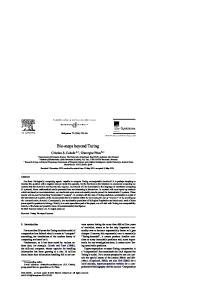
CHAPTER 7. TURING MACHINES b a b a input tape

reject indicator

finite control unit

a c

$ $

...

bidirectional read/write head

accept indicator

Figure 7.1: Conceptually, a Turing machine is very similar to a finite automaton; the main differences are that it can move the head both left and right, and that it can write on as well as read from the tape. The machine can also access as much of the tape as it wishes, using the initially blank-filled tape beyond the input string as scratch space. Here, “$” denotes the blank symbol, which will be our usual convention.

Theorem 28 (Church-Turing Thesis) Any effective procedure is also Turing computable. This statement is known as a thesis rather than a theorem, because is cannot actually be proven due to the informal status of the notion of effective computability.1 This thesis states that Turing machines, an abstract notion of a computer devised by Alan Turing in 1936 [24], can compute anything that has an effective procedure; in essence, it can compute anything that is computable.2 We next formalize the notion of a Turing machine, and explore some of its properties.

7.1

Formal Definition of Turing Machines

As with the other abstract machines that we’ve studied, the Turing machine can read the symbols of a string, which we imagine to be printed on a “tape” that is semi-infinite (i.e. infinite in one direction, to the right). As with all previous machines, a Turing machine begins with the head over the first cell of the tape and can move its head in discrete steps, one cell at a time. There are four fundamental characteristics that distinguish Turing machines from the other machines we’ve encountered so far are: 1. The head can move in either direction (left or right) at each transition. Thus, the head is bidirectional. 2. The head can both read and overwrite symbols on the tape. Thus, it is a read/write head. 3. The head can move arbitrarily far along the tape; i.e. past the input string. 1 While the Church-Turing thesis cannot be proven, it is falsifiable: If some obviously effective procedure were demonstrated to be beyond the capabilities of a Turing machine, the Church-Turing thesis would thereby be proven false. Thus far, this has not happened. While controversies may still arise as to whether computers can ever solve certain problems, our failure to construct such programs may easily be due to ignorance, or to the fact that such problems are not effectively computable to begin with. Only when the latter two possibilities are ruled out would we have a counterexample to the Church-Turing thesis. Until then, the Church-Turing thesis stands as a very plausible theorem. 2 This capability is not peculiar to Turing machines alone. In fact, there are many abstract models of computation that are exactly equivalent to Turing machines in terms of what they can compute. These include recursive functions, Markov algorithms, random access machines, lambda calculus, and unrestricted grammars.

7.1. FORMAL DEFINITION OF TURING MACHINES

93

Turing Machines Initialization • The state of the machine is set to the initial state, q0 . • The input string is written on the tape starting in the first cell of the tape, and all other cells have blank symbols. • The read/write head is positioned over the first cell of the tape, which is the first symbol of the input string. Transitions determined by • The current state. • The symbol under the read/write head. Effect of each transition • The control unit advances to one of a finite number of states. • The symbol under the read/write head is overwritten. • The read/write head moves exactly one cell to the right or to the left, or remains stationary.3 Halts when • An undefined transition is encountered. The machine then “accepts” if the current state is an accept state, and “rejects” otherwise. (As accept states are allowed to have no outgoing transitions, entering such a state is guaranteed to halt the machine and accept.)

Figure 7.2: The semantics of Turing machines. To completely specify how the machine operates we must define how the computation starts, how it proceeds, and how it terminates. These are outlined above.

4. Computation stops if and only if an undefined transition is encountered, and this can happen at at any time, regardless of where the read/write head is positioned. These characteristics make the Turing machine extraordinarily powerful; in fact, no abstract machine or procedure with a mathematically precise definition has ever been shown to be more powerful. That is, according to present-day knowledge (and the Church-Turing thesis), a Turing machine can compute anything that is effectively computable. Figure 7.1 depicts a conceptual Turing machine, with its infinite tape and bidirectional read/write head. To be precise about the behavior of such a machine we must unambiguously specify how the machine starts, how its computation proceeds in discrete steps, and how computation terminates; these behaviors are summarized in Figure 7.2.

94

CHAPTER 7. TURING MACHINES

Formal Definition of a Turing Machine as a 6-tuple: (Σ, Γ, Q, q0 , A, ∆) Symbol

Name

Description

Σ

Input alphabet

Finite non-empty set for encoding input strings.

Γ

Tape alphabet

Finite superset of Σ, used during computation.

Q

State set

Finite non-empty set of state labels.

q0

Initial state

The machine starts in this special state of Q.

A

Accept states

The machine halts (and accepts) when it enters one of these states.

∆

Transition relation

Finite subset of ((Q − A) × Γ) × (Q × Γ × {L, S, R})

Figure 7.3:

A Turing machine can be formally specified as a 6-tuple, with five of elements carrying the same meaning as those of a DFA; the element Γ is new, and the transition relation ∆ is different, since the machine can write on the tape and also move the head to the left. The transition relation is not allowed to have any transitions that leave an accept state, which implies that the machine will always halt (and accept) when such as state is entered.

Formally, a Turing machine may be specified as a 6-tuple (Σ, Γ, Q, q0 , A, ∆), where the transition relation ∆ consists of tuples that determines the new state, the symbol to be written, and the motion of the read/write head. The meanings of each of these symbols is outlined in Figure 7.3. The string that is written on the tape before computation begins must be a string in Σ∗ . Once computation begins, the machine can read or write any symbol in Γ, which typically contains additional symbols that act as markers and simplify the operation of the machine.4 We require Σ ⊆ Γ, b ∈ Γ − Σ. Thus, the input string cannot contain embedded blank symbols; this restriction ensures that the machine can always unambiguously find the end of the input string. Turing machines can be used to recognize languages by accepting or rejecting strings that are written on its tape, just as we have done for all previous machines. When the machine enters its accept state, it halts and signals that the string has been accepted. If the machine encounters an undefined transition and it is not in an accept state, it halts and signals that the string has been rejected. We explicitly prohibit transitions out of an accept state, which guarantees that the machine will always halt when such a state is encountered. Technically, there is no need to have multiple accept states in a Turing machine; all transitions into an accept state are equivalent and can be routed to a single such state with no change in the machine’s behavior. For this reason, Turing machines are often defined to have precisely one “halt” state.5 We allow a set of accept states, however, simply to keep the definition close to those of previous machines. Since Turing machine computation does no stop automatically when the end of the string is reached, the machine need only signal acceptance or halt when it is “ready” to do so. That is, the machine can stop at any time, including before the entire input string is read, or long past the end of the string, or even not at all. This is a crucial difference with previous machines and makes the study of Turing machines a vastly richer subject. 4 Although

only two symbols suffice, it is far more convenient to allow arbitrarily large input and tape alphabets. choose to define Turing machines to signal acceptance or rejection by writing “yes” or “no” (in some appropriate encoding) on the tape. As this makes the machines somewhat more complex, we have opted here to adopt the more expedient mechanism of signaling via an “accept” state, which doubles as a “halt” state. 5 Some

7.1. FORMAL DEFINITION OF TURING MACHINES

95

If M is a Turing machine and w ∈ Σ∗ is a string in its input alphabet, we shall use the notation SM (w) to denote the set of accept states reachable by M as a result of reading string w; this may be any subset of A, including the empty set. As usual, if SM (w) ∩ A is nonempty, we will say that the machine accepts or recognizes the string w. The set of all recognized strings constitutes a language associated with M . More precisely, we define L(M ) = {w ∈ Σ∗ | SM (w) ∩ A 6= ∅} def

(7.1)

to be the language accepted (or recognized) by M . In keeping with previous terminology, we will call a language Turing-acceptable if and only if there exists some Turing machine that accepts it. However, unlike the other machines that we’ve encountered, this does not completely specify what happens with strings that are not accepted; in particular, it is possible that the machine rejects the string, or that it simply never halts. This will lead to the notion of a Turing-decidable language, which we define below.

7.1.1

State Diagrams

As with NFAs, DFAs, and PDAs, Turing machines admit a convenient representation in terms of a state diagram. We retain all of the same conventions as with DFAs regarding the representation of states, transitions, and designating the start state and accept states. The only difference is how we label the arrows of the diagram. In the state diagram of a Turing machine, the transition ((p, a), (q, b, h)) is denoted by an arrow from state p to state q bearing the label a/b; h, where h ∈ {L, S, R}. This transition means that when the machine is in state p and the read/write head is over the symbol a, then the machine is put into state q, the symbol a is replaced by symbol b, and the read/write head moves in direction h by one cell (i.e. to the right if h = R, to the left if h = L, and left where it is if h = S). Figures 7.5 and 7.6 are two examples of Turing machine state diagrams.

7.1.2

Configurations and the Yields Relation

Unlike DFAs, where the portion of the tape that has already been read can no longer influence the operation of the machine, a Turing machine can revisit any portion of its tape any number of times. Consequently, to take an instantaneous snapshot of a given Turing machine at any point in time during its computation, we must record three things: the current state, the contents of the entire tape, and the position of the read/write head. A particularly convenient way to encode this information is by partitioning the contents of the tape into two strings, a “left” and a “right” portion, relative to the position of the head. Thus, we define a Turing machine configuration to be an element of the set Γ∗ × Q × Γ+ . If (u, q, v) is a configuration, u is the content of the tape to the left of the head (which will be the empty string when the head is at the left-most cell of the tape), q is the current state, and v is the content of the tape from the head position to the last non-blank symbol, if that symbol occurs at or to the right of the head. If the tape is blank from the head position on, v consists of a single blank symbol. We can now define the yields in one step binary relation, ` , on the set of configurations. As shown in Figure 7.4, there are three cases to consider, corresponding to moving the read/write head left,

96

CHAPTER 7. TURING MACHINES

right, or not at all. If the transition requires the head to move left when it is already in the left-most cell of the tape, the head is not moved; that is, it is treated exactly as if the transition had specified that the head be stationary. As with previous yields relations, we define the reflexive transitive ∗

closure of the relation, ` , in the usual way. The result is the yields in zero or more steps relation for Turing machines. Using this relation, we can provide an equivalent definition of the language accepted by a Turing machine M = (Σ, Γ, Q, q0 , A, ∆): ½ ¾ ∗ def ∗ ∗ L(M ) = w ∈ Σ | ∃u, v ∈ Γ , (ε, q0 , w) ` (u, qa , v) for some qa ∈ A , (7.2) In the case of nondeterminism, there may be many possible ways to continue the computation from a given configuration. The above definition still holds in such a case, however, as the only requirement is that some sequence of nondeterministic choices (i.e. some branch of the computation) causes the machine to enter an accept state. This interpretation is consistent with the notion of accepting strings in the previous machines that we have studied.

7.2

The Repertoire of Turing machines

Turing machines have a larger repertoire of behaviors than the simpler machines we’ve discussed because they can alter the contents of their tapes and they may fail to terminate. However, every computation of a Turing machine falls into one of three categories: 1. Accept a language 2. Decide a language 3. Enumerate a language 4. Compute a function We say that a Turing machine accepts a language L if for any string w ∈ L it will eventually enter the accept state, and therefore halt. However, for any string w 6∈ L the machine may either reject or loop (i.e. run forever). We say that a Turing machine decides a language L if for any string w ∈ L it will eventually enter an accept state, and for any string w 6∈ L it will reject. Consequently, a machine that decides a language will never loop. We say that a language is Turing-acceptable if there exists a Turing machine that accepts it. We say that a language is Turing-decidable if there exists a Turing machine that decides it. All Turingdecidable languages are also Turing-acceptable. The most fundamental example of a language that is Turing-acceptable but not Turing-decidable is LH = { hM, wi | M is a Turing machine, and M halts on input w } , where hM, wi means an encoding of the machine M and its input string w as a string over some (generally different) alphabet Σ.6 That is, LH consists of strings that each encode a Turing machine 6 Observe that any Turing machine M can be specified by its 6-tuple representation which, in turn, can be encoded in any alphabet with two or more symbols, regarless of how many symbols M has in its alphabet. For example, each symbol could be represented by a unique unary or binary encoding.

7.2. THE REPERTOIRE OF TURING MACHINES

((p, b), (q, c, R)) ∈ ∆ ((p, b), (q, c, S)) ∈ ∆ ((p, b), (q, c, L)) ∈ ∆

=⇒ =⇒ =⇒

97

(ua, p, bv) ` (uac, q, v) (ua, p, bv) ` (ua, q, cv) (ua, p, bv) ` (u, q, acv)

Figure 7.4: The yields relation for Turing machines has three cases, corresponding to the three possible head motions. Here, u and v are arbitrary strings, and b and c are symbols; representing the left and right strings by ua and bv, respectively, simplifies the description of the yields relation. In the case where h = L and the head is at the left end of the tape, the transition is handled as though h = S.

a/a;R b/b;R q1 a/$;R q0

$/$;L

$/$;R

b/$;R q2

$/$;S

q3 a/$;L

q5

a/a;L b/b;L

qa

b/$;L $/$;L

q4

$/$;S

a/a;R b/b;R $/$;S Figure 7.5: A deterministic Turing machine decides the language of palindromes over the alphabet Σ = {a, b}. The strategy is to match left and right symbols, overwriting them with blank symbols, and working toward the center of the string. The machine recognizes palindromes of both even and odd length.

and an input string to run it on. Specifically, it encodes only those Turing machines and inputs for which the machine ultimately halts (accepts or rejects). This language encapsulates the halting problem. A simple diagonalization argument can be used to show that LH is undecidable; that is, that there is no Turing machine that recognizes this language and is guaranteed to always halt. A Turing machine can also be used to compute a function from strings to strings, since it can leave a different string on the tape than the one it began with. Thus, we say a Turing machine computes a function f : Σ∗ → Γ∗ if, when run on string w ∈ Σ∗ , it eventually halts with the string v = f (u) written on the tape starting in the first cell. We’ll need to be careful about cases in which the machine fails to halt, however, as we shall see later.

98

CHAPTER 7. TURING MACHINES

/1;S 1/1;R 0/0;R 0/0;R

q0

q1

1/0;L / ;L

q2

0/1;S

qa

1/1;R / ;R

q3

/0;S 0/1;R

q4 0/0;R

Figure 7.6: A deterministic Turing machine that “adds one” to its input string. That is, if the input is a string in {0, 1}∗ that encodes a number in binary notation, what is left on the tape when the machine halts is the binary encoding of that number plus one. Note that the head position at the end is immaterial here.

7.3

Extended Turing Machines

Although our definition of a Turing is fairly close to that originally proposed by Alan Turing in 1936 [24], it is reasonable to ask whether different constructs might have lead to a broader definition of computability. As it happens, the standard Turing machine definition is extremely robust; indeed, it has proven capable of simulating every other machine that has ever been conceived. In this section we will show that this is so for two important extensions to the standard Turing machine: those with bi-infinite tapes, and those with multiple tapes.

7.3.1

Bi-Infinite Tapes

What would happen if we allowed the Turing machine to have a bi-infinite tape; that is, a tape that is infinite in both directions (left and right)? By definition, the computation of such a machine begins with the read/write head over the first symbol of the input string (or anywhere if the input string is empty). Theorem 29 A Turing machine with a bi-infinite tape is equivalent to a standard Turing machine (in terms of computability). Proof: (Sketch) All we need to show is that, given such a machine M with a bi-infinite tape, its behavior can be simulated exactly by a Turing machine with only a semi-infinite tape. To do this, we start with the machine M and modify it slightly so that it does not ever attempt to move the head off the left end of the tape, yet it manages to carry out the very same computation as the original machine. This new machine will then be able to operate in exactly the same way as the machine with the semi-infinite tape.

7.3. EXTENDED TURING MACHINES

...

$

bi-infinite tape $ $ a b a

finite control unit

a c

b $

bidirectional read/write head

99 $ $

$ $

$ $ $ $ "scratch" tape

...

a b

z

a $ $ $ "scratch" tape

...

a c

...

x

... b a b a input tape finite control unit

b $

multiple bidirectional read/write heads

Figure 7.7: There are many variations that one can envision for the basic Turing machine. Two obvious modifications that one could make are (left) to allow the tape to be “bi-infinite” (i.e. infinite in both directions), and (right) to allow multiple tapes. Both of these modifications can be simulated by a standard Turing machine.

There are many strategies that could be employed to do this. The easiest way is to have the machine start by replacing the first symbol on the tape (which is a blank) by a new marker. Let’s call that symbol “#”. We also add to the machine’s transition relation and states so that whenever the “#” symbol is encountered, the machine moves the contents of the tape to the right by one, inserts a blank symbol immediately to the right of “#”, and continues the computation with the read/write head over that new blank symbol. This modification allows the machine to seemingly “grow” the tape to the left (by pushing the tape contents to the right) as far as it needs to without ever changing what is ultimately computed. ¤

7.3.2

Multiple Tapes

As quickly becomes evident when attempting to create Turing machines that carry out various computations, a great deal of thought and effort usually goes into moving the head around, copying results from one part of the tape to another, and leaving markers for various purposes. All of this could be simplified greatly if the Turing machine had multiple tapes, each with its own bidirectional read/write head. So, suppose we had defined a Turing machine to have k tapes (for some integer k), and a transition relation that depends on the current state as well as the symbols under all of the read/write heads, and specifies which direction to move each head as well as which symbol to write on each tape. One tape would be designated as the input tape (where the input string w is written, as before), and the other k − 1 tapes could be used for arbitrary computations. Such a machine would surely be easier to “program,” but would it change the class of Turing-acceptable or Turing-decidable languages? The answer is easily seen to be “no.” Theorem 30 A k-tape Turing machine is equivalent to a standard 1-tape Turing machine (in terms of computability). That is, the class of Turing-acceptable and Turing-decidable languages is exactly

100

CHAPTER 7. TURING MACHINES

the same for all k-tape machines, where k ≥ 1. Proof: (Sketch) Since the k-tape machine is clearly as powerful as a 1-tape machine, we need only show that a 1-tape machine can (in principle) accomplish anything that a k-tape machine can, for any fixed k ≥ 2. Again, there are a number of different approaches that we could take. Perhaps the easiest to visualize is partitioning the tape into k sectors, each representing one “virtual” tape. Within each virtual tape, a marker would be kept to indicate the location of the virtual head (and the symbol beneath it). When any of the first k − 1 tapes reaches the end of the sector, the contents of the tape from that point down would be moved down before the computation is be resumed. Thus, each virtual tape would behave as though it is semi-infinite. The machine would search for the virtual head within each sector and advance the computation one step, then start again with the first virtual tape. This construction is somewhat cumbersome, and would certainly lead to very inefficient machines, but it should be clear that exactly the same computation could eventually be carried out by the 1-tape machine as performed by the k-tape machine. This is all we need to show. ¤

7.4

Nondeterminism

As with the previous machines that we have studied, Turing machines may be be constructed with one or more ambiguous transitions, which makes them nondeterministic. We will use the abbreviations DTM and NTM for deterministic and nondeterministic Turing machines, respectively, when it is important to make the distinction. A Turing machine M = (Σ, Γ, Q, q0 , A, ∆) is nondeterministic if and only if there are one or more ambiguous transitions, which is to say ((p, a), (q, b, d)) ∈ ∆ ∧ ((p, a), (q 0 , b0 , d0 )) ∈ ∆,

(7.3)

for some p ∈ Q and some a ∈ Γ, where (q, b, d) 6= (q 0 , b0 , d0 ); that is, where at least one of the components in the 3-tuples is differs between the two transitions. When this is the case, then the machine must make a nondeterministic choice among the alternatives whenever it is in state p with the symbol a under the read/write head. As with DFAs and NFAs, we will see that DTMs and NTMs are equivalent in terms of languages that they recognize (for both accepting and deciding). However, there is an apparent difference in power between the two machines when we consider the number of steps that they require to perform these computations, as we shall see later. Theorem 31 In terms of which languages can be accepted or decided, nondeterministic Turing machines are equivalent to deterministic Turing machines. Proof: (Sketch) A multi-tape deterministic Turing machine can simulate a nondeterministic Turing machine by maintaining a “queue” of possible configurations. That is, whenever the nondeterministic machine would encounter a nondeterministic branch, the simulator would copy multiple resulting configurations to the queue. Each configuration is “run” exactly one step before being copied back to the end of the queue. If any configuration ever reaches an accept state, the simulator accepts.

7.5. UNIVERSAL TURING MACHINES

101

This process is referred to as dovetailing. ¤ A question naturally arises as to what it means for a nondeterministic machine to loop. Does it mean that the machine loops for all branches the computation could follow, or that it loops for at least one branch that the computation could follow? The definition that makes the most sense becomes apparent when we consider what it means for a nondeterministic machine to accept a string; here it is only required that one possible branch of the computation reach an accept state, regardless of what happens on the other possible branches. Thus, if the NTM M has even one branch that reaches an accept state when run on w, then the machine is clearly considered to halt on w. Moreover, its deterministic equivalent, as described above, will eventually halt on such a w. Similarly, if all branches of the computation reject w, then the machine is considered to halt, and its deterministic equivalent will halt on w. The problem arises when no branch accepts w, and at least one branch loops on w. It is precisely this case in which the deterministic equivalent will loop, and therefore the nondeterministic machine is also said to loop. We summarize this in the following definition. Definition 22 A nondeterministic Turing machine M is said to loop on input string w if and only if there is no sequence of nondeterministic choices that will cause the machine to enter an accept state (thus accepting the string), and at least one sequence of nondeterministic choices will cause the machine to loop.

7.5

Universal Turing Machines

Alan Turing also noted that his abstract machine was capable of being “programmed.” That is, one could construct a special Turing machine whose job is to interpret and run (or simulate) any other Turing machine being run on any input; we call such a machine a universal Turing machine. One can think of a universal Turing machine as being a precursor to modern-day programmable machines that can carry out virtually any task merely by changing its “software.”7 We state this as a theorem. Theorem 32 There exists a Turing machine, U , that can simulate the behavior of any given Turing machine, M , on any given input string, w, provided that M and w are properly encoded using the input alphabet of the machine U . We will denote the encoding of M and w together using some fixed alphabet as hM, wi. This is a minor complication which arises from the fact that different Turing machines can be defined with different alphabets. The universal machine is to handle any possible Turing machine as input, even those with larger alphabets, thus it is necessary to express them entirely in the input alphabet of the fixed universal machine. The notation hM, wi also implies that the strings encoding M and w are unambiguously separated, either by a special marker or some sequence of symbols, so that the machine that is reading the encoding can determine where one ends and the other begins. Proof: (Sketch) To be supplied. 7 This

is in contrast to the earliest electronic computers, which needed to be “rewired” for each task.

102

7.6

CHAPTER 7. TURING MACHINES

Algorithms and Deterministic Turing Machines

Let M be a deterministic Turing machine and let CompM (w) denote the content of the tape beginning at the current head position up to but not including the next occurrence of the blank symbol. If the machine never halts, we shall denote the value of CompM (w) by ↑. That is,    ↑ if M (w) = {↑} def 5 if M (w) = {5} CompM (w) = ∗   u if (ε, q , w) ` (v, qa , u) for some qa ∈ A 0

(7.4)

For the purposes of computing functions, there is be no reason to halt by encountering an undefined transition. We have specifically constrained M to be deterministic so that we can speak of the single value that M produces upon reading w. If our intention had been to capture the notion of multi-valued functions, we could have done so simply by allowing M to be nondeterministic.

Definition 23 Let f : Σ∗1 → Σ∗2 be a (total) function. If there exists a deterministic Turing machine M such that CompM (w) = f (w) for all w ∈ Σ∗1 , then we say that f is recursive. In this case we also say that M computes f , and that there exists an algorithm for computing f .

Observe that, according to this definition, an algorithm always terminates. This is a consequence of f being a total function, as this implies that M must provide a value (and therefore halt) for every input string. It is sometimes useful to relax this restriction, however, which leads to a natural generalization.

Definition 24 Let f : Σ∗1 → Σ∗2 be a partial function, and let us write f (w) = ↑ for all w on which f is undefined. If there exists a deterministic Turing machine M such that CompM (w) = f (w) for all w ∈ Σ∗1 , then we say that f is partial recursive. In this case we also say that M computes f , and that there exists a partial algorithm for computing f .8

Thus, for all w on which f is undefined, the machine M loops (i.e. never halts). The terms recursive and partial recursive were borrowed from the theory of recursive functions. Fortunately, the terms mean exactly the same thing in both contexts. That is, a recursive function is one that is total and can be expressed in terms of unbounded minimization and primitive recursive functions and operators, and it is also a total function that can be computed by a deterministic Turing machine. The term “partial recursive” is similarly consistent. For historical reasons, the terminology has become intertwined, so one commonly encounters terms coined for the theory of recursive functions when dealing with Turing machines, and vise versa. The somewhat surprising fact that these different abstractions lead to precisely the same sets of languages made it permissible to freely interchange terminology.

7.7. TURING-ENUMERABLE LANGUAGES

103 /a;R

#/a;R

q0

/#;R

q1

/#;S

q2

q0

(a)

/#;R

q1

/#;S

q2

(b)

Figure 7.8: Two different Turing machines that enumerate the language a∗ . Rhe deterministic machine (a) repeatedly appends a’s, and moves the # marker down. The nondeterministic machine (b) writes a string of a’s of indeterminate length, then halts.

7.7

Turing-Enumerable Languages

Another task that a Turing machine can perform is to enumerate a collection of strings, in analogy with a program that appends a sequence of strings to a file or sends the strings to a device such as a printer. Rather than extending the notion of a Turing machine by affixing some kind of output device, we can simply adopt a convenient convention by which a standard Turing machine can be said to generate a list of strings. So long as such a “list” could, in principle, be captured in some way, perhaps by being sent off to another machine, it will suffice for our purposes. Toward this end, we define the Turing machine output operator as follows ∗ Γ Out# M :Σ → 2

(7.5)

that depends on a given Turing machine M and a special marker # in its tape alphabet Γ. This operator associates each input string w ∈ Σ∗ with a set of strings over the alphabet Γ−{#} according to the following rule: ½ ¾ ∗ def # ∗ ∗ OutM (w) = u ∈ Σ | (ε, q0 , w) ` (v1 #u, q, #v2 ), q ∈ Q, v1 , v2 ∈ Γ . (7.6) That is, when the machine is run on the string w, every string that at some time appears on the tape, flanked by # symbols, with the head positioned over the right # symbol, is in the set. The machine may halt or loop, and it may generate either a finite or infinite set of strings with or without repetition. In terms of the printer analogy, think of the machine doing the following: Each time the head is positioned over a # symbol, either by moving the head onto an existing symbol or by overwriting the current symbol and leaving the head fixed, then the content of the tape is scanned to the left until another # symbol is found. The string consisting of all the intervening symbols is printed. If there is no # symbol to the left, the string is not printed. If the language L is infinite, then the enumerator will never halt. If the language is finite, the enumerator may or may not halt. Observe that the definition does not specify whether the strings are to remain on the tape; consequently, whether they are eventually overwritten or not is immaterial. Figure 7.8 shows two different machines that enumerate the language a∗ , with and without 8 The terminology “partial algorithm” is not yet widely adopted. However, since the word “algorithm” is commonly reserved for computations that always halt, it is useful to have some way to refer to those that may possibly loop; “partial algorithm” seems to be an obvious choice.

104

CHAPTER 7. TURING MACHINES

nondeterminism. Notice that in Figure 7.8b it is essential that the transition from state q1 to q2 leave the head stationary; otherwise, according to the definition we have given, the machine would enumerate the empty language. We say that M enumerates the language L ⊆ Γ∗ (using marker #) if and only if L = Out# M (ε)

(7.7)

for some # ∈ Γ. Definition 25 We say that a language L is Turing-enumerable if and only if there exists a Turing machine M that enumerates L. That is, when M is run on a blank tape, it eventually writes every string of the language L as the last non-blank string on its tape, beginning at the position of the read/write head. The machine signals the presence of each string by entering a special state, q ∗ , and (generally) keeps going, generating more strings. If the language L is infinite, the machine must be nondeterministic, non-halting, or both.9 As with nearly every definition involving Turing machines, Turing-enumerability could has been defined in numerous other ways, all of them equivalent. For example, we could insist that the machine generate an ever-growing list of strings in the language, all separated by some special marker. See Exercises (10) and (11) for several other definitions. Note that it is only required that M generate each string in L at least once; it is not required that M generate it exactly once. It is also required that every time M enters state q ∗ , the string to the right of the head is in L. As it happens, we have encountered the set of r.e. languages before, but under a different name. Theorem 33 A language is Turing-acceptable if and only if it is Turing-enumerable. Proof: (=⇒) Suppose that L is Turing acceptable and that Ma is a Turing machine that accepts it; that is, L = L(Ma ). Then we can construct another Turing machine Me that enumerates L as follows. The machine Me nondeterministically writes a string w to the tape, then behaves exactly like Ma with w as its input. If Ma would accept, then Me writes w at the end of its tape, and enters state q ∗ , otherwise it does not enter state q ∗ . (⇐=) Suppose that L is r.e. and that Me is a Turing machine that enumerates it, with q ∗ as the special state. Then we can easily construct a machine Ma that accepts L as follows. The machine Ma behaves very much like Me , generating all strings in L, except that whenever it would enter the state q ∗ it compares the original input string with the string at the end of the tape. If they match, the machine enters the accept state. If not, the machine continues to generate strings in L. ¤

Theorem 34 A language L is decidable if and only if both L and L are recursively enumerable. 9 If the language L is infinite, and the machine that enumerates it simply nondeterministically chooses any one of the strings of the language to write on its tape, then halts, its deterministic equivalent will never halt.

7.8. EXERCISES

105

Proof: (=⇒) If a Turing machine M decides L (and therefore accepts L), then we can easily modify it to decide (and therefore accept) L; we simply remove all transitions to the accept state, and fill in all transitions that were initially missing with transitions to the accept state. (⇐=) If M and M are two Turing machines that accept L and L, respectively, then we can build a new Turing machine MD that decides L as follows: We construct MD as a multi-tape Turing machine that simulates the actions of both M and M on a given string w, perhaps on separate tapes, by alternating from one to the other. One of these two machines is guaranteed to enter an accept state, thereby accepting the string, since w is either in L or it is in L. If M accepts w, then MD accepts w. If M accepts w, then MD rejects w. Either way, the machine MD will halt, and it will recognize the same language as M . Therefore, L is decidable. ¤

Theorem 35 A language is Turing-enumerable if and only if it is recursively enumerable. Proof: (To be supplied.) ¤ Because of theorem 35 and theorem 33 the term recursively enumerable is a synonym for both Turingenumerable and Turing-acceptable. In fact, the term recursively enumerable, and its abbreviation “r.e.”, are much more common in the computer science literature than either Turing-enumerable or Turing-acceptable. Henceforth, we will use the term recursively enumerable, or the abbreviation r.e. in lieu of both.

7.8

Exercises

1. Provide a state © diagram andªa brief description of a deterministic Turing machine that decides the language an b2n | n ≥ 0 . 2. Provide a state diagram and a brief description of a deterministic Turing machine that computes the function f : Σ∗ → Σ∗ given by f (w) = c|w| #wR , where Σ = {a, b} and both “c” and “#” are additional symbols in Γ. That is, the output string should be a string of c’s with the same length as the original string, followed by a “#” symbol, followed by the reverse of the original string. 3. Let Σ = {0, 1}. Construct a deterministic Turing machine that computes the function f : Σ∗ → Σ∗ such that f (hni) = h2n + 1i for all n ∈ N, where hni means the encoding of the integer n as a binary number; that is, as a string in Σ∗ . The most significant digit should be in cell number 2 of the tape, so that the number appears on the tape as one would normally write it. the state diagram and a brief description of a Turing machine that decides the language 4. Give © n 2n ª a b cn | n ≥ 0 . 5. Describe how to construct a Turing machine that decides the language {an | n is a power of 2 }, and give a complete state diagram of the machine.

106

CHAPTER 7. TURING MACHINES

6. Let Σ = {0, 1}. Construct a deterministic Turing machine that computes the function f : Σ∗ → Σ∗ such that f (hni) = h3ni for all n ∈ N, where hni means the encoding of the integer n as a binary number; that is, as a string in Σ∗ . The most significant digit should be in cell number 2 of the tape, so that the number appears on the tape as one would normally write it. (a) Carefully describe the idea behind your machine. (b) Draw a complete state diagram of the machine. 7. Let Σ = {0, 1}. Construct a deterministic Turing machine that accepts the language L = {w ∈ Σ∗ | Collatz(n) is finite, where w = hni }, where again hni means the encoding of n as a binary number. Here, Collatz(n) means the Collatz sequence generated beginning with n. Please refer to homework #3 for the definition of the Collatz sequence. (a) Carefully describe the idea behind your machine. (b) Draw a complete state diagram of the machine. (Since this machine builds upon your solution to the previous problem, you need not copy your entire state diagram. You may merely indicate how it would be incorporated into the new state diagram.) 8. Construct a deterministic Turing machine that computes the function f (w) = wR , where the input alphabet is Σ = {a, b}. 9. Construct a non-deterministic Turing machine that accepts the language unary-composite, which consists of the strings ak , where k is not prime. Hint: non-deterministically overwrite the first m symbols in the input string, where m < k, then produce copies of this new string until the original string is completely overwritten. If there is no “remainder,” then enter an accept state. Otherwise, reject. 10. Show that the following definition of Turing-enumerability is equivalent to the one given earlier. A language is Turing-enumerable if there exists a Turing machine that can write sequence of strings #u1 #u2 #u3 # · · · ., where each ui is in the language. Once the # is written, nothing on the tape to its left is ever changed. Moreover, for any w ∈ L, the sequence will eventually contain w, flanked by # symbols, and will never be disturbed by the machine. 11. Show that we could have defined Turing-enumerability as follows: there exists a Turing machine ∗

M such that for some special state q ∗ ∈ Q, w ∈ L if and only if (ε, q0 , $) ` (u, q ∗ , w) where u is any string over the tape alphabet. That is, we use entering of a specially-designated signalling state to indicate when a new string has been written. 12. Construct a nondeterministic Turing machine M that does the following: given an input ∗ ∗ string w ∈ {a, b} , M “guesses” a string in {0, 1} of the same length; that is, the machine non-deterministically writes a string of length |w| (overwriting the original string) consisting of 1’s and 0’s, such that any such string might be written. 13. Consider the following languages: (a) (b) (c) (d)

L1 L2 L3 L4

= {hM i | M enters each of its states at least once given input ε} = {hM, wi | M halts after |w| + 100 steps given input w} = {hM i | L(M ) is finite} = {hM, wi | M never moves its head to the left given input w}

Determine whether each of these languages is decidable or undecidable. Prove your answers.