PHYSICAL REVIEW E 72, 036133 共2005兲
Tuning clustering in random networks with arbitrary degree distributions M. Ángeles Serrano1 and Marián Boguñá2
1
School of Informatics, Indiana University, Eigenmann Hall, 1900 East Tenth Street, Bloomington, Indiana 47406, USA 2 Departament de Física Fonamental, Universitat de Barcelona, Martí i Franquès 1, 08028 Barcelona, Spain 共Received 22 July 2005; published 30 September 2005兲 We present a generator of random networks where both the degree-dependent clustering coefficient and the degree distribution are tunable. Following the same philosophy as in the configuration model, the degree distribution and the clustering coefficient for each class of nodes of degree k are fixed ad hoc and a priori. The algorithm generates corresponding topologies by applying first a closure of triangles and second the classical closure of remaining free stubs. The procedure unveils an universal relation among clustering and degreedegree correlations for all networks, where the level of assortativity establishes an upper limit to the level of clustering. Maximum assortativity ensures no restriction on the decay of the clustering coefficient whereas disassortativity sets a stronger constraint on its behavior. Correlation measures in real networks are seen to observe this structural bound. DOI: 10.1103/PhysRevE.72.036133
PACS number共s兲: 89.75.Hc, 87.23.Ge, 05.70.Ln
I. INTRODUCTION
Models in complex network science aim to reproduce some common empirical statistical features observed across many different real systems, from the Internet to society 关1–3兴. Many of those models are able to recreate prominent recurrent attributes, such as the small-world property and scale-free degree distributions with characteristic exponents between 2 and 3 as measured for networks in the real world. Other characteristics, such as the presence, the shape, and the intensity of correlations, are also unavoidable in models intending to help us to understand how these complex systems self-organize and evolve. The first reference to correlations in networks appearing in the literature is the clustering coefficient 关4兴, which refers to correlations among three vertices. The clustering is a measure of transitivity which quantifies the likelihood that two neighbors of a vertex are neighbors themselves. Then, it is a measure of the number of triangles present in a graph. In addition to the empirical evidence that the vast majority of real networks display a high density of triangles, the concept of clustering is also relevant due to the fact that triangles are—together with edges—the most common building blocks taking part in more complex but elementary recurring subgraphs, the so-called motifs 关5兴. It has been argued that network large-scale topological organization is closely related to the network’s local motif structure 关6兴 so that these subgraphs could be related to the functionality of the network and can be fundamental in determining its community structure 关7,8兴. All these mean that a correct quantification and modeling of the clustering properties of networks is a matter of great importance. However, most modeling efforts beyond the degree distribution have focused on the reproduction of twopoint correlation patterns, typified by the average nearestneighbor degree 关9兴, so that clustering is just obtained as a by-product. In most synthetic networks, it vanishes in the thermodynamic limit, but as to many other respects, scalefree networks with a divergent second moment stand as a special case. The decay of their clustering with the increase 1539-3755/2005/72共3兲/036133共8兲/$23.00
of the network size is so slow that relatively large networks with an appreciable high cohesiveness can be obtained 关10兴. Nevertheless, it remains an indirect effect and no control over its intensity or shape is practicable. Therefore, an independent modeling of clustering is required and a few growing linear preferential attachment mechanisms have been suggested 关11–13兴. One of the proposed models 关11兴 reproduces a large clustering coefficient by adding nodes which connect to the two extremities of a randomly chosen network edge, thus forming a triangle. The resulting network has the power-law degree distribution of the Barabási-Albert model P共k兲 ⬃ k−3, with 具k典 = 4, and since each new vertex induces the creation of at least one triangle, the model generate networks with a finite clustering coefficient. A generalization of this model 关13兴 which allows one to tune the average degree to 具k典 = 2m, with m an even integer, considers new nodes connected to the ends of m / 2 randomly selected edges. Two vertices and three vertices correlations can be calculated analytically through a rate equation formalism. The clustering spectrum is here finite in the infinite-size limit and scales as k−1. A different approach is able to generate networks with a given degree distribution and a fixed scalar clustering coefficient, measured as the frequency of triadic closure 关14兴. Those models do not allow much freedom in the form of the resulting clustering coefficient, neither in the ensuing degree distribution, so that, although a valuable first approach, they constitute a timid attempt as clustering generators. In this paper, we make headway by introducing a generator of random networks where both the degree-dependent clustering coefficient and the degree distribution are tunable. After a brief review of several clustering measures in Sec. II, the algorithm is presented in Sec. III. In Sec. IV, we check the validity of the algorithm using numerical simulations. Section V is devoted to the theoretical explanation of the constraints that degree-degree correlations impose in the clustering. We find that assortativity allows higher levels of clustering, whereas disassortativity imposes tighter bounds. As a particular case, we analyze this effect for the class of scale-free networks. We end the section by examining some
036133-1
©2005 The American Physical Society
PHYSICAL REVIEW E 72, 036133 共2005兲
M. ÁNGELES SERRANO AND M. BOGUÑÁ
empirical networks, finding a good agreement with our calculations. Finally, conclusions are drawn in Sec. VI.
In the case of uncorrelated networks, ¯c共k兲 is independent of k. Furthermore, all the measures collapse and reduce to C 关18–20兴:
II. MEASURES OF CLUSTERING
Several alternative definitions have been proposed over time to quantify clustering in networks. The simplest measure is defined as 关15,16兴 C⌬ =
3 ⫻ 共number of triangles兲 . 共number of connected triples兲
共1兲
This scalar quantity does not give much information about the local properties of different vertices because it just counts the overall number of triangles regardless of how these triangles are placed among the different vertices of the network. The clustering coefficient, first introduced by Watts and Strogatz 关4兴, provides instead local information and is calculated as ci =
2Ti , ki共ki − 1兲
共2兲
where Ti is the number of triangles passing through vertex i and ki is its degree. The average of the local clustering coefficients over the set of vertices of the network, C, is usually known in the literature as the clustering coefficient. Watts and Strogatz were also the first in pointing out that real networks display a level of clustering typically much larger than in a classical random network of comparable size, Crand = 具k典 / N, with 具k典 the average degree and N the number of nodes in the network. Although C and C⌬ are sometimes taken as equivalent, they may be very different, even though both measures are defined in the interval 关0,1兴. With the definition of ci we have gone to the other extreme of the spectrum—from a global to a purely local perspective—so that we have highly detailed information. One can adopt a compromise between the global property defined by C, or C⌬, and the full local information given by ci by defining an average of ci over the set of vertices of a given degree class 关17兴—that is, ¯c共k兲 =
1 1 ci = 兺 兺 2Ti , Nk i苸⌼共k兲 k共k − 1兲Nk i苸⌼共k兲
共3兲
where Nk is the number of vertices of degree k and ⌼共k兲 is the set of such vertices. The corresponding scalar measure is called the mean clustering coefficient and can be computed on the basis of the degree distribution P共k兲 as ¯c = 兺 P共k兲c ¯ 共k兲,
共4兲
k
which must not be confused with the clustering coefficient C =¯c / 关1 − P共0兲 − P共1兲兴. In fact, we have implicitly assumed that ¯c共k = 0兲 =¯c共k = 1兲 = 0 whereas in the definition of C we only consider an average over the set of vertices with degree k ⬎ 1. This fact explains the difference between both measures.
¯c共k兲 = C⌬ = C =
1 共具k2典 − 具k典兲2 , 具k典3 N
k ⬎ 1.
共5兲
Therefore, a functional dependence of ¯c共k兲 on the degree can be attributed to the presence of correlations. Indeed, it has been observed that ¯c共k兲 exhibits a power-law behavior ¯c共k兲 ⬃ k−␣ 共typically 0 艋 ␣ 艋 1兲 for several real scale-free networks. Hence, the degree dependent clustering coefficient has been proposed as a measure of hierarchical organization and modularity in complex networks 关21兴. Recently, a new local clustering coefficient has been proposed, which filters out the bias that degree-degree correlations can induce on that measure 关22兴 ˜ci =
Ti , i
共6兲
where i is the maximum number of edges that can be drawn among the ki neighbors of vertex i. This new measure does not strongly depend on the vertex degree, remaining constant or decreasing logarithmically with the increase of k when computed for several real networks. III. ALGORITHM
In this paper, we develop and test a new algorithm that, in the same philosophy of the classical configuration model 共CM兲, generates networks with a given degree distribution and a preassigned degree-dependent clustering coefficient ¯c共k兲, as defined in Eq. 共3兲. The CM has been one of the most successful algorithms proposed for network formation 关23,24兴. The relevance of the algorithm relies on its ability to generate random networks with a preassigned degree sequence—taken from a given degree distribution—at the user’s discretion while maximizing the network’s randomness at all other respects. The algorithm became relevant as soon as more real networks were analyzed and proved to strongly deviate from the supposed Poisson degree distribution predicted by the classical model of Erdös and Rényi 关25,26兴. Ever since, the CM has been extensively used as a null model in contraposition to real networks with the same degree distribution. One of the well-known properties of the CM is that clustering vanishes in the limit of very large networks 关see Eq. 共5兲兴 and, thus, it clearly deviates from real networks, for which clustering is always present. In general, a high level of clustering may change the percolation properties of the network, alter its resilience in front of removal of its constituents, or affect the dynamics that takes place on top of them. Since such processes inextricably entangle topology and functionality, it would be very interesting to have at one’s disposal an algorithm that generates clustered networks in a controlled way so that one can check which is the real effect of transitivity on its topological and dynamical properties. With this purpose, we introduce an undirected unweighted static model where the total number of nodes in the network,
036133-2
TUNING CLUSTERING IN RANDOM NETWORKS WITH …
PHYSICAL REVIEW E 72, 036133 共2005兲
N, remains constant, as in the case of the CM. The algorithm comprises three different parts: 共A兲 Assignment of a degree to each node and assignment of a number of triangles to each degree class according to the expected distributions, 共B兲 closure of triangles, and 共C兲 closure of the remaining free stubs. In what follows, we give a detailed description of the algorithm. A. Degree and clustering from expected distributions
共i兲 An a priori degree sequence is chosen according to a given distribution P共k兲, so that each vertex is awarded an a priori number of connections in the form of a certain number of stubs. 共ii兲 An a priori clustering coefficient ¯c共k兲 is also fixed, so that each class of nodes of degree k is assigned an a priori number of triangles.1 Note that the number of triangles is fixed for the whole class and not for the particular vertices of the class. This is a key point of the algorithm because fixing the number of triangles to each single vertex would impose a number of constraints that would make nearly impossible to close the network. 共iii兲 All nodes begin with a number of 0 associated edges and all degree classes begin with a number of 0 associated triangles. B. Triangle formation
First we give some preliminary remarks. Both stubs and edges can be selected to form a triangle. Stubs are half links associated with one node, and edges are entire links associated with two nodes and thus have double probability with respect to stubs to be selected to participate in a triangle. Let us define the set of eligible components 共EC’s兲 as the set of free stubs and edges associated with nodes belonging to degree classes with a number of triangles below its expected value 共unsatisfied classes兲. Stubs and edges of nodes in satisfied classes should not be in the set of EC’s. Edges of nodes which cannot form more triangles 共with only edges as components and neighbors without stubs兲 should not be in the set of EC’s. Stubs and edges of nodes with only one component should not be in the set of EC’s. Notice that the set of EC’s changes dynamically as triangles are formed. The algorithm then proceeds by choosing three different nodes and forming a triangle among them whenever it is possible and it did not exist previously. The selection of the nodes is performed hierarchically as follows. 共i兲 For the first node, a degree class k1 among the ones with an unsatisfied number of expected triangles is chosen
FIG. 1. The two selected components of the first node, marked 1, are edges. The triangle is formed by connecting nodes 2 and 3, whenever they have free stubs.
with a certain probability distribution ⌸共k兲 not necessarily uniform 共the specific form for this function and the motivation to introduce it will be discussed at the end of the section and a theoretical explanation is given in Sec. V兲. Then, the node is selected through a component which is chosen with uniform probability within the subset of eligible components in the class, EC共k1兲. A second different component of the same node is selected. 共ii兲 If the two chosen components are edges and the second and third nodes at the end of the edges still have free stubs, the triangle is formed by merging one free stub of the second node and one free stub of the third node 共see Fig. 1兲. 共iii兲 If one component is a stub and the other an edge, a third node is necessary. First, a new component is selected for the second node at the end of the edge. If it is an edge, the triangle is formed by merging one free stub of the first node and one free stub of the third node. If it is a stub, then a third node is chosen in the same way as the first one under the condition that it has two free stubs. The triangle is then formed by merging these two free stubs with the ones of the first and second nodes 共see Fig. 2兲. 共iv兲 It may happen that the two components of the first node are stubs. Then, a new node is selected in the same way as the first one under the condition of having at least one free stub, and a second component is also chosen for this second
1
The expected number of triangles associated with each class is 1 ¯ 共k兲P共k兲N. For very large degrees, it may happen T共k兲 = 2 k共k − 1兲c that this number is smaller than 1. To overcome this problem, one can determine Tk by allocating a number of triangles, Ti, to each vertex i using, for instance, the binomial distribution B共p , Nmax兲 with p =¯c共ki兲 and Nmax = ki共ki − 1兲 / 2. Then, the number of triangles, Ti, are summed up for each class. Once each class has been assigned a total number of triangles, individual vertices forget the initially ascribed Ti.
FIG. 2. The two selected components of the first node are one edge and one stub. A second component is chosen for the second node. On the left side of the figure, the component is an edge whereas on the right side it is a free stub.
036133-3
PHYSICAL REVIEW E 72, 036133 共2005兲
M. ÁNGELES SERRANO AND M. BOGUÑÁ
FIG. 3. The two selected components of the first node, marked 1, are stubs.
node. If both components of the second node are stubs, a third node with two free stubs is selected and the triangle is closed. If one component of the second node is a stub and another an edge, the node at the end of the edge will be the third node and the triangle is formed linking stubs between the first and the second node and the first and third nodes 共see Fig. 3兲. 共v兲 After each triangle is formed, all dynamic quantities are updated: linked stubs are converted into edges and the corresponding number of new triangles is added to all involved degree classes. It is worth mentioning that not only one more triangle is computed for the classes of the nodes forming the triangle, but the degree classes of simultaneous neighbors of pairs of those nodes may also be affected if those pairs were not previously connected. The set EC is also updated, removing components of nodes in new satisfied classes as well as nodes with only one component or nodes which cannot form more triangles. 共vi兲 This process is repeated until all classes are satisfied or there are no more components in the eligible set. C. Closure of the network
The final step consists in the closure of the network by applying the classical configuration model to the remainder stubs. Pairs of these stubs are selected uniformly at random and the corresponding vertices are connected by an undirected edge. In this way, the algorithm is able to reproduce networks with a given degree distribution P共k兲 and a given clustering coefficient ¯c共k兲, as long as the assortativity—that is, positive degree-degree correlations—is high enough to avoid constraining ¯c共k兲. This is by no means a deficiency of the algorithm but a universal structural constraint imposed by the degree-degree correlation pattern of the network. In general, with the maximum assortativity one can reproduce any desired level of clustering, whereas disassortative networks have instead a bounded clustering coefficient. A theoretical explanation is given in Sec. V. In our algorithm, the level of assortativity is controlled by the probability by which the degree class is chosen previously to the selection of the node. This can be done in a number of different ways. In our case, we tune the assortativity by choosing a proper form for the probability ⌸共k兲. For instance, an uniparametric function modeling different assortativity levels is given by ⌸共k兲 ⬀ Tr共k兲, where Tr共k兲 is the number of triangles remaining to be formed in the degree class k in a given iteration. The value of  typically ranges in
FIG. 4. 共Color online兲 Clustering coefficient for networks generated by the algorithm using a Poisson degree distribution with average degree 具k典 = 4 and expected clustering coefficient ¯c共k兲 = c0共k − 1兲−␣ 共solid lines兲 with ␣ = 1,0.7,0.4, and c0 = 0.5 in all cases. Each curve is an average over three different realizations with a network size of N = 105. The parameter  is equal to 1 for ␣ = 1 and ␣ = 0.7 and  = 0.5 for ␣ = 0.4.
the interval 关0,1兴, generating more assortative networks as  approaches 0. IV. NUMERICAL SIMULATIONS
To check the feasibility and reliability of the algorithm, we have performed extensive numerical simulations, generating networks with different types of degree distributions and different levels of clustering. The chosen forms for the degree distribuion are Poisson, exponential, and scale free. The degree-dependent clustering coefficient is chosen to be ¯c共k兲 = c0共k − 1兲−␣. The numerical prefactor is set to c0 = 0.5, and the exponent takes values ␣ = 1, 0.7, and 0.4. The size of the generated networks is N = 105, and each curve is an average over three different realizations. Simulation results are shown in Figs. 4, 5, and 6, which correspond to Poisson and exponential degree distributions with average degree 具k典 = 4 and scale-free degree distributions with exponent ␥ = 3, respectively. As can be seen, the degree-dependent clustering coefficient is well reproduced in all cases just by decreasing the value of  if necessary 共the values of  used in each simulation are specified in the caption of the corresponding figure兲. The standard procedure we follow is to start with  = 1 and to check whether the tail of ¯c共k兲 is well reproduced. If not, we decrease its value until the entire curve fits the expected shape. Figure 7 shows the degree distributions generated by the algorithm for the simulations of the previous figures, confirming that, indeed, the generated degree distributions match the expected ones. V. CLUSTERING vs DEGREE-DEGREE CORRELATIONS
As we advanced in the previous section, degree-degree correlations constraint the maximum level of clustering a
036133-4
TUNING CLUSTERING IN RANDOM NETWORKS WITH …
FIG. 5. 共Color online兲 The same as in Fig. 4 for an exponential degree distribution. In this case, the parameter  is 1 for ␣ = 1 and ␣ = 0.7 and  = 0 for ␣ = 0.4.
network can reach. A naive explanation for this is that, if the neighbors of a given node have all of them a small degree, the number of connected neighbors 共and, hence, the clustering of such node兲 will be bounded. This is the main idea behind the new measure of clustering introduced in 关22兴. However, we can make a step forward and quantify analytically this effect. To do so, we need to define new quantities which take into account the properties of vertices that belong to the same triangle. Let us define the multiplicity of an edge, mij, as the number of triangles in which the edge connecting vertices i and j participates. This quantity is the analog to the number of triangles attached to a vertex, Ti. These two quantities are related through the trivial identity
兺j mijaij = 2Ti ,
共7兲
which is valid for any network configuration. The matrix aij is the adjacency matrix, giving the value 1 if there is an edge between vertices i and j and 0 otherwise.
PHYSICAL REVIEW E 72, 036133 共2005兲
FIG. 7. 共Color online兲 Degree distributions generated by the algorithm 共symbols兲 as compared to the expected ones 共solid lines兲.
It is possible to find a relation between multiplicity, degree distributions, and clustering. Summing the above equation for all vertices of a given degree class we get
兺 i苸⌼共k兲 兺 兺 k⬘
mijaij =
j苸⌼共k⬘兲
兺
2Ti .
共8兲
i苸⌼共k兲
Now, there are some key relations which can be used:
兺 兺
i苸⌼共k兲 j苸⌼共k⬘兲
共9兲
mijaij = mkk⬘Ekk⬘ ,
where mkk⬘ is the average multiplicity of the edges connecting the classes k and k⬘ and Ekk⬘ is the number of edges between those degree classes. Finally, taking into account Eq. 共3兲 and the fact that the joint degree distribution satisfies P共k , k⬘兲 = limN→⬁Ekk⬘ / 具k典N, we obtain the following closure condition for the network: P共k兲
兺 mkk⬘P共k,k⬘兲 = k共k − 1兲c¯共k兲 具k典
.
共10兲
k⬘
FIG. 6. 共Color online兲 The same as in Fig. 4 for a scale-free degree distribution of exponent ␥ = 3. In this case, the parameter  is 1 for ␣ = 1 and ␣ = 0.7 and  = 0.2 for ␣ = 0.4.
Let us emphasize that this equation is, in fact, an identity fulfilled by any network and, thus, it is, for instance, at the same level as the degree detailed balance condition derived in 关27兴. These identities are important because, given their universal nature, they can be used to derive properties of networks regardless their specific details. As an example, in 关28兴 we used the detailed balance condition to prove the divergence of the maximum eigenvalue of the connectivity matrix that rules the epidemic spreading in scale-free networks, which, in turn, implies the absence of epidemic threshold in this type of networks. The multiplicity matrix is, per se, a very interesting object that gives a more detailed description on how triangles are shared by vertices of different degrees. In principle, mkk⬘ does not factorize and, therefore, nontrivial correlations can ¯, be found. The global average multiplicity of the network, m can be computed as
036133-5
PHYSICAL REVIEW E 72, 036133 共2005兲
M. ÁNGELES SERRANO AND M. BOGUÑÁ
¯ = 兺 兺 mkk⬘ P共k,k⬘兲 = m k
k⬘
¯ 共k兲典 具k共k − 1兲c . 具k典
共11兲
¯ close to zero mean that there are no triangles. Values of m ¯ ⬇ 1, triangles are mostly disjoint and their number When m ¯ Ⰷ 1, trican be approximated as T共k兲 ⬇ k / 2, and, when m angles jam into the edges; that is, many triangles share common edges. We are now equipped with the necessary tools to analyze the interplay between degree-degree correlations and clustering. The key point is to realize that the multiplicity matrix satisfies the inequality mkk⬘ 艋 min共k,k⬘兲 − 1,
共12兲
which comes from the fact that the degrees of the nodes at the ends of an edge determine the maximum number of triangles this edge can hold. Multiplying this inequality by P共k , k⬘兲 and summing over k⬘ we get ¯ 共k兲 k共k − 1兲c
P共k兲 kP共k兲 艋 兺 min共k,k⬘兲P共k,k⬘兲 − , 具k典 具k典 k ⬘
共13兲 where we have used the identity 共10兲. This inequality, in turn, can be rewritten as k
¯c共k兲 艋 1 −
1 兺 共k − k⬘兲P共k⬘兩k兲 ⬅ 共k兲. k − 1 k =1
共14兲
⬘
Notice that 共k兲 is always in the interval 关0,1兴 and, therefore, ¯c共k兲 is always bounded by a function smaller 共or equal兲 than 1. In the limit of very large values of k, Eq. 共14兲 reads ¯kr 共k兲 − 1 ¯c共k兲 艋 共k兲 ⬇ nn , k−1
FIG. 8. 共Color online兲 Clustering coefficient for Poisson-like degree distributions, using  = 1. Different curves correspond to different values of the prefactor c0. Dotted lines are the expected clusterings whereas symbols are the ones generated by the algorithm. The solid line is a guide for the eye of the limiting curve. For lower values of the prefactor, the expected value can be fitted in a wider region. Notice that all curves collapse into the same limiting curve, which indicates the intrinsic constraint Eq. 共14兲.
We would like to point out that the function 共k兲 is just an upper bound for the clustering coefficient. The actual bound will probably be even smaller due to the fact that we have only considered the restriction over one edge and the degrees of the corresponding vertices. A more accurate estimation would involve more than one edge and the corresponding vertices attached to them 关22兴. A. Scale-free networks
共15兲
r where ¯knn 共k兲 is the average nearest-neighbor degree of a vertex with degree k. The superscript r 共of reduced兲 refers to the r 共k兲 fact that it is evaluated only up to k and, therefore, ¯knn r ¯ 艋 k. For strongly assortative networks knn共k兲 ⬃ k, so that 共k兲 ⬃ O共1兲 and there is no restriction in the decay of ¯c共k兲. In the opposite case of disassortative networks, the sum term on the right-hand side of Eq. 共14兲 may be fairly large and then the clustering coefficient will have to decay accordingly. In Fig. 8 we show this effect by changing the level of clustering while keeping the degree-degree correlations unchanged by fixing the value of  to  = 1. As can be seen, lower levels of clustering are better reproduced. However, the clustering collapses to a limiting curve when the expected value crosses it. That is, any function ¯c共k兲 is possible whenever it is defined below a limiting curve which is a function of the degree correlation pattern of the network. Another way to see the same effect is shown in Fig. 9. In this case we keep the expected clustering while changing the assortativity of the network by tuning the parameter . As can be seen, as correlations become more and more assortative 共decreasing values of 兲 the expected clustering can be further reproduced.
Scale-free networks belong to a special class of networks which deserve a separate discussion. Indeed, it has been shown that, when the exponent of the degree distribution lies in the interval ␥ 苸 共2 , 3兴 and its domain extends beyond values that scale as N1/2, disassortative correlations are unavoidable for high degrees 关10,29–31兴. Almost all real scale-free networks fulfill these conditions and, hence, it is important to analyze how these negative correlations constrain the behavior of the clustering coefficient. Let us assume a power-law decay of the average nearest-neighbor degree of the form ¯k 共k兲 ⬃ k−␦. One can prove that this function diverges in nn ␥ the limit of very large networks as ¯knn共k兲 ⬃ 具k2典 ⬃ k3− c , where kc is the maximum degree of the network 关28兴. Then, the prefactor must scale in the same way which, in turn, implies that the reduced average nearest-neighbor degree behaves as ¯kr 共k兲 ⬃ k3−␥−␦ . nn
共16兲
Then, from Eq. 共15兲 the exponent of the degree-dependent clustering coefficient, ␣, must verify the inequality
␣ 艌 ␥ + ␦ − 2.
共17兲
Just as an example, in the case of the Internet at the Autonomous System level 关17兴, the reported values for these three
036133-6
TUNING CLUSTERING IN RANDOM NETWORKS WITH …
FIG. 9. 共Color online兲 Average nearest-neighbor degree 共top兲, ¯k 共k兲, and clustering coefficient 共bottom兲, ¯c共k兲, for a power-law nn degree distribution with exponent ␥ = 3 using two different levels of assortativity,  = 1 and  = 0.2. As we increase assortativity the expected clustering can be fitted in a wider region. The solid line is the expected clustering ¯c共k兲 = 0.5共k − 1兲−0.4.
exponents 共␣ = 0.75, ␥ = 2.1, and ␦ = 0.5兲 satisfy this inequality close to the limit 共␣ = 0.75艌 ␥ + ␦ − 2 = 0.6兲.
PHYSICAL REVIEW E 72, 036133 共2005兲
FIG. 10. 共Color online兲 Clustering ¯c共k兲 versus the maximum value 共k兲 for several real networks. In all cases, empirical measures fall below the diagonal line, validating the inequality 共14兲.
show the ratio ¯c共k兲 / 共k兲. The rate of variation of this fraction is small and, thus, the degree-dependent clustering coefficient can be computed as ¯c共k兲 = 共k兲f共k兲, where f共k兲 is a slowly varying function of k that, in many cases, can be fitted by a logarithmic function.
B. Real networks
The interplay between degree correlations and clustering can also be observed in real networks. We have measured the functions 共k兲 and ¯c共k兲 for several empirical data sets, finding that the inequality 共14兲 is always satisfied. The analyzed networks are the Internet at the Autonomous System 共AS兲 level 关32兴, the protein interaction network of the yeast S. Cerevisiae 共PIN兲 关33兴, an intrauniversity e-mail network 关34兴, the web of trust of Pretty Good Privacy 共PGP兲 关35兴, the network of coauthorships among academics 关36兴, and the world trade web 共WTW兲 of trade relationships among countries 关37兴. In Fig. 10 we plot the clustering coefficient ¯c共k兲 as a function of 共k兲. Each dot in these figures correspond to a different degree class. As clearly seen, in all cases the empirical measures lie below the diagonal line, which indicates that the inequality 共14兲 is always preserved. In Fig. 11 we
FIG. 11. 共Color online兲 Empirical measures of the ratio between the clustering coefficient ¯c共k兲 and the maximum value 共k兲 for different real networks.
036133-7
PHYSICAL REVIEW E 72, 036133 共2005兲
M. ÁNGELES SERRANO AND M. BOGUÑÁ VI. CONCLUSIONS
tative networks are allowed to have high levels of clustering whereas disassortative ones are more limited. Overall, we hope that a more accurate shaping of synthetic networks will improve our understanding of real ones. At this respect, we believe our algorithm will be useful for the community working on complex network science.
We have introduced and tested a new algorithm that generates ad hoc clustered networks with a given degree distribution and degree-dependent clustering coefficient. This algorithm will be useful for analyzing, in a controlled way, the role that clustering has on many dynamical processes that take place on top of networks. We have also introduced a new formalism which backs our algorithm and allows us to quantify clustering in a more rigorous manner. In particular, a universal closure condition for networks is found to relate the degree-dependent clustering coefficient, degree-degree correlations, and the number of triangles passing through edges connecting vertices of different degree classes. Using this relation, we have found how the correlation pattern of the network constrains the function ¯c共k兲. In particular, assor-
We acknowledge A. Vespignani, R. Pastor-Satorras, and A. Arenas for valuable suggestions. This work has been partially supported by DGES of the Spanish government, Grant No. FIS2004-05923-CO2-02, and EC-FET Open project COSIN IST-2001-33555. M.B. acknowledges financial support from the MCyT 共Spain兲 through its Ramón y Cajal program.
关1兴 R. Albert and A.-L. Barabási, Rev. Mod. Phys. 74, 47 共2002兲. 关2兴 S. N. Dorogovtsev and J. F. F. Mendes, Adv. Phys. 51, 1079 共2002兲. 关3兴 M. E. J. Newman, SIAM Rev. 45, 167 共2003兲. 关4兴 D. J. Watts and S. H. Strogatz, Nature 共London兲 393, 440 共1998兲. 关5兴 R. Milo, S. Shen-Orr, S. Itzkovitz, N. Kashtan, D. Chklovskii, and U. Alon, Science 298, 824 共2002兲. 关6兴 A. Vázquez, R. Dobrin, D. Sergi, J.-P. Eckmann, Z. N. Oltvai, and A.-L. Barabási, Proc. Natl. Acad. Sci. U.S.A. 101, 17 940 共2004兲. 关7兴 F. Radicchi, C. Castellano, F. Cecconi, V. Loreto, and D. Parisi, Proc. Natl. Acad. Sci. U.S.A. 101, 2658 共2004兲. 关8兴 G. Palla, I. Derényi, I. Farkas, and T. Vicsek, Nature 共London兲 435, 814 共2005兲. 关9兴 R. Pastor-Satorras, A. Vázquez, and A. Vespignani, Phys. Rev. Lett. 87, 258701 共2001兲. 关10兴 M. Catanzaro, M. Boguñá, and R. Pastor-Satorras, Phys. Rev. E 71, 027103 共2005兲. 关11兴 S. N. Dorogovtsev, J. F. F. Mendes, and A. N. Samukhin, Phys. Rev. E 63, 062101 共2001兲. 关12兴 P. Holme, and B. J. Kim, Phys. Rev. E 65, 026107 共2002兲. 关13兴 A. Barrat and R. Pastor-Satorras, Phys. Rev. E 71, 036127 共2005兲. 关14兴 E. Volz, Phys. Rev. E 70, 056115 共2004兲. 关15兴 A. Barrat and M. Weigt, Eur. Phys. J. B 13, 547 共2000兲. 关16兴 M. E. J. Newman, S. H. Strogatz, and D. J. Watts, Phys. Rev. E 64, 026118 共2001兲. 关17兴 A. Vázquez, R. Pastor-Satorras, and A. Vespignani, Phys. Rev. E 65, 066130 共2002兲. 关18兴 M. E. J. Newman, Handbook of Graphs and Networks: From the Genome to the Internet 共Wiley-VCH, Berlin, 2003兲. 关19兴 M. Boguñá and R. Pastor-Satorras, Phys. Rev. E 68, 036112
共2003兲. 关20兴 Z. Burda, J. Jurkiewicz, and A. Krzywicki, Phys. Rev. E 70, 026106 共2004兲. 关21兴 E. Ravasz and A.-L. Barabási, Phys. Rev. E 67, 026112 共2003兲. 关22兴 S. N. Soffer and A. Vázquez, Phys. Rev. E 71, 057101 共2005兲. 关23兴 M. Molloy and B. Reed, Random Struct. Algorithms 6, 161 共1995兲. 关24兴 M. Molloy and B. Reed, Combinatorics, Probab. Comput. 7, 295 共1998兲. 关25兴 P. Erdös and A. Rényi, Publ. Math. 共Debrecen兲 6, 290 共1959兲. 关26兴 P. Erdös and A. Rényi, Publi. Math. Inst. Hung. Acad. Sci. 5, 17 共1960兲. 关27兴 M. Boguñá and R. Pastor-Satorras, Phys. Rev. E 66, 047104 共2002兲. 关28兴 M. Boguñá, R. Pastor-Satorras, and A. Vespignani, Phys. Rev. Lett. 90, 028701 共2003兲. 关29兴 J. Park and M. E. J. Newman, Phys. Rev. E 68, 026112 共2002兲. 关30兴 Z. Burda and A. Krzywicki, Phys. Rev. E 67, 046118 共2003兲. 关31兴 M. Boguñá, R. Pastor-Satorras, and A. Vespignani, Eur. Phys. J. B 38, 205 共2004兲. 关32兴 R. Pastor-Satorras and A. Vespignani, Evolution and Structure of the Internet: A Statistical Physics Approach 共Cambridge University Press, Cambridge, England, 2004兲. 关33兴 H. Jeong, S. Mason, A.-L. Barabási, and Z.-N. Oltvai, Nature 共London兲 411, 41 共2001兲. 关34兴 R. Guimerà, L. Danon, A. Díaz-Guilera, F. Giralt, and A. Arenas, Phys. Rev. E 68, 065103共R兲 共2003兲. 关35兴 M. Boguñá, R. Pastor-Satorras, A. Díaz-Guilera, and A. Arenas, Phys. Rev. E 70, 056122 共2004兲. 关36兴 M. E. J. Newman, Phys. Rev. E 64, 016131 共2001兲; 64, 016132 共2001兲. 关37兴 M. A. Serrano and M. Boguñá, Phys. Rev. E 68, 015101共R兲 共2003兲.
ACKNOWLEDGMENTS
036133-8