Truncation Approximations of Invariant Measures for Markov Chains R. L. Tweedie Journal of Applied Probability, Vol. 35, No. 3. (Sep., 1998), pp. 517-536. Stable URL: http://links.jstor.org/sici?sici=0021-9002%28199809%2935%3A3%3C517%3ATAOIMF%3E2.0.CO%3B2-4 Journal of Applied Probability is currently published by Applied Probability Trust.
Your use of the JSTOR archive indicates your acceptance of JSTOR's Terms and Conditions of Use, available at http://www.jstor.org/about/terms.html. JSTOR's Terms and Conditions of Use provides, in part, that unless you have obtained prior permission, you may not download an entire issue of a journal or multiple copies of articles, and you may use content in the JSTOR archive only for your personal, non-commercial use. Please contact the publisher regarding any further use of this work. Publisher contact information may be obtained at http://www.jstor.org/journals/apt.html. Each copy of any part of a JSTOR transmission must contain the same copyright notice that appears on the screen or printed page of such transmission.
The JSTOR Archive is a trusted digital repository providing for long-term preservation and access to leading academic journals and scholarly literature from around the world. The Archive is supported by libraries, scholarly societies, publishers, and foundations. It is an initiative of JSTOR, a not-for-profit organization with a mission to help the scholarly community take advantage of advances in technology. For more information regarding JSTOR, please contact
[email protected].
http://www.jstor.org Fri Sep 14 15:22:42 2007
J. Appl. Prob. 35,5 17-536 (1998) Printed in Israel 0Applied Probability Trust 1998
TRUNCATION APPROXIMATIONS OF INVARIANT MEASURES FOR MARKOV CHAINS R. L. TWEEDIE,* Colorado State University
Abstract Let P be the transition matrix of a positive recurrent Markov chain on the integers, with invariant distribution n . If )(, P denotes the n x n 'northwest truncation' of P, it is known that approximations to n(j)/n(O) can be constructed from ),( P , but these are known to converge to the probability distribution itself in special cases only. We show that such convergence always occurs for three further general classes of chains, geometrically ergodic chains, stochastically monotone chains, and those dominated by stochastically monotone chains. We show that all 'finite' perturbations of stochastically monotone chains can be considered to be dominated by such chains, and thus the results hold for a much wider class than is first apparent. In the cases of uniformly ergodic chains, and chains dominated by irreducible stochastically monotone chains, we find practical bounds on the accuracy of the approximations. Keywords: Irreducible Markov chains; stationary distributions; invariant measures; geometric ergodicity; approximations; stochastic monotonicity; perturbations AMS 1991 Subject Classification: Primary 605 10
Secondary 60K05
1. Introduction This paper considers the approximation of invariant distributions for countable space Markov chains using truncations of the transition matrix. Seneta [17]summarises much of the literature on this, and we work broadly within the context and notation which he defines. Specifically, we take P = { P ( i ,j ) } to be the transition matrix of a Markov chain on the integers Z+ = ( 0 , 1 , 2 , . . . ), and n as an invariant or stationary distribution for P . We are interested in procedures for approximating n using )(, P , the n x n 'northwest truncation' of P . We assume throughout that P is irreducible and positive recurrent, so that n always exists and is unique, with n ( j ) > 0 , j E Z+and C n ( j ) = 1 [ l o ] . The same results will also hold if we assume that there is exactly one closed class, which is a little weaker than the normal assumption of irreducibility, although some of the proofs become a little more complex. Many such truncation procedures [14,15,19]lead to approximations (,)$ with the property that convergence is only guaranteed for n which is normalised to be unity at some specific state k; i.e.
Received 8 October 1996; revision received 18 February 1997. * Postal address: Department of Statistics, Colorado State University, Fort Collins CO 80523, USA.
E-mail address:
[email protected]
Work supported in part by NSF Grant DMS-9504561.
5 18
R. L. TWEEDIE
For the probabilistically normalised distribution n. with procedure which guarantees
C n ( j ) = 1, we would prefer some
Of course, because of the uniqueness of rr as an invariant measure. all that is required for (2) is that the collection (,I?(.)/ C k(,)?(k). n E Z + be tight [16];but proving this directly appears to be rather subtle in general. Various conditions on P ensuring (2) are known. Seneta [17] summarises those in [2.16]. None of them prove tightness directly. In this paper we prove that (2) is always satisfied for two further classes. (a) For 'geometrically ergodic' matrices, i.e. those for which M(i) < oo and p < 1 exist. such that, for all i. j .
where P n is the nth matrix power of P as usual. (b) For matrices dominated by a stochastically monotone matrix, i.e. where a positive recurrent matrix Q exists such that, for any i, j with i < j . we have EL,, Q(i, k) 5 Ck,mQ ( j , k) for every m , and
Many chains found in queueing and storage theory, for example, are stochastically monotone: but we will show in Section 5 that (b) also covers all 'finite' perturbations of stochastically monotone chains, which dramatically increases the class of matrices covered by this result. For geometrically ergodic chains our proofs yield, not only the existence result (2). but. perhaps more valuably, explicit bounds on the total variation distance of the form
The bounds S(n) are not always computationally viable. However. they are of practical use in two cases: firstly, when P is dominated by an irreducible geometrically ergodic stochastically monotone chain, as in (b) above, and secondly. when P is a 'Markov matrix' (i.e. when there is some state k such that P ( j , k) > 8 > 0 for all j). In these cases we get simple forms for the bounds S(n), and the use of these is explored in examples in Section 2 and Section 4. In all the following cases, we consider the situation where the approximation is given by taking (,)?(j)/ Ck ( k ) = (,)nh ( , j ) , where (,)nh is the invariant measure for the stochastic matrix (), Ph, constructed by augmenting the truncation )(, P in the hth column only. (In fact we consider only augmentations of the first or last columns of I,( P.) There are at least two ways of finding the approximations to n based on these augmented n x n truncations. Firstly, we could approximate (,)nh itself. by iterating to find (,) P r for some large m . As well as the estimates of S(n) in (5), we show that when P is dominated by an irreducible
Truncation approximations of invariant measuresfor Markov chains
519
geometrically ergodic stochastically monotone chain, or when P is a Markov matrix, our methods also give computationally simple bounds of the form
Secondly, we could consider the direct calculation of (,)nh using if we solve the finite system
(,)
P . Seneta [16] shows that
where I is the identity and fh is the vector with unity in the hth position and zeros elsewhere, then the invariant measure (,)Th is given by
This can be used in conjunction with (5) to judge the adequacy of the truncation. Comments on numerical aspects of this approach are also found in [16]. However, for the simple examples in this paper, we merely used SAS Interactive Matrix Language (IML) to find (,)rrh. Our results cover a number of known classes of matrices. In [16] Seneta proved that (2) holds for Markov matrices. Since Markov matrices are always uniformly ergodic [lo], our results in Section 2 subsume this. Seneta [14,15] also remarked that (2) holds for some conditions stated to be stronger than geometric ergodicity (but not given explicitly). Recently, Hart [3] has shown, using complex variable methods, that for all geometrically ergodic chains we have weak convergence of normalised R-invariant measures of the truncations (,) P to rr. These results are related to those in Section 3. Rosenthal [12] has demonstrated some related results for geometrically ergodic reversible chains, and some of his results can also be extended by the methods here, although his goal is somewhat different from ours. However, Seneta also shows [17] that convergence in (2) holds for classes of matrices such as upper-Hessenberg and 'generalised renewal' matrices. It is easy to show that these need not be geometrically ergodic, nor stochastically monotone. It also seems likely that they need not be dominated by a stochastically monotone matrix. Thus our methods seem to cover rather different classes of matrices from those already known and provide a wide, but not exhaustive, extension of the set for which (2) holds.
2. Uniformly ergodic chains We first consider the strong form of geometric ergodicity where the chain is 'uniformly ergodic': that is, for some M independent of i and some p < 1,
It follows immediately from (7) that, since rr(0) > 0, for some r and 6 > 0,
Indeed, as described in [lo, Theorem 16.0.21, this condition is equivalent to uniform ergodicity. Note that (8) says that the r-step transition matrix is a Markov matrix.
520
R. L. TWEEDIE
Now let us define the matrix (,) Po by augmenting the first column to make P stochastic: i.e. in)P and (,)Po agree in all other columns and in,Po(i. 0 ) = P ( i . 0 ) A n ( i ) . where we write
+
An inductive argument shows that
clearly from the augmentation this is true for m = 1 and then inductively we have, using the definition of Po(i, 0). Pm (i. 0 ) =
P ( i , k ) P""'
(k.0 )
+
P ( i . k ) P'"-' (k. 0 )
Thus from (8), for every truncation n , the stochastic matrices
satisfy
Since n is invariant for P , it is clearly invariant for P . From (1 1) and [ l o , Theorem 16.0.21, we have a rate on the uniform convergence of Pm, namely,
It also follows from (11) that, for any n , there is a unique invariant measure for (,) &, since even if (,I Po is not irreducible it has exactly one closed class and this contains (0). We denote this measure by (,)no, and observe that (,)no is also invariant for the original augmented matrix (,)Po, since any invariant measure for (,)Po (and there must be at least one) is invariant for Po and thus coincides with the unique measure (,)no. Moreover, again from (1 1). we have
With this structure we now show the following result.
Truncationapproximations of invariant measuresfor Markov chains
521
Theorem 2.1. Suppose P is uniformly ergodic and let n and (,)nodenote the invariant measures for the matrices P and
(),
Po. Then for any rn, and any i 5 n,
and hence
Moreove?; we can approximate n using the iterates accuracy of approximation by
(),
F r ( i , .) for any i, and bound the
Pro08 We use a triangle inequality on the total variation norm. For any n and any rn, and for any state i < n , we have from (12)and (13)that
Now for any two stochastic matrices A and B , it is easy to show by induction that
II Am (i. )
- Bm (i. .)I
<
A' (i. k ) llA(k. ) - B(k. ) s=O
II.
(18)
k
Applying this to the final term in (17)and writingd(i) = 11 P(i, .) - ),( &(i, .)I[,we find that
Using the definitions we then have, by a second application of (1 8),that
since 11 P ( h , .) - ),( P ( h , .) 11 i 2An (h). Combining (20)and (19)gives (14) as required. If we now take n + co in (14),then by dominated convergence we have, for any fixed rn, that Il (,)no - n 11 5 2(1 - ~ ! i / r )Since ~ . rn can be arbitrarily large, (15)is proven.
Finally we note that the (slightly simpler) inequality
gives (16)as required, using the same arguments required in proving (14). We recover the result of [16],as the special case of this result with r = 1 , which shows that (15)holds when the matrix P is a Markov matrix. In this case we have slightly simpler bounds. We get the following theorem.
522
R. L. TWEEDIE
Theorem 2.2. Suppose that P is a Markov matrix with P(i, 0) lI(,,)n~- n Il 5 2(1
-
6Im
+2
> 6 for all i.
Then
P,' (i. h ) ~ (h) ,
and
11
P; (i, )
-
n
I
I (I - S)m
+2
m-l
C
(n) po( (i,
h)An (h),
Based on Theorem 2.2, it is possible to give an iterative procedure leading to effective numerical bounds in (22) and (23) for uniformly ergodic chains. U(a) Choose J large enough that (1 - 6) 5 ~ / for 2 suitably small E . U(b) Choose n, N with n is then less than
> N large enough that A, (h) I~ / J2for h 5 N. The error in (22)
U(c) Finally, since An(h) 5 1 for h 2 N, one can calculate the lower powers of in, Po( (n) P,' (i, h) is also for j < J, in order to check whether for some i K(n, N) = 2 CA,N sufficiently small (i.e. whether N is large enough) for the approximation to be considered acceptable. If N, n are not large enough one then repeats this procedure. The potentially cumbersome part is in finding the matrix powers for j < J to assess K(n, N). Of course, in the case where An = maxh A, (h) -+ 0 as n + co,one has the much simpler bound
This will be effective (and computable) for many Markov matrices. Example 2.1. (Right-bounded increments.) One of the simplest Markov matrices is given
for all i = 0, 1, . . . . Directly solving the stationary equations gives n ( j ) = 6(1 - 6)' and (,)no(j) = S(l - 6)j/[l - (1 - S)"], j = 0 , . . . , n - 1, and (,,no(n) = 0. Thus by direct evaluation we can see that Ilcn)no- nll = (1
+ 6)(1
-
8)".
(24)
In this case, we see that the estimate in (22) with i = 0 is surprisingly good. We have A,, (h) = 0 for h < n, and (,) P; (0, h) = 0 for h > j , and so if we choose nz = n in (22) the second term disappears, and the first term is 2(1 - 6)", which is only a little different from the exact value in (24).
Truncation approximations of invariant measures for Markov chains
523
The same type of calculation shows that, for a chain with bounded right increments of any size, there is a simple analytical approach to using the bounds in U(a)-U(c). If P(i, j ) = 0 for j > i + L , we have A, (h) = 0 for h < n - L and (,) P: (0, h) = 0 for h > j L . Therefore, as in U(a), choose J such that (1 - 6) 5 ,512 and then choose n = J L , so that the second term in (22) is zero. For example, if we have 6 = 112 and L = 3, and we require accuracy such that E = 0.01, we will need to choose J 2 log[~/2]/log[1/2] = 7.6 first, and then choose n = 24 say. This is of course a very conservative strategy. Values of n much smaller should also work, as we see numerically in the next example.
Example 2.2. (Unbounded increments, sparse left increments.) Consider the chain given by
Here we allow unbounded jumps to the right, and with a sparse set of left jumps the truncations will certainly 'lose mass' at the bottom corner. As in Example 2.1, we find J = 8 in U(a) in order to have E = 0.0 1. Then in U(b), we want N , n such that for h 5 N we have An(h) 5 ~ / 1 6= 0.000625. Since An(h) 5 An(N) = [ 1 / 2 1 ~ - ~ + we ' , see that this occurs if n 2 N 10. We then calculate a value of n as in U(c) with i = 0 such that
+
Table 1 shows these values of K for various values of n, calculated using SAS IML. We find that at n = 29 (i.e. a 30 x 30 truncation), we have a guaranteed accuracy from Theorem 2.2 of at least 3.5 = 0.03 for the total variation between the truncated and the real distribution of n. TABLE1: Values of K ( n )from Example 2.2, for given values of n.
In this case, we find that n(0) = 112, n ( j ) = (1/2)(1/4)(3/4)~-', j = 1, . . . , and moreover, from the upper triangular structure, we also have (,)no(j) = c,n(j), where c, = [Ckjn n (k)]-I = [ l - (1/2)(3/4)"]-I. From this, we can find directly that we need only take n q 13 to get Il (,)no - n 11 5 0.03. In this case, our upper bound is excessive and we find convergence well below the level of a 30 x 30 truncation. However, the virtue of the analytic bounds are that they enable one to know that one can search numerically for smaller (rather than larger) truncations. For example, we know the limit is 30 on the loop in SAS IML required to find the 14 x 14 truncation for this level of accuracy.
Example 2.3. (Unbounded increments, filled left structure.) Lastly, we evaluate a case where less mass is lost. Take PI as the matrix in (25), P2 as a constant row matrix with 4 ( i , j) = [1/2]j+', j = 0, 1 , . . . , and set P = [PI + P2]/2. To find the truncation
R. L. TWEEDIE
TABLE2: Values of K (n) from Example 2.3.
guaranteed to work in U(a)-U(b) with E = 0.01, we use J = 8. Now that A,(h) 5 A, ( N ) = [ 1 / 2 1 ~ - ~ + [~1 / 2 1 ~ +we ~ , need n 2 N 9.
+
+
In this case, we get the values for K(n) given in Table 2, and we find that the 23 x 23 truncation is acceptable at the 0.03 level. However, if we evaluate the behaviour of 11 (,)no - n /I (where the latter is estimated from the 35 x 35 truncation), we find that the correct value of n required to meet this order of accuracy is 8, so that, again, we have an excessively high guaranteed bound from the theory. Indeed. at the 23 x 23 truncation the total variation difference is 5 x
3. Geometrically ergodic chains We now use the operator norm convergence results described in [lo, Chapter 161 to show that a similar construction to that above holds in generality for geometrically ergodic chains. We use a stronger norm than that of total variation, first introduced in [5]. Let V be any non-negative vector and for any distribution on %+, define the V-total variation norm by
and the matrix V-norm for any non-negative matrix K by
Hordijk and Spieksma [5] have shown that when the chain is geometrically ergodic one has the following result, formally much stronger than (3), that for some V with V(i) z 1. i E +,
-
where ll is the matrix with rows identically n and 0 < M < oo and p < 1 are constants. More recently, Meyn and Tweedie 1111 have shown how to identify bounds on the constants in (26). This is the tool we need for our main result, as we now describe. Let C = (0, . . . , m} be any finite set. Then one can show [lo, Chapter 151 that when the chain is geometrically ergodic. there is always a 'geometric Foster-Lyapunov' or 'geometric test' function V 1, such that
for some h < 1 and b < m. From Theorem 2.4 of [1 11 we then have the following theorem.
Theorem 3.1. Suppose that (27) holds for some V with V ( i ) >_ 1 and max,,c V (i) = vc. and that,for some N < oo,Sc > 0 and,for ull i E C ,
Truncationapproximations of invariant measuresfor Markov chains
525
Then (26)holds for this V and the constants M < co,p < 1 depend only on N , S c , A,b and vc. One impact of this result is that it gives uniform bounds on rates of convergence to stationarity for chains that uniformly satisfy (27) and (28). We now see that such uniformity holds for chains constructed from all sufficiently large truncations. We assume we are given V and C such that (27) holds. As noted in [lo, Chapter 151, V always exists such that V (0) = 1, V ( j ) > 1 for j > 0, and with C = {O), but in practice C may be larger if V is found by trial and error. In any case it is known that V is 'unbounded off petite sets' [lo, Lemma 15.2.21, so that either (a) V is bounded, in which case the whole space is petite, the chain is uniformly ergodic [lo, Theorem 16.0.21, and the results of Section 2 apply, or (b) V is unbounded, in which case there is a unique state at which V achieves its minimum. Without loss of generality (by re-ordering indices if necessary) we may assume the unique state in (b) is (01, and that V(0) = 1; also without loss of generality we may clearly assume that 0 E C in (27). Next, we note that (again by re-ordering indices if necessary) there exists a finite set CN = (0, . . . , N} such that the finite matrix (N) P is irreducible and contains C. The construction in [15, Theorem 3(a)] ensures this. Hence, in (at most) N steps, one can get from any state in CN (and hence from any state in C) to state {0}with positive probability and without leaving CN. Letting Sc denote the minimum of these positive probabilities, we have for all n 2 N, the following uniform version (in n ) ,
Now as before let us define the matrix (,)Po by augmenting the first column to make ),( P
stochastic. Although not every matrix ),( Po must be irreducible, the augmentation construction ensures that the state zero can be reached from every other state, hence there is a unique invariant measure (,)nofor each (,)Po. Since V(0) < V(j), i > n , it is an immediate consequence of (27) that we find the uniform version (in n ) ,
and from (29), we see that (28) also holds for each (,)Po with n >_ N, and for P itself. Thus it follows from Theorem 3.1 that there exist M and p independent of n such that for all m
Il l (n)p?
no Il v IM p m ,
- (n)
(3 1)
where (,)nois the matrix with rows identically (,)no. We can now extend the proof of Theorem 2.1 using these V-norm results.
Theorem 3.2. Suppose P is geometrically ergodic and let n and (,)no denote the invariant measures for the matrices P and )(, Po. Then II(n)no - n ll v + 0,
n + oo,
(32)
where V is any function satisfying (27);and so in particulal; 11 (,)no- n 11 + 0, n + oo.
R. L. TWEEDIE
Pro06 We have from (29) and ( 31 ) that, for any i and m,
11 (,t)no- n ll v I
Il(n)p f
( i , .)
+ II Pm (i, .)
-
(,)noll v
- ),(
+ II pm ( i , .) - n ll v
P r (i. .) 11 11
+ I1 P m ( i , .) -
)(,
I l (,,I Po 1 1 v 5
[h
5 2MpmV(i)
We need the fact that, from (30) and (27),both every k , then, we have by iteration
P; ( i , .)I1
V.
(33)
+ b ] and Il l Pill v ( [ h + b ] ;for
We now extend (1 8) to show by induction that if V satifies (27),
where
A n ( w , V ) = IlP(w.
-
(,)Po(wl . ) I v =
x
P(w. j)[l
+V(j)l.
(36)
j>n
Clearly (35) holds for m = 1. Suppose it is true form = k. Then using (34),
+
which shows that (35) holds also for k 1 as required. Now from (36), it follows that as n + 00 we have A , ( w . V ) + 0, since 1 1 Pill < m. Thus taking limits with n in (35) and using dominated convergence (we can do so because 1 1 PS/I/v < 00, s _( in), we find that the third term in (33)tends to zero and hence
Since m is arbitrary, we have proved the required result. The construction of this proof is similar to that in a general Markov decision process context (see [ 6 ] ) . However, the special structure of the truncations here avoids some of the more general conditions in that area. In practice, although the constants M and p in the triangle inequality (33) may be computable, they are unlikely to be of practical value, in contrast to those in Section 2. We now show in the next section that there is at least one class of non-uniformly ergodic chains for which such bounds may work, giving a tool for assessing the practicality of an approximation.
Truncation approximations of invariant measures for Markov chains
4. Stochastically monotone chains In this section, we consider a different class of chains where we can again establish convergence to n , and where (in the geometrically ergodic case) very effective bounds on the approximations can be calculated more explicitly. For any two probability distributions p and q on Z+, we say that p (stochastically) dominatesqif,foreach j,wehavetheuppertailsorderedsothatp(j, j + 1 , . . . ) 2 q ( j , j + 1 , . . . ) . As in (4), we then call P (stochastically) monotone if P(i, .) dominates P(k, .) whenever i 1. k. We also extend the concept of stochastic domination to matrices. If P and Q are two stochastic matrices, then we say Q dominates P if, for each i, j , we have Q(i, ( j , j + l , . . . 1) 2 P(i, ( j , j 1, . . .I). It follows that, if Q dominates P and if Q is itself monotone, then we have that Qm dominates Pmfor every m. In the limit, if Q is positive recurrent then so is P and the invariant measure for Q dominates the invariant measure for P . Note that this is true even if the chains are not irreducible but only admit one closed class. In this section, we will assume that P is monotone, and n is the unique invariant measure for P . We will apply comparison results to the matrices P and (), P,, where ),( P, is the nth truncation augmented in the nth column, rather than using the augmentation (,)Poas in Section 2 and Section 3. We will consider matrices dominated by monotone matrices in the next section. By construction, )(, P, is also monotone, and clearly P dominates )(, P,. Moreover, the matrices )(, P, are themselves monotone inn, and hence so are their invariant measures, which we will simply denote by (,)n. These are unique since there is exactly one closed class, which includes (n). Hence we have, for any fixed j ,
+
Taking limits in (38) shows that (,)n(j) + n ( j ) for all j . In this context, it is easy to extend such pointwise convergence to convergence in total variation. We have, for fixed k,
Letting n + oo and then k + oo shows that we have proved the following.
Theorem 4.1. I f P is monotone then 11 (,)n - n 11 + 0, where (,)n is invariantfor
)(,
P,.
Of course if P is monotone and also geometrically ergodic, we know from Section 3 that we can extend the convergence from total variation to V-norm convergence. In fact, we are able to say more in this situation since we can get rather more explicit bounds for the rate of convergence of monotone chains using results of [8] and [7]. If V is a monotone increasing function with V 2 1, such that
528
R. L. TWEEDIE
(so that we have drift to the state 0) then from the discrete form of [7. Theorem 2.21 we have for i > 0 that
(Note that as in [8, p. 1861, if we consider only the total variation norm then we may get slightly more delicate bounds, although they are still of order A".) Moreover, the truncations ),( Pn also satisfy (40) by monotonicity of V, and hence also satisfy (41). Thus, as in (33) (using the case i = 0),
where we have written
The stochastic monotonicity now enables us to give more explicit bounds than (42). Using (,l)n(w)g(w)for monotone nondecreasing g , and the fact that C , ( , ) P,S(O, w)g(w) noting that since V is monotone, so is A, (w. V), we can bound the last term in (42). Writing D= [h bIS, we have
Cw
~ T i d+
m-l
where the last line follows by invariance of (,)n. Based on (42) and (43), we have the following computational approach for monotone chains. M(a) Find V, h , b such that (40) holds. M(b) Choose rn sufficiently large that 4hmb/[l - h] 5 &/2. M(c) With this rn, evaluate D = C~G' [h
+ bIS
M(d) For any augmented truncation ),( Pn calculate (,)n and assess whether
Truncation approximations of invariant measuresfor Markov chains
529
Note that in this description we do not have to carry out any iterative steps except M(d), and this is convergent as the truncations increase in size. Of course in general, the term
may be rather intractable. However, from )(, P we can compute the second term in (44). In verifying (40), it may often be the case that we have found an explicit form for PV itself rather than just an upper bound. In this case all of the terms in (42) can be found computationally at each truncation. However, if we concentrate on the total variation norm, we can go considerably further in deriving a guaranteed computationally feasible bound, which does not involve knowledge of the explicit form of P V .
Theorem 4.2. Suppose that P is monotone and also geometrically ergodic, and that (40) is satisfied for some monotonically increasing V > 1, for some A < 1 and b < a.Then, in terms of (,)n, the invariant measure for (), P,, we have
and completely in terms of solutions to (40),we also have
Morevel; the m-step iterates of ),( P,, satisfy the following,
Proofi As in (42) and (43) with i = 0 and V
= 1, we can write
which gives the inequality in (45). To prove (46), we use the drift inequality (40) for the truncation after multiplying both sides by the invariant measure (,)n. This gives
The invariance of (,)n for (), P, then shows that
Talung the nth term on the left and using (45) gives (46) as required.
530
R. L. TWEEDE
Finally, the last inequality (47) follows exactly as in the proof of (46), using the triangle inequality
I (,)
P F (0, .) - n
11 II/ P m(0. .) n ll + I/),( P F (0, .) - P m(0. .)I/. -
To implement these bounds we have a straightforward task, provided we have a suitable V satisfying (40). For a given E, we first find theoretically guaranteed bounds on the truncation size by the following. M*(a) Take m
> [log(~(l
-
h)/8b)]/ log(h)], ensuring the first term in (46) is less than e / 2
M"(b) Take nl such that V(n1) than e/2.
>
4mb/e[1
-
A], so the second term in (46) is also less
Note that this also ensures that the m-step iterates, ),( PF(0, .), are equally close to n . as in (47). Using M*(b), carry out the truncations in the indicated range to n 1, assessing each (,)n(n), and then complete the following. M*(c) Take n n , such that 2m(,,n(n) than ~ / 2 .
(
s / 2 , so the second term in (45) 1s also less
Alternatively, rather than fixing E, we may wish to consider the best version of (45) at each n, by varying m from the fixed value in M*(a). With the choice of m in M*(a), we are essentially ensuring that our bound cannot be lower than ~ / 2 For . each n, we can compute the optimal m in (45) when we are given the value of c,,,n(n).This is given by m(n) =
log[-2(1
-
h)(,)n(n)/4b log h ] log h
We might expect to get reasonable results by choosing n. m(n) in this manner, and although these could be improved (perhaps) by also choosing h or V optimally, we have not explored such further refinements at this stage.
Example 4.1. (Random walks on (0, 1,
..
.).) There are many stochastically monotone chains in the operations research and other literature. (See Stoyan [18] for an overview.) In [8]. a number of such models are discussed. and in particular the values of h. b in (40) are investigated in some detail, for several examples. Perhaps the most common is the standard random walk (RW) on (0, 1 , . . ). defined by Z,,]+ for any i.1.d. sequence Z,, which forms the basis for simple queueing X, = [X,-1 models. If we put
+
and if we choose V ( j ) = eUl for some positive a . then we have the explicit form
Truncation approximations of invariant measures for Markov chains
53 1
for large enough i, provided we can choose a > 1 such that the generating function of the ( a k ) satisfies
It is well known [lo] that this is always possible so long as the increment distribution ( a k )has tails decreasing geometrically at least and where E[Z,] < 0, as is typically the case in positive recurrent operations research models. As in [13], we can then redefine V in such a way that (40) holds for all i. This then enables us to consider the program of bounding in M(a)-M(d), or to use the cruder but more practicable bounds in (46) and (47). We will not spell out any more details of this general situation here. We do note however that the 'hard' step in M(a)-M(d), namely evaluating (44), will be feasible with this geometric form of V, provided that we have a distribution such that A(a) is explicit. (For then, the first term in (44) is known, and the second is calculable from the n x n truncation.) As a rather tractable example, let us consider the 'left-continuous' model where aj = 0, j < -1. Such a chain can take one step to the left at most and occurs in, for example, the study of models embedded at the departure times in queues. (See Example 7.2 in [8], or [I].) We now have the simpler form of (5 I), for all i > 0,
provided we again choose a > 1 such that
For the drift at 0 we also find that
We can now implement M*(a)-M*(c). Note that in this case, M*(b) involves finding n > a-' log(4mb/s[l - A]). We will consider the simple geometric example, where
with B = 0.25. The smallest achievable value of h is 0.75, with a corresponding b = 0.375. The values of m, n 1 as in M*(a) and M*(b) are in the first row of Table 3, for E = 0.01,0.001 respectively. However, the best value of nl is not necessarily achieved for the best value of h, and in the second row of Table 3 we give the best achievable value from this theory, which corresponds to h = 0.83. Next let us consider the more empirical inequality in (45) for different values of n. From Table 3 we have bounds on the size of truncation for which to calculate (,)nfor this 'on-line' bound. Table 4 shows the results for E = 0.01,0.001 in this case. Here we have chosen only the cr leading to the smallest value of A, i.e. the values in the first of the pair of rows of Table 3, since the exponential term is expected to dominate (45) in m. The use of (45) shows a modest improvement over the use of (46).
R. L. TWEEDIE
532
TABLE3: Required values of rn, nl (rounded up to the nearest integer), using (46)for given values of B to achieve accuracy of E = 0.01 and E = 0.001. The first line in each case corresponds to the smallest possible A, and the second corresponds to the smallest calculated n. --
Model RW RW M/D1/l M/D1/l M/D1/1 M/D1/l
B
e"
h = A(a)
b
m(O.O1)
0.25 0.25 0.50 0.50 0.80 0.80
2.00 2.60 2.00 3.00 1.25 1.47
0.75 0.83 0.82 0.91 0.98 0.99
0.38 0.47 0.82 1.81 0 24 0.47
19 31 43 98 392 1145
--
nl(O.O1) rn(O.OO1) 12 10 17 13 65 44
27 50 55 121 49 1 1394
nl(O.OO1) I5 12 20 15 76 51
TABLE4 : Required values of rn, n using (45)for given values of B , to achieve accuracy of s = 0.01 and 0.00 1 . Model
B
ea
h = A(a)
b
rn(O.O1)
n 1(0.01)
rn(O.OO1) nl(O.OO1)
If we optimise using (50) in this case, we do not get a better result for the first time to reach 0.01,0.001. However, we can compare the bounds (45) with m = m(n) at each n, with (essentially) the true distance Il(n)n - IT 11 for n = 5. . . . .20, by using the values of n taken from the 26 x 26 truncation as the real limit. In Figure 1, we plot -loglo(Yn), where Y,, is either the actual total variation distance or the bound in (45) using m(n). This shows that the former is below 0.001 at n = 5 and below 0.0001 at n = 8, respectively, but that these values are not reached by (45) until n = 8, 13. More valuably, (45) seems, at all levels of accuracy, to be only about four-five truncations too high (which we could deduce analytically from the shape of n in this case, of course). Thus we find that the theoretical bounds are useful for limiting the range of computing needed. even if they are not accurate estimates of the real discrepancy Il(n)n- nil.
Example 4.2. The M/D1/l Queue. As a final example of this procedure, we consider the I chain embedded at departure times of an M I D I / 1 queue (i.e. with Poisson input rate /?and service times deterministic of unit length). The transition law is similar to that in Example 4.1. but with a modified zero-row: we have that P ( i . j ) = a ( j - i) for all i > 0, where
-
We also have that P(0. j ) P(1. j ) . Obviously more general versions of service times can be handled similarly [ 11. Now we have A(a) = e-" exp(-/l(I - eCa)), and numerically we can find the range of a such that A(a) < 1. satisfying (54). For any such a , we have the corresponding value of b = h(ea - I) in this case. We first consider the theoretical bounds guaranteed by (46). Table 3 gives such values for 6 = 0.5. 0.8, and also indicates the solutions for m, n for the values of E = 0.01. 0.001, using
Truncation approximations of invariant measuresfor Markov chains
V I ( D l . O O
m
2
s
2
z
S
2
2
S
z
2
,
?
,
~
~
~
Order of Truncation
FIGURE1: Comparison of the total variation distance and the bound in (45) at various truncation sizes for the random walk (55).
the approach in M*(a) and M*(b). Note again, that the best truncation bound (in terms of n) does not always come from using the 'optimal' solution to (40) (in terms of the smallest A), but it relates typically to a slightly larger a. We note that for = 0.5, we are guaranteed to get very acceptable answers if we truncate to a 14 x 14 matrix; while for the heavier traffic case of = 0.8 we need to extend to a truncation of around 45 x 45 to be guaranteed a similar order of accuracy. Table 4 now gives bounds on the size of truncation, using M*(c) with (45) for E = 0.01, 0.001. This again shows that the analytic results in Table 3 are higher than they need to be. In this case, if we use (50) in (45) we find that, for B = 0.5, the total variation difference is guaranteed below 0.01 at n = 8 and below 0.001 at n = 10 (i.e. an improvement of one truncation over Table 4). However, for B = 0.8 we get no improvement over the bounds in Table 4. We have again calculated the (virtual) distance 11 (,)IT-IT 11 for n = 5, . . . , 2 0 when /?= I 0.5 and for n = 5, . . . , 5 5 when B = 0.8, with n taken from the 20 x 20 and 55 x 55 truncations respectively. This shows that for B = 0.5 the actual total variation distance is below 0.01 and 0.001 at n = 4 and n = 8 respectively, and for B = 0.8 the actual total variation distance is below 0.01 and 0.001 at n = 12 and n = 18 respectively. Again, we find that the theoretical - IT 11, but since n decays exponentially bounds do not, of course, give tight estimates ofTI),(~I they overestimate by a constant number of truncations (approximately 4 when 9, = 0.5 and 13 when B = 0.8) as seen in Figure 1.
5. Perturbing stochastically monotone chains We conclude by developing results for two classes of chains which are very much larger than the class of monotone chains: those that are themselves dominated by monotone chains, and those that are quite arbitrary 'finite' perturbations of such chains.
~
~
534
R. L. TWEEDIE
If P is dominated by a positive recurrent monotone matrix Q , let in) P, and (,I Q , denote the truncations augmented in the nth column. Then (), P, is dominated by (), Q,. and if n y . (,)nQdenote the obvious invariant measures, we have the following relations,
and thus the collection of measures { ( n j nis} tight. As noted by Seneta [16], taking limits through any subsequence of {(,)n} gives a proper limitingdistribution, which must be invariant for P itself; and so by the uniqueness of n , we have ( , ) n ( j ) 7- n ( j )for all j . Again. we can go somewhat further, even when we only have stochastic domination.
Theorem 5.1.
If P is dominated by a positive
recurrent monotone matrix Q , then
where ),( n is invariantfor ),( P, . Moreover; if Q satisjes Q V 5 h V increasing V 3 1, and some A < 1. b < m, then II(n)r
-
1'11 5 4 h m b / [ l
-
h]
+b Ilo for some monotone
+2m[V(n)]-'b/[l
-
A].
(58)
and II~TI)P;(O, .) - nll 5 2 h m b / [ l- A ]
+ 2 m [ V ( n ) ] - ' b / [ l- A ] .
(59)
Proof: As in (39), we have from (56)
The first statement follows by letting n 7- m and then k --+ m. To prove the bound (58),we consider the terms in (33) and (48),as used in proving ( 4 5 ) and (46). First note that, from the proof of [8, Theorem 4.11 (and especially (4.1)),even though P and (), P, are not themselves stochastically monotone, the rate of convergence bounds on the dominating matrix Q still ensure that Pm and ,,( PT converge to stationarity at the same geometric rate (or faster) than Q m . This gives the first term in (58).For the second. note that by stochastic ordering we have m-l
using the invariance of n ~But . now, as in (49), we have T QV 5 b / [ l - A ] ; and by taking the tail of the left sum and using the monotonicity of V we obtain (58). Finally, we can use these same arguments to get (59)using the approach used to get ( 4 7 ) . If P is dominated by an irreducible monotone matrix Q, then the results in 181 indicate that the rate of convergence of P should be faster than that of Q, as we have used in the second part of the previous proof. One application of this would be to show that, rather than the monotone
Truncationapproximations of invariant measuresfor Markov chains
535
augmentation )(, P,, we should perhaps use the augmentation (,I Po of previous sections. This is no longer monotone, but is bounded by ),( P,: thus we have, as well as (57),
It seems plausible that this will in fact converge at a rate faster than that generated by the augmentation )(, P,, if P is geometrically ergodic. The first part of Theorem 5.1 is even more applicable than it might look. Let us call P a finite perturbation of Q if P and Q differ in at most K columns, for some fixed finite K . If P is such a finite perturbation and if Q is monotone, then construct from Q by setting, for all
e^
1,
+
5
+
e^
so that sweeps the first K 1 columns into the (K 1)th. Note that is not then irreducible, but must have only one closed class in { K , K 1, . . . ] if Q is irreducible. It is obvious that (i) the matrix
+
a is also stochastically monotone; and that
(ii) P is dominated by
G.
The first statement in Theorem 5.1 immediately gives the next theorem.
Theorem 5.2. I f P is any finite perturbation of a positive recurrent monotone matrix Q, then - 71 11 + 0, where (,)nis invariant for )(, P,.
Il In this very general context there appears to be no direct way of using any geometric convergence results that apply to Q in order to bound 11(,)n - n 11. The convergence of )(, P r may indeed be quite slow if K is large, since we could allow arbitrarily pathological behaviour on the finite set (0,. . . , K}, and the convergence of on { K , K 1, . . . ] would not affect this.
e^
+
6. Possible extensions and related work The methods above are developed within the context of truncation approximations to stochastic matrices. There are three other areas where one might extend these results and we mention them briefly here. Firstly, one could look at the approximation of non-negative matrices and their eigenvectors, which is the original context of the work in [14,15,19]. In that context, the normalisation to an eigenvector ensuring it is unity at some specific point may well be optimal. However, in the context of R-positive recurrent matrices, one is interested in normalisations with certain summability properties [17] and this could be explored further for the types of model we consider here. Secondly, it is possible to extend the techniques to Markov chains on a continuous state space, such as [0, 00). This is only sensible if one has some idea of what a 'truncation approximation' looks like in this context, but recent work on backwards-coupling approaches to this problem show that, at least for stochastically monotone chains, one can construct approximations to the invariant measures of chains truncated to compact intervals. We show
536
R. L. TWEEDIE
in [9] that methods similar to those of Section 4 can be used to give effective bounds on the invariant measure for the original chain. In this context, further complication is introduced because one may also need to truncate at the bottom of the space (i.e. near zero): but again one can use related methods to ensure an acceptable level o f approximation to the double truncation. Finally, most of these results extend to continuous time processes on Z+, through consideration of the truncation of infinitesimal generators, as indicated in [20]. This is being considered in [4].
Acknowledgements I am grateful to Phil Pollett for raising the question of perturbations of monotone chains, which led to the final work in Section 5; to Robert Lund and Serguei Foss for useful discussions on the general issues of truncations; and to Sue Taylor for invaluable assistance with the implementation and computational aspects of the work.
References [ I ] ASMUSSEN, S . (1987). Applied Probability and Queues. Wiley, New York. [2] GOLUB,G. H. A N D SENETA,E. (1974). Computation of the stationary distribution of an infinite stochastic matrix of special form. Bull. Austral. Math. Soc. 10,255-262. [3] HART,A. G. (1998). Convergence of measures of truncation approximations to positive recurrent Markov chains. Unpublished manuscript. [4] HART,A. G . A N D TWEEDIE, R. L. (1998).Convergenceof invariant measures of truncation approximations to Markov processes. In preparation. [5] HORDIJK,A. A N D SPIEKSMA, F. M. (1992). On egodicity and recurrence properties of a Markob cham with an application. Adv. Appl. Prob. 24,343-376. [6] HORDIJK. A , , SPIEKSMA, F. M. A N D TWEEDIE.R. L. (1998). Uniform geometric ergodicity for general space Markov decision chains. In preparation.
[7] LUND.R. B . . M E Y N ,S . P. A N D TWEEDIE.R . L. (1996). Computable exponential convergence rate\ lor stochastically ordered Markov processes. Ann. Appl. Prob. 6,218-237. [8] LUND.R . B. A N D TWEEDIE. R . L. (1996). Geometric convergence rates for stochastically orderedMarko~ chains. Math. Operat. Res. 21, 182-1 94. [9] LUND,R . B.. WILSON.D. B . , FOSS. S. G. A N D TWEEDIE. R. L. (1998).Exactandapproximatesimulat1on of the invariant measures of Markov chains. In preparation. R . L. (1993).Markov Chains and Stochastic Stability. Springer. London. [lo] M E Y N ,S . P. A N D TWEEDIE. [ l l ] MEYN.S . P. A N D TWEEDIE.R . L. (1994). Computable bounds for convergence rates of Markov chain\. Ann. Appl. Prob. 4,981-101 1 . [12] ROSENTHAL. J . S. (1996). Markovchain convergence: From finite to infinite. Stoch. Proc,. Appl. 62,55-72. [13] SCOTT,D. J. A N D TWEEDIE.R. L. (1996). Explicit rates of convergence of stochastically ordered M a r k o ~ chains. Proc. Athens Corlference on Applied Probability and Time Series Analxsis: Papers rn Honour o f J.M. Gani and E.J. Hannan. Springer. New York. pp. 176-19 1 . [14] SENETA. E. (1967). Finite approximations to infinite non-negativematrices. Proc,. Camb. Phil. Soc. 63.983992. [IS] SENETA,E. (1968).Finite approximations to infinite non-negativematrices 11: refinements and application\. Proc. Camb. Phil. Soc. 6 4 , 4 6 5 4 7 0 . [I61 SENETA,E. (1980). Computing the stationary distribution for infinite Markov chains. Llnear Algebra Appl. 34,259-267.
[I 71 SENETA,E. (1980). Non-negative Matrices and Markov Chains. Springer. New York, 2nd edition.
[18] STOYAN, D. (1983). Comparison Methods for Qrceues and Other Stochastic Models. Wiley. London. [19] TWEEDIE. R . L. (1971).Truncation procedures for non-negativematrices. J. Appl. Prob. 8 , 3 11-320. [20] TWEEDIER. L. (1973). The calculation of limit probabilities for denumerable Marko\, proceyses from infinitesimal properties. J. Appl. Prob. 10, 84-99.