Training Non-Parametric Features for Statistical Machine Translation Patrick Nguyen, Milind Mahajan and Xiaodong He Microsoft Corporation 1 Microsoft Way, Redmond, WA 98052 {panguyen,milindm,xiaohe}@microsoft.com
Abstract Modern statistical machine translation systems may be seen as using two components: feature extraction, that summarizes information about the translation, and a log-linear framework to combine features. In this paper, we propose to relax the linearity constraints on the combination, and hence relaxing constraints of monotonicity and independence of feature functions. We expand features into a non-parametric, non-linear, and high-dimensional space. We extend empirical Bayes reward training of model parameters to meta parameters of feature generation. In effect, this allows us to trade away some human expert feature design for data. Preliminary results on a standard task show an encouraging improvement.
1 Introduction In recent years, statistical machine translation have experienced a quantum leap in quality thanks to automatic evaluation (Papineni et al., 2002) and errorbased optimization (Och, 2003). The conditional log-linear feature combination framework (Berger, Della Pietra and Della Pietra, 1996) is remarkably simple and effective in practice. Therefore, recent efforts (Och et al., 2004) have concentrated on feature design – wherein more intelligent features may be added. Because of their simplicity, however, log-linear models impose some constraints on how new information may be inserted into the system to achieve the best results. In other words,
new information needs to be parameterized carefully into one or more real valued feature functions. Therefore, that requires some human knowledge and understanding. When not readily available, this is typically replaced with painstaking experimentation. We propose to replace that step with automatic training of non-parametric agnostic features instead, hopefully relieving the burden of finding the optimal parameterization. First, we define the model and the objective function training framework, then we describe our new non-parametric features.
2 Model In this section, we describe the general log-linear model used for statistical machine translation, as well as a training objective function and algorithm. The goal is to translate a French (source) sentence indexed by t, with surface string ft . Among a set of Kt outcomes, we denote an English (target) a hy(t) pothesis with surface string ek indexed by k. 2.1
Log-linear Model
The prevalent translation model in modern systems is a conditional log-linear model (Och and Ney, (t) 2002). From a hypothesis ek , we extract features (t) (t) hk , abbreviated hk , as a function of ek and ft . The (t) conditional probability of a hypothesis ek given a source sentence ft is: (t)
pk , p(ek |ft ) ,
exp[λ · hk ] , Zft ;λ
where the partition function Zft ;λ is given by: Zft ;λ =
X
exp[λ · hj ].
j
The vector of parameters of the model λ, gives a relative importance to each feature function component. 2.2
Oracle BLEU hypothesis: There is no easy way to pick the set hypotheses from an n-best list that will maximize the overall BLEU score. Instead, to compute oracle BLEU hypotheses, we chose, for each sentence independently, the hypothesis with the highest BLEU score computed for a sentence itself. We believe that it is a relatively tight lower bound and equal for practical purposes to the true oracle BLEU.
Training Criteria
In this section, we quickly review how to adjust λ to get better translation results. First, let us define the figure of merit used for evaluation of translation quality. 2.2.1
BLEU Evaluation
The BLEU score (Papineni et al., 2002) was defined to measure overlap between a hypothesized translation and a set of human references. n-gram overlap counts {cn }4n=1 are computed over the test set sentences, and compared to the total counts of n-grams in the hypothesis: n,(t) ck n,(t) ak
, max. # of matching n-grams for hyp.
(t) ek ,
(t)
, # of n-grams in hypothesis ek .
2.2.2
Maximum Likelihood
Used in earlier models (Och and Ney, 2002), the likelihood criterion is defined as the likelihood of an (t) oracle hypothesis ek∗ , typically a single reference translation, or alternatively the closest match which was decoded. When the model is correct and infinite amounts of data are available, this method will converge to the Bayes error (minimum achievable error), where we define a classification task of selecting k∗ against all others. 2.2.3
Regularization Schemes
One can convert a maximum likelihood problem into maximum a posteriori using Bayes’ rule: arg max λ
Those quantities are abbreviated ck and ak to simplify the notation. The precision ratio Pn for an ngram order n is: P
Pn , P t
n,(t)
.
r , min{1; exp(1 − )}, a
where r is the average length of the shortest sentence1 , and a is the average length of hypotheses. (t) The BLEU score the set of hypotheses {ek } is: ,
BP
· exp
�X 4
n=1
1
λ
t
Y
pk p0 (λ),
t
where p0 (·) is the prior distribution of λ. The most frequently used prior in practice is the normal prior (Chen and Rosenfeld, 2000): log p0 (λ) , −
A brevity penalty BP is also taken into account, to avoid favoring overly short sentences:
(t) B({ek })
(t)
p(λ|{ek , ft }) = arg max
n,(t)
ck
t ak
BP
Y
� 1 log Pn . 4
As implemented by NIST mteval-v11b.pl.
||λ||2 − log |σ|, 2σ 2
where σ 2 > 0 is the variance. It can be thought of as the inverse of a Lagrange multiplier when working with constrained optimization on the Euclidean norm of λ. When not interpolated with the likelihood, the prior can be thought of as a penalty term. The entropy penalty may also be used: T Kt 1 XX pk log pk . H,− T t=1 k=1
Unlike the Gaussian prior, the entropy is independent of parameterization (i.e., it does not depend on how features are expressed).
2.2.4
Minimum Error Rate Training
2.3
A good way of training λ is to minimize empirical top-1 error on training data (Och, 2003). Compared to maximum-likelihood, we now give partial credit for sentences which are only partially correct. The criterion is: arg max λ
X
(t) k
(t) k
B({eˆ }) : eˆ = arg max pj .
t
(t)
ej
We optimize the λ so that the BLEU score of the most likely hypotheses is improved. For that reason, we call this criterion BLEU max. This function is not convex and there is no known exact efficient optimization for it. However, there exists a linear-time algorithm for exact line search against that objective. The method is often used in conjunction with coordinate projection to great success. 2.2.5
Training Algorithm
We train our model using a gradient ascent method over an approximation of the empirical Bayes reward function. 2.3.1 Approximation Because the empirical Bayes reward is defined over a set of sentences, it may not be decomposed sentence by sentence. This is computationally burP densome. Its sufficient statistics are r, t ck and P a . The function may be reconstructed in a firstt k order approximation with respect to each of these statistics. In practice this has the effect of commuting the expectation inside of the functional, and for that reason we call this criterion BLEU soft. This approximation is called linearization (Smith and Eisner, 2006). We used a first-order approximation for speed, and ease of interpretation of the derivations. The new objective function is:
Maximum Empirical Bayes Reward
The algorithm may be improved by giving partial credit for confidence pk of the model to partially correct hypotheses outside of the most likely hypothesis (Smith and Eisner, 2006):
¯ + J , log BP
4 X 1 n=1
4
log
where the average bleu penalty is: ¯ , min{0; 1 − log BP
T Kt 1 XX pk log B({ek (t)}). T t=1 k=1
Instead of the BLEU score, we use its logrithm, because we think it is exponentially hard to improve BLEU. This model is equivalent to the previous model when pk give all the probability mass to the top-1. That can be reached, for instance, when λ has a very large norm. There is no known method to train against this objective directly, however, efficient approximations have been developed. Again, it is not convex. It is hoped that this criterion is better suited for high-dimensional feature spaces. That is our main motivation for using this objective function throughout this paper. With baseline features and on our data set, this criterion also seemed to lead to results similar to Minimum Error Rate Training. We can normalize B to a probability measure (t) b({ek }). The empirical Bayes reward also coincides with a divergence D(p||b).
n,(t) t Eck , P n,(t) t Eak
P
r 1,(t)
Ek,t ak
}.
The expectation is understood to be under the cur¯ is rent estimate of our log-linear model. Because BP not differentiable, we replace the hard min function with a sigmoid, yielding: ! r 1,(t) ¯ ≈ u(r − Ek,t ak ) 1 − , log BP 1,(t) Ek,t ak with the sigmoid function u(x) defines a soft step function: 1 u(x) , , 1 + e−τ x with a parameter τ ≫ 1. 2.3.2 Gradients and Sufficient Statistics We can obtain the gradients of the objective function using the chain rule by first differentiating with respect to the probability. First, let us decompose the log-precision of the expected counts: n,(t) n,(t) log P˜n = log Eck − log Eak .
Each n-gram precision may be treated separately. For each n-gram order, let us define sufficient statistics ψ for the precision: X X (∇λ pk )ak , (∇λ pk )ck ; ψλa , ψλc , t,k
t,k
where the gradient of the probabilities is given by: ¯ ∇λ pk = pk (hk − h), with: ¯, h
Kt X
pj hj .
j=1
The derivative of the precision P˜n is: � � ψλa 1 ψλc ˜ − ∇λ log Pn = T Eck Eak
Because the model is fairly simple, some of the intelligence must be shifted to feature design. After having decided what new information should go in the overall score, there is an extra effort involved in expressing or parameterizing features in a way which will be easiest for the model learn. Experimentation is usually required to find the best configuration. By adding non-parametric features, we propose to mitigate the parameterization problem. We will not add new information, but rather, propose a way to insulate research from the parameterization. The system should perform equivalently invariant of any continuous invertible transformation of the original input. 3.1
Existing Features
The baseline system is a syntax based machine ¯ is: For the length, the derivative of log BP translation system as described in (Quirk, Menezes � � and Cherry, 2005). Our existing feature set includes r r a1 u(r−Ea) ( − 1)[1 − u(r − Ea)]τ + ψ , 11 features, among which the following: λ a (Ea)2
where ψλa1 is the 1-gram component of ψλa . Finally, the derivative of the entropy is: X ∇λ H = (1 + log pk )∇λ pk . k,t
2.3.3 RProp For all our experiments, we chose RProp (Riedmiller and Braun, 1992) as the gradient ascent algorithm. Unlike other gradient algorithms, it is only based on the sign of the gradient components at each iteration. It is relatively robust to the objective function, requires little memory, does not require meta parameters to be tuned, and is simple to implement. On the other hand, it typically requires more iterations than stochastic gradient (Kushner and Yin, 1997) or L-BFGS (Nocedal and Wright, 1999). Using fairly conservative stopping criteria, we observed that RProp was about 6 times faster than Minimum Error Rate Training.
3 Adding Features The log-linear model is relatively simple, and is usually found to yield good performance in practice. With these considerations in mind, feature engineering is an active area of research (Och et al., 2004).
• Target hypothesis word count.
• Treelet count used to construct the candidate. • Target language models, based on the Gigaword corpus (5-gram) and target side of parallel training data (3-gram). • Order models, which assign a probability to the position of each target node relative to its head. • Treelet translation model. • Dependency-based bigram language models. 3.2
Re-ranking Framework
Our algorithm works in a re-ranking framework. In particular, we are adding features which are not causal or additive. Features for a hypothesis may not be accumulating by looking at the English (target) surface string words from the left to the right and adding a contribution per word. Word count, for instance, is causal and additive. This property is typically required for efficient first-pass decoding. Instead, we look at a hypothesis sentence as a whole. Furthermore, we assume that the Kt -best list provided to us contains the entire probability space.
In particular, the computation of the partition function is performed over all Kt -best hypotheses. This is clearly not correct, and is the subject of further study. We use the n-best generation scheme interleaved with λ optimization as described in (Och, 2003). 3.3
Issues with Parameterization
As alluded to earlier, when designing a new feature in the log-linear model, one has to be careful to find the best embodiment. In general, a set of features must satisfy the following properties, ranked from strict to lax: • Linearity (warping) • Monotonicity • Independence (conjunction) Firstly, a feature should be linearly correlated with performance. There should be no region were it matters less than other regions. For instance, instead of a word count, one might consider adding its logarithm instead. Secondly, the “goodness” of a hypothesis associated with a feature must be monotonic. For instance, using the signed difference between word count in the French (source) and English (target) does not satisfy this. (In that case, one would use the absolute value instead.) Lastly, there should be no inter-dependence between features. As an example, we can consider adding multiple language model scores. Whether we should consider ratios those of, globally linearly or log-linearly interpolating them, is open to debate. When features interact across dimensions, it becomes unclear what the best embodiment should be. 3.4
Non-parametric Features
A generic solution may be sought in non-parametric processing. Our method can be derived from a quantized Parzen estimate of the feature density function. 3.4.1 Parzen Window The Parzen window is an early empirical kernel method (Duda and Hart, 1973). For an observation hm , we extrapolate probability mass around it with a smoothing window Φ(·). The density function is: p(h) =
K 1 X Φ(h − hm ), M m=1
assuming Φ(·) is a density function. Parzen windows converge to the true density estimate, albeit slowly, under weak assumptions. 3.4.2 Bin Features One popular way of using continuous features in log-linear models is to convert a single continuous feature into multiple “bin” features. Each bin feature is defined as the indicator function of whether the original continuous feature was in a certain range. The bins were selected so that each bin collects an equal share of the probability mass. This is equivalent to the maximum likelihood estimate of the density function subject to a fixed number of rectangular density kernels. Since that mapping is not differentiable with respect to the original features, one may use sigmoids to soften the boundaries. Bin features are useful to relax the requirements of linearity and monotonicity. However, because they work on each feature individually, they do not address the problem of inter-dependence between features. 3.4.3 Gaussian Mixture Model Features Bin features may be generalized to multidimensional kernels by using a Gaussian smoothing window instead of a rectangular window. The direct analogy is vector quantization. The idea is to weight specific regions of the feature space differently. Assuming that we have M Gaussians each with mean vector µm and diagonal covariance matrix Cm , and prior weight wm . We will add m new features, each defined as the posterior in the mixture model: wm N (h; µm , Cm ) hm , P . r wr N (h; µr , Cr )
It is believed that any reasonable choice of kernels will yield roughly equivalent results (Povey et al., 2004), if the amount of training data and the number of kernels are both sufficiently large. We show two methods for obtaining clusters. In contrast with bins, lossless representation becomes rapidly impossible. ML kernels: The canonical way of obtaining cluster is to use the standard Gaussian mixture training. First, a single Gaussian is trained on the whole data set. Then, the Gaussian is split into two Gaussians, with each mean vector perturbed, and the Gaussians are retrained using maximum-likelihood in an
expectation-maximization framework (Rabiner and Huang, 1993). The number of Gaussians is typically increased exponentially. Perceptron kernels: We also experimented with another quicker way of obtaining kernels. We chose an equal prior and a global covariance matrix. Means were obtained as follows: for each sentence in the training set, if the top-1 candidate was different from the approximate maximum oracle BLEU hypothesis, both were inserted. It is a quick way to bootstrap and may reach the oracle BLEU score quickly. In the limit, GMMs will converge to the oracle BLEU. In the next section, we show how to reestimate these kernels if needed. 3.5
Re-estimation Formulæ
Features may also be trained using the same empirical maximum Bayes reward. Let θ be the hyperparameter vector used to generate features. In the case of language models, for instance, this could be backoff weights. Let us further assume that the feature values are differentiable with respect to θ. Gradient ascent may be applied again but this time with respect to θ. Using the chain rule: ∇θ J = (∇θ h)(∇h pk )(∇pk J), with ∇h pk = pk (1 − pk )λ. Let us take the example of re-estimating the mean of a Gaussian kernel µm : −1 ∇µm hm = −wm hm (1 − hm )Cm (µm − h),
for its own feature, and for other posteriors r 6= m: −1 ∇µm hr = −wr hr hm Cm (µm − h),
which is typically close to zero if no two Gaussians fire simultaneously.
4 Experimental Results For our experiments, we used the standard NIST MT-02 data set to evaluate our system. 4.1
NIST System
A relatively simple baseline was used for our experiments. The system is syntactically-driven (Quirk, Menezes and Cherry, 2005). The system was trained
on 175k sentences which were selected from the NIST training data (NIST, 2006) to cover words in source language sentences of the MT02 development and evaluation sets. The 5-gram target language model was trained on the Gigaword monolingual data using absolute discounting smoothing. In a single decoding, the system generated 1000 hypotheses per sentence whenever possible. 4.2
Leave-one-out Training
In order to have enough data for training, we generated our n-best lists using 10-fold leave-one-out training: base feature extraction models were trained on 9/10th of the data, then used for decoding the held-out set. The process was repeated for all 10 parts. A single λ was then optimized on the combined lists of all systems. That λ was used for another round of 10 decodings. The process was repeated until it reached convergence after 7 iterations. Each decoding generated about 100 hypotheses, and there was relatively little overlap across decodings. Therefore, there were about 1M hypotheses in total. The combined list of all iterations was used for all subsequent experiments of feature expansion. 4.3
BLEU Training Results
We tried training systems under the empirical Bayes reward criterion, and appending either bin or GMM features. We will find that bin features are essentially ineffective while GMM features show a modest improvement. We did not retrain hyperparameters. 4.3.1
Convexity of the Empirical Bayes Reward
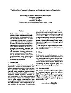
The first question to ask is how many local optima does the cost surface have using the standard features. A complex cost surface indicates that some gain may be had with non-linear features, but it also shows that special care should be taken during optimization. Non-convexity is revealed by sensitivity to initialization points. Thus, we decided to initialize from all vertices of the unit hypercube, and since we had 11 features, we ran 211 experiments. The histogram of BLEU scores on dev data after convergence is shown on Figure 1. We also plotted the histogram of an example dimension in Figure 2. The range of BLEU scores and lambdas is reasonably narrow. Even though λ seems to be bimodal, we see
that this does not seriously affect the BLEU score. This is not definitive evidence but we provisionally pretend that the cost surface is almost convex for practical purposes.
600
1 400 0.5 200 value
number of trained models
800
bins and re-trained. On Figure 3, we show that relaxing the monotonicity constraint leads to rough values for λ. Surprisingly, the BLEU score and objective on the training set only increases marginally. Starting from λ = 0, we obtained nearly exactly the same training objective value. By varying the number of bins (20-50), we observed similar behavior as well.
0 24.8 24.9
0 −0.5
25
25.1 25.2 25.3 25.4 BLEU score
Figure 1: Histogram of BLEU scores after training from 211 initializations.
−1 −1.5
original weights trained weights 0
10
20
30
40
50
bin id
Figure 3: Values before and after training bin features. Monotonicity constraint has been relaxed. BLEU score is virtually unchanged.
number of trained models
700 600 500 400 300 200 100 0
−60
−40
−20 λ value
0
Figure 2: Histogram of one λ parameter after training from 211 initializations. 4.3.2
Bin Features
A log-linear model can be converted into a bin feature model nearly exactly by setting λ values in such a way that scores will be equal. Equivalent weights (marked as ‘original’ in Figure 3) have the shape of an error function (erf): this is because the input feature is a cummulative random variable, which quickly converges to a Gaussian (by the central limit theorem). After training the λ weights for the log-linear model, weights may be converted into
4.3.3 GMM Features Experiments were carried out with GMM features. The summary is shown on Table 1. The baseline was the log-linear model trained with the baseline features. The baseline features are included in all systems. We trained GMM models using the iterative mixture splitting interleaved with EM reestimation, split up to 1024 and 16384 Gaussians, which we call GMM-ML-1k and GMM-ML-16k respectively. We also used the “perceptron” selection features on the training set to bootstrap quickly to 300k Gaussians (GMM-PCP-300k), and ran the same algorithm on the development set (GMMPCP-2k). Therefore, GMM-PCP-300k had 300k features, and was trained on 175k sentences (each with about 700 hypotheses). For all experiments but “unreg” (unregularized), we chose a prior Gaussian prior with variance empirically by looking at the development set. For all but GMM-PCP-300k, regularization did not seem to have a noticeably positive effect on development BLEU scores. All systems were seeded with the baseline log-linear model, and
all additional weights set to zero, and then trained with about 50 iterations, but convergence in BLEU score, empirical reward, and development BLEU score occurred after about 30 iterations. In that setting, we found that regularized empirical Bayes reward, BLEU score on training data, and BLEU score on development and evaluation to be well correlated. Cursory experiments revealed that using multiple initializations did not significantly alter the final BLEU score. System Oracle Baseline GMM-ML-1k GMM-ML-16k GMM-PCP-2k GMM-PCP-300k-unreg GMM-PCP-300k
Train 14.10 10.95 10.95 11.09 10.95 13.00 12.11
Dev N/A 35.15 35.15 35.25 35.15 N/A 35.74
Eval N/A 25.95 25.95 25.89 25.95 N/A 26.42
Table 1: BLEU scores for GMM features vs the linear baseline, using different selection methods and number of kernels. Perceptron kernels based on the training set improved the baseline by 0.5 BLEU points. We measured significance with the Wilcoxon signed rank test, by batching 10 sentences at a time to produce an observation. The difference was found to be significant at a 0.9-confidence level. The improvement may be limited due to local optima or the fact that original feature are well-suited for log-linear models.
5 Conclusion In this paper, we have introduced a non-parametric feature expansion, which guarantees invariance to the specific embodiment of the original features. Feature generation models, including feature expansion, may be trained using maximum regularized empirical Bayes reward. This may be used as an end-to-end framework to train all parameters of the machine translation system. Experimentally, we found that Gaussian mixture model (GMM) features yielded a 0.5 BLEU improvement. Although this is an encouraging result, further study is required on hyper-parameter re-estimation, presence of local optima, use of complex original
features to test the effectiveness of the parameterization invariance, and evaluation on a more competitive baseline.
References K. Papineni, S. Roukos, T. Ward, W.-J. Zhu. 2002. BLEU: a method for automatic evaluation of machine translation. ACL’02. A. Berger, S. Della Pietra, and V. Della Pietra. 1996. A Maximum Entropy Approach to Natural Language Processing. Computational Linguistics, vol 22:1, pp. 39–71. S. Chen and R. Rosenfeld. 2000. A survey of smoothing techniques for ME models. IEEE Trans. on Speech and Audio Processing, vol 8:2, pp. 37–50. R. O. Duda and P. E. Hart. 1973. Pattern Classification and Scene Analysis. Wiley & Sons, 1973. H. J. Kushner and G. G. Yin. 1997. Stochastic Approximation Algorithms and Applications. Springer-Verlag, 1997. National Institute of Standards and Technology. 2006. The 2006 Machine Translation Evaluation Plan. J. Nocedal and S. J. Wright. 1999. Numerical Optimization. Springer-Verlag, 1999. F. J. Och. 2003. Minimum Error Rate Training in Statistical Machine Translation. ACL’03. F. J. Och, D. Gildea, S. Khudanpur, A. Sarkar, K. Yamada, A. Fraser, S. Kumar, L. Shen, D. Smith, K. Eng, V. Jain, Z. Jin, and D. Radev. 2004. A Smorgasbord of Features for Statistical Machine Translation. HLT/NAACL’04. F. J. Och and H. Ney. 2002. Discriminative Training and Maximum Entropy Models for Statistical Machine Translation. ACL’02. D. Povey, B. Kingsbury, L. Mangu, G. Saon, H. Soltau and G. Zweig. 2004. fMPE: Discriminatively trained features for speech recognition. RT’04 Meeting. C. Quirk, A. Menezes and C. Cherry. 2005. Dependency Tree Translation: Syntactically Informed Phrasal SMT. ACL’05. L. R. Rabiner and B.-H. Huang. 1993. Fundamentals of Speech Recognition. Prentice Hall. M. Riedmiller and H. Braun. 1992. RPROP: A Fast Adaptive Learning Algorithm. Proc. of ISCIS VII. D. A. Smith and J. Eisner. 2006. Minimum-Risk Annealing for Training Log-Linear Models. ACLCOLING’06.