Tracking Down the Origins of Ambiguity in Context-Free Grammars H.J.S. Basten Centrum Wiskunde & Informatica P.O. Box 94079 NL-1090 GB Amsterdam, The Netherlands
Abstract. Context-free grammars are widely used but still hindered by ambiguity. This stresses the need for detailed detection methods that point out the sources of ambiguity in a grammar. In this paper we show how the approximative Noncanonical Unambiguity Test by Schmitz can be extended to conservatively identify production rules that do not contribute to the ambiguity of a grammar. We prove the correctness of our approach and consider its practical applicability.
1
Introduction
Context-free grammars (CFGs) are widely used in various fields, like for instance programming language development, natural language processing, or bioinformatics. They are suitable for the definition of a wide range of languages, but their possible ambiguity can hinder their use. Designed ambiguities are not uncommon, but accidentally introduced ambiguities are unwanted. Ambiguities are very hard to detect by hand, so automated ambiguity checkers are welcome tools. Despite the fact the CFG ambiguity problem is undecidable in general [5,7,6], various detection schemes exist. They can roughly be divided into two categories: exhaustive methods and approximative ones. Methods in the first category exhaustively search the usually infinite set of derivations of a grammar, while the latter ones apply approximation to limit their search space. This enables them to always terminate, but at the expense of potentially incorrect reports. Exhaustive methods do produce precise reports, but only if they find ambiguity before they are halted, because they obviously cannot be run forever. Because of the undecidability it is impossible to always terminate with a correct and detailed report. The challenge is to develop a method that gives the most precise answer in the time available. In this paper we propose to combine exhaustive and approximative methods as a step towards this goal. We show how to extend the Regular Unambiguity Test and Noncanonical Unambiguity Test [11] to improve the precision of their approximation and that of their ambiguity reports. The extension enables the detection of production rules that do not contribute to the ambiguity of a grammar. These are already helpful reports for the grammar developer, but can also be used to narrow the search space of other detection methods. In an earlier study [3] we witnessed significant reductions in the run-time of exhaustive methods due to our grammar filtering. A. Cavalcanti et al. (Eds.): ICTAC 2010, LNCS 6255, pp. 76–90, 2010. c Springer-Verlag Berlin Heidelberg 2010 �
Tracking Down the Origins of Ambiguity in Context-Free Grammars
1.1
77
Related Work
The original Noncanonical Unambiguity Test by Schmitz is an approximative test for the unambiguity of a grammar. The approximation it applies is always conservative, so it can only find a grammar to be unambiguous or potentially ambiguous. Its answers always concern the grammar as a whole, but the reports of a prototype implementation [12] by the author also contain clues about the production rules involved in the potential ambiguity. However, these are very abstract and hard to understand. The extensions that we present do result in precise reports, while remaining conservative. Another approximative ambiguity detection scheme is the “Ambiguity Checking with Language Approximation” framework [4] by Brabrand, Giegerich and Møller. The framework makes use of a characterization of ambiguity into horizontal and vertical ambiguity to test whether a certain production rule can derive ambiguous strings. The difference with our approach is that we test whether a production rule is vital for the existence of parse trees of ambiguous strings. 1.2
Overview
We start with background information about grammars and languages in Section 2. Then we repeat the definition of the Regular Unambiguity (RU) Test in Section 3. In Section 4 we explain how the RU Test can be extended to identify sets of parse trees of unambiguous strings. From these parse trees we can identify harmless production rules as explained in Section 5. Section 6 explains the Noncanonical Unambiguity (NU) Test, an improvement over the RU Test, and also shows how it improves the effect of our parse tree and production rule filtering. In Section 7 we describe how our approach can be used iteratively to increase its precision. Finally, Section 9 contains the conclusion. We prove our results in an accompanying technical report [2].
2
Preliminaries
This section gives a quick overview of the theory of grammars and languages, and introduces the notational convention used throughout this document. For more background information we refer to [9,14]. 2.1
Context-Free Grammars
A context-free grammar G is a 4-tuple (N, T, P, S) consisting of: – – – –
N , a finite set of nonterminals, T , a finite set of terminals (the alphabet), P , a finite subset of N × (N ∪ T )∗ , called the production rules, S, the start symbol, an element from N .
We use V to denote the set N ∪ T , and V � for V ∪ {ε}. The following characters are used to represent different symbols and strings: a, b, c, . . . represent terminals,
78
H.J.S. Basten
A, B, C, . . . represent nonterminals, X, Y , Z represent either nonterminals or terminals, α, β, γ, . . . represent strings in V ∗ , u, v, w, . . . represent strings in T ∗ , ε represents the empty string. A production (A, α) in P is written as A → α. We use the function pid : P → N to relate each production to a unique identifier. An item [10] indicates a position in the right hand side of a production using a dot. Items are written like A → α• β. The relation =⇒ denotes direct derivation, or derivation in one step. Given the string αBγ and a production rule B → β, we can write αBγ =⇒ αβγ (read αBγ directly derives αβγ). The symbol =⇒∗ means “derives in zero or more steps”. A sequence of derivation steps is simply called a derivation. Strings in V ∗ are called sentential forms. We call the set of sentential forms that can be derived from S of a grammar G, the sentential language of G, denoted S(G). A sentential form in T ∗ is called a sentence. The set of all sentences that can be derived from S of a grammar G is called the language of G, denoted L(G). We assume every nonterminal A is reachable from S, that is ∃αAβ ∈ S(G). We also assume every nonterminal is productive, meaning ∃u : A =⇒∗ u. The parse tree of a sentential form α describes how α is derived from S, but disregards the order of the derivation steps. To represent parse trees we use bracketed strings (See Section 2.3). A grammar G is ambiguous iff there is at least one string in L(G) for which multiple parse trees exist. 2.2
Bracketed Grammars
From a grammar G = (N, T, P, S) a bracketed grammar Gb can be constructed, by adding unique terminals to the beginning and end of every production rule [8]. The bracketed grammar Gb is defined as the 4-tuple (N, Tb , Pb , S), where: – – – –
Tb = T ∪ T� ∪ T� , T� = { �i | ∃p ∈ P : i = pid(p)}, T� = { �i | ∃p ∈ P : i = pid(p)}, Pb = {A → �i α�i | A → α ∈ P, i = pid(A → α)}.
Vb is defined as Tb ∪ N , and Vb� as Vb ∪ {ε}. We use ab , bb , . . . and Xb , Yb , Zb to represent symbols in respectively Tb and Vb . Similarly, ub , vb , . . . and αb , βb , . . . represent strings in respectively Tb∗ and Vb∗ , The relation =⇒b denotes direct derivation using productions in Pb . The homomorphism h from Vb∗ to V ∗ maps each string in S(Gb ) to S(G). It is defined by h(�i ) = ε, h(�i ) = ε, and h(X) = X. 2.3
Parse Trees
L(Gb ) describes exactly all parse trees of all strings in L(G). S(Gb ) describes exactly all parse trees of all strings in S(G). We divide it into two disjoint sets: Definition 1. The set of parse trees of ambiguous strings of G is P a (G) = {αb | αb ∈ S(Gb ), ∃βb ∈ S(Gb ) : αb = βb , h(αb ) = h(βb )}. The set of parse trees of unambiguous strings of G is P u (G) = S(Gb ) \ P a (G).
Tracking Down the Origins of Ambiguity in Context-Free Grammars
79
Example 1. Below is an example grammar (1) together with its bracketed version (2). The string aaa has two parse trees, �1 �2 �2 �3 a�3 �3 a�3 �2 �3 a�3 �2 �1 and �1 �2 �3 a�3 �2 �3 a�3 �3 a�3 �2 �2 �1 , and is therefore ambiguous. 1 : S → A, 2 : A → AA, 3:A→a 1 : S → �1 A�1 , 2 : A → �2 AA�2 , 3 : A → �3 a�3
(1) (2)
We call the set of the smallest possible ambiguous sentential forms of G the ambiguous core of G. These are the ambiguous sentential forms that cannot be derived from other sentential forms that are already ambiguous. Their parse trees are the smallest indicators of the ambiguities in G. Definition 2. The set of parse trees of the ambiguous core of a grammar G is C a (G) = {αb | αb ∈ P a (G), ¬∃βb ∈ P a (G) : βb =⇒b αb } From C a (G) we can obtain P a (G) by adding all sentential forms reachable with =⇒b . And since C a (G) ⊆ P a (G) we get the following Lemma: Lemma 1. A grammar G is ambiguous iff C a (G) is non-empty. Similar to P u (G), we define the complement of C a (G) as C u (G) = S(Gb )\C a (G), for which holds that P u (G) ⊆ C u (G). Example 2. The two parse trees �1 �2 �2 AA�2 A�2 �1 and �1 �2 A�2 AA�2 �2 �1 , of the ambiguous sentential form AAA, are in the ambiguous core of Grammar (1). 2.4
Positions
A position in a sentential form is an element in Vb∗ × Vb∗ . The position (αb , βb ) is written as αb • βb . pos(Gb ) is the set of all positions in strings of S(Gb ), defined as {αb • βb | αb βb ∈ S(Gb )}. Every position in pos(Gb ) is a position in a parse tree, and corresponds to an item of G. The item of a position can be identified by the closest enclosing �i and �i pair around the dot, considering balancing. For positions with the dot at the beginning or the end we introduce two special items • S and S • . We use the function item to map a position to its item. It is defined by item(γb • δb ) = A → α� • β � iff γb • δb = ηb �i αb • βb �i θb , A → �i α� β � �i ∈ Pb , α� =⇒∗b αb and β � =⇒∗b βb , item(• αb ) = • S, and item(αb • ) = S • . Another function items returns the set of items used at all positions in a parse tree. It is defined as items(αb ) = {A → α• β | ∃γb • δb : γb δb = αb , A → α• β = item(γb • δb )}. Example 3. The following shows the parse tree representations of the positions �1 �2 • �3 a�3 �3 a�3 �2 �1 and �1 �2 �3 a�3 • �3 a�3 �2 �1 . We see that the first position is at item A → • AA and the second is at A → A• A.
•
S
S
A
A
A
A
A
a
a
a
•
A a
80
H.J.S. Basten
The function proditems maps a production rule to the set of all its items. It is defined as proditems(A → α) = {A → β • γ | βγ = α}. If a production rule is used to construct a parse tree, then all its items occur at one or more positions in the tree. Lemma 2. ∀αb �i βb �i γb ∈ S(Gb ) : ∃A → δ ∈ P : pid(A → δ) = i, proditems(A → δ) ⊆ items(αb �i βb �i γb ). 2.5
Automata
An automaton A is a 5-tuple (Q, Σ, R, Qs , Qf ) where Q is the set of states, Σ is the input alphabet, R in Q × Σ × Q is the set of rules or transitions, Qs ⊆ Q is the set of start states, and Qf ⊆ Q is the set of final states. A a transition (q0 , a, q1 ) is written as q0 −→ q1 . The language of an automaton is the set of strings read on all paths from a start state to an end state. Formally, α L(A) = {α | ∃qs ∈ Qs , qf ∈ Qf : qs −→∗ qf }.
3
Regular Unambiguity Test
This section introduces the Regular Unambiguity (RU) Test [11] by Schmitz. The RU Test is an approximative test for the existence of two parse trees for the same string, allowing only false positives. 3.1
Position Automaton
The basis of the Regular Unambiguity Test is a position automaton, which describes all strings in S(Gb ). The states of this automaton are the positions in pos(Gb ). The transitions are labeled with elements from Vb . Definition 3. The position automaton1 Γ (G) of a grammar G is the tuple (Q, Vb , R, Qs , Qf ), where – – – –
Q = pos(Gb ), Xb R = {αb • Xb βb −→ αb Xb • βb | αb Xb βb ∈ S(Gb )}, • Qs = { αb | αb ∈ S(Gb )}, Qf = {αb • | αb ∈ S(Gb )}.
There are three types of transitions: derives with labels in T� , reduces with labels in T� , and shifts of terminals and nonterminals in V . The symbols read on a path through Γ (G) describe a parse tree of G. Thus, L(Γ (G)) = S(Gb ). Γ (G) contains a unique subgraph for each string in S(Gb ). The string read by a subgraph can be identified by the positions on the nodes of the subgraph. Every position dictates the prefix read up until its node, and the postfix required to reach the end state of its subgraph. Therefore, every path that corresponds to a string in L(Γ (G)) must pass all positions of that string. 1
We modified the original definition of the position automaton to be able to explain our extensions more clearly. This does not essentially change the RU Test and NU Test however, since their only requirement on Γ (G) is that it defines S(Gb ).
Tracking Down the Origins of Ambiguity in Context-Free Grammars
81
Lemma 3. ∀αb , βb : αb • βb ∈ Q ⇔ αb βb ∈ L(Γ (G)). A grammar G is ambiguous iff two paths exist through Γ (G) that describe different parse trees in P a (G) — strings in S(Gb ) — of the same string in S(G). We call such two paths an ambiguous path pair. Example 4. The following shows the first part of the position automaton of the grammar from Example 1. It shows paths for parse trees S, �1 A�1 and �1 �3 a�3 �1 . •
•
•
�1 �3 a�3 �1
3.2
�1
�1 A�1
�1 • �3 a�3 �1
�1 �3
S
�1 • A�1 �1 �3 • a�3 �1
S A a
S• �1
�1 A • �1
�3
�1 �3 a • �3 �1
�1 A�1 • �1 �3 a�3 • �1
�1
�1 �3 a�3 �1 •
Approximated Position Automaton
If G has an infinite number of parse trees, the position automaton is also of infinite size. Checking it for ambiguous path pairs would take forever. Therefore the position automaton is approximated using equivalence relations on the positions. The approximated position automaton has equivalence classes of positions for its states. For every transition between two positions in the original automaton a new transition with the same label then exists between the equivalence classes that the positions are in. If an equivalence relation is used that yields a finite set of equivalence classes, the approximated automaton can be checked for ambiguous path pairs in finite time. Definition 4. Given an equivalence relation ≡ on positions, the approximated position automaton Γ≡ (G) of the automaton Γ (G) = (Q, Vb , R, Qs , Qf ), is the tuple (Q≡ , Vb� , R≡ , {qs }, {qf }) where – Q≡ = Q/≡ ∪ {qs , qf }, where Q/≡ is the set of non-empty equivalence classes over pos(Gb ) modulo ≡, defined as {[αb • βb ]≡ | αb • βb ∈ Q}, X
X
ε
ε
b b [q1 ]≡ | q0 −→ q1 ∈ R} ∪ {qs −→ [q]≡ | q ∈ Qs } ∪ {[q]≡ −→ – R≡ = {[q0 ]≡ −→ qf | q ∈ Qf }, – qs and qf are respectively the start and final state.
The paths through Γ≡ (G) describe an overapproximation of the set of parse trees of G, thus L(Γ (G)) ⊆ L(Γ≡ (G)). So if no ambiguous path pair exists in Γ≡ (G), grammar G is unambiguous. But if there is an ambiguous path pair, it is unknown if its paths describe real parse trees of G or approximated ones. In this case we say G is potentially ambiguous. The item0 Equivalence Relation. Checking for ambiguous paths in finite time also requires an equivalence relation with which Γ≡ (G) can be built in finite
82
qs
H.J.S. Basten
ε
•
S
S
S•
�1
ε
qf
�1 A
S → •A
�2 �2
A → • AA �3
S → A•
�2
�3
A �2
A → •a
A → A• A �3
�3 a
A �2
�2
A → AA• �3
�3
A → a•
Fig. 1. The item0 position automaton of the grammar of Example 1
time. A relation like that should enable the construction of the equivalence classes without enumerating all positions in pos(Gb ). A simple but useful equivalence relation with this property is the item0 relation [11]. Two positions are equal modulo item0 if they are both at the same item. Definition 5. αb • βb item0 γb • δb iff item(αb • βb ) = item(γb • δb ). Intuitively the item0 position automaton Γitem0 (G) of a grammar resembles that grammar’s LR(0) parse automaton [10]. The nodes are the LR(0) items of the grammar and the X and � edges correspond to the shift and reduce actions in the LR(0) automaton. The � edges do not have LR(0) counterparts. Every item with the dot at the beginning of a production of S is a start node, and every item with the dot at the end of a production of S is an end node. The difference between an LR(0) automaton and an item0 position automaton is in the reductions. Γitem0 (G) has reduction edges to every item that has the dot after the reduced nonterminal, while an LR(0) automaton jumps to a different state depending on the symbol that is at the top of the parse stack. As a result, a certain path through Γitem0 (G) with a �i transition from A → α• Bγ does not necessarily need to have a matching �i transition to A → αB • γ. Example 5. Figure 1 shows the item0 position automaton of the grammar of Example 1. Strings �1 �2 �3 a�3 �1 and �1 �3 a�3 �1 form an ambiguous path pair. The item0 relation can be combined with the lookk relation to get position automata that resemble LR(k) automata. This results in the itemk relation, which groups positions if they are equal modulo both item0 and lookk . Two positions are equal modulo lookk if their first k terminal symbols after the dot are identical. Definition 6. αb • βb lookk γb • δb iff (∃u, v, w : h(βb ) = uv, h(δb ) = uw, |u| = k) ∨ (h(βb ) = h(δb ) ∧ |h(βb )| < k).
Tracking Down the Origins of Ambiguity in Context-Free Grammars
83
The RU Test becomes more precise with increasing k values, because then Γitemk (G) better approximates S(G). 3.3
Position Pair Automaton
The existence of ambiguous path pairs in a position automaton can be checked with a position pair automaton, in which every state is a pair of states from the position automaton. Transitions between pairs are described using the mutual accessibility relation ma. R Definition 7. The regular position pair automaton Π≡ (G) of Γ≡ (G) is the 2 �2 2 2 2 �2 2 → , is the tuple (Q≡ , Vb , ma, qs , qf ), where ma over Q≡ × Vb × Q≡ , denoted by − → − union of the following subrelations: (�i ,ε)
�i
(X,X)
X
(�i ,ε)
�i
→ q2 }, maDl = {(q0 , q1 ) −−−→ (q2 , q1 ) | q0 − −−−→ �i (ε,�i ) → q3 }, maDr = {(q0 , q1 ) − −− −− −→ → (q0 , q3 ) | q1 −
X
maS = {(q0 , q1 ) − −− −− −− −→ → (q2 , q3 ) | q0 −→ q2 ∧ q1 −→ q3 , X ∈ V � },
maRl = {(q0 , q1 ) −−−→ (q2 , q1 ) | q0 − → q2 }, −−−→ �i (ε,�i ) → q3 }. maRr = {(q0 , q1 ) − −− −− −→ → (q0 , q3 ) | q1 −
Every path through this automaton from qs2 to qf2 describes two paths through R (G) is thus a set of pairs Γ≡ (G) that shift the same symbols. The language of Π≡ of strings. A path indicates an ambiguous path pair if its two bracketed strings are different, but equal under the homomorphism h. Because L(Γ≡ (G)) is an R over-approximation of S(Gb ), L(Π≡ (G)) contains at least all ambiguous path pairs through Γ (G). R (G)). Lemma 4. ∀αb , βb ∈ P a (G) : αb = βb ∧ h(αb ) = h(βb ) ⇒ (αb , βb ) ∈ L(Π≡
4
Finding Parse Trees of Unambiguous Strings
The Regular Unambiguity Test described in the previous section can conservatively detect the unambiguity of a given grammar. If it finds no ambiguity we are done, but if it finds potential ambiguity this report is not detailed enough to be useful. In this section we show how the RU Test can be extended to identify parse trees of unambiguous strings. These will form the basis of more detailed ambiguity reports, as we will see in Section 5. 4.1
Unused Positions
From the states of Γ≡ (G) that are not used on ambiguous path pairs, we can identify parse trees of unambiguous strings. For this we use the fact that every bracketed string that represents a parse tree of G must pass all its positions on its path through Γ (G) (Lemma 3). Therefore, all positions in states of Γ≡ (G) R that are not used by any ambiguous path pair through Π≡ (G) are positions in parse trees of unambiguous strings.
84
H.J.S. Basten
S(Gb ) L(Γ≡ (G))
P u (G) P a (G) u P≡ (G)
Fig. 2. Venn diagram showing the relationship between S(Gb ) and L(Γ≡ (G)). The vertical lines divide both sets in two: their parse trees of ambiguous strings (left) and parse trees of unambiguous strings (right).
Definition 8. The set of states of Γ≡ (G) that are used on ambiguous path pairs R through Π≡ (G) is Qa≡ = (αb ,α� )
(βb ,β � )
b ∗ {q0 , q1 | ∃αb , βb , α�b , βb� : αb βb = α�b βb� , qs2 −−−−− → (q0 , q1 ) −−−−b→∗ qf2 }. −−−−−→ −−−−→ The set of states not used on ambiguous path pairs is Qu≡ = Q≡ \ Qa≡ .
Definition 9. The set of parse trees of unambiguous strings of G that are idenu tifiable with ≡, is P≡ (G) = {αb βb | ∃q ∈ Qu≡ : αb • βb ∈ q}. This set is always a subset of P u (G), as illustrated by Fig. 2. u (G) ⊆ P u (G). Theorem 1. For all equivalence relations ≡, P≡
The positions in the states in Qa≡ and Qu≡ thus identify parse trees of respectively potentially ambiguous strings and certainly unambiguous strings. However, iterating over all positions in pos(G) is infeasible if this set is infinite. The used equivalence relation should therefore allow the direct identification of parse trees from the states of Γ≡ (G). For instance, a state in Γitem0 (G) represents all parse trees in which a particular item appears. With this information we can identify production rules that only u (G), as we will show in the next section. appear in parse trees in P≡ 4.2
Join Points
Gathering Qa≡ is also impossible in practice because it requires the inspection of all paths through Γ≡ (G), of which there can be infinitely many. We therefore need a definition that can be calculated in finite time. For this we use the notion R of join points. These are the points in Π≡ (G) where we see that two different paths through Γ≡ (G) potentially come together in the same state. R Definition 10. The set of join points J in Π≡ (G), over Q2≡ × Q2≡ , is defined (Xb ,X � )
as J = {((q0 , q1 ), (q2 , q2 )) | (q0 , q1 ) −−−−−b→ (q2 , q2 ), q0 = q1 , Xb ∈ T� ∨ Xb� ∈ T� }. −−−−−→ With J we then define the following alternative to Qa≡ :
Tracking Down the Origins of Ambiguity in Context-Free Grammars
85
R Definition 11. The set of states in Γ≡ (G) that are used in pairs of Π≡ (G) that a� can reach, or can be reached by, a join point, is Q≡ = ∗ ∗ ∗ ∗ 2 {q0 , q1 | ∃(p0 , p1 ) ∈ J : qs2 − → → → → → (q0 , q1 ) − − → p0 ∨ p1 − − → (q0 , q1 ) − − → qf }. −
This is a safe over-approximation of Qa≡ , because all ambiguous path pairs through Γ≡ (G) will eventually join in a certain state. It can be calculated by R iterating over the edges of Π≡ (G) to collect J, and then computing the images ∗ of the join points through ma and (ma−1 )∗ . Both steps are linear in the number R (G) (see [14] Chapter 2), which is worst case O(|Q≡ |4 ). of edges in Π≡
5
Harmless Production Rules
In this section we show how we can use Qa≡ to identify production rules that do not contribute to the ambiguity of G. These are the production rules that can never occur in parse trees of ambiguous strings. We call them harmless production rules. 5.1
Finding Harmless Production Rules
u (G). A production rule is certainly harmless if it is only used in parse trees in P≡ We should therefore search for productions that are never used on ambiguous R path pairs of Π≡ (G) that describe valid parse trees in G. We can find them by looking at the items of the positions in the states of Qa≡ . If not all items of a production rule are used then the rule cannot be used in a valid string in P a (G) (Lemma 2), and we know it is harmless.
Definition 12. The set of items used on the ambiguous path pairs through R a Π≡ (G) is I≡ = {A → α• β | ∃q ∈ Qa≡ : ∃γb • δb ∈ q : A → α• β = item(γb • δb )}. With it we can identify production rules of which all items are used: Definition 13. The set of potentially harmful production rules of G, identifiable R a (G), is Phf = {A → α | proditems(A → α) ⊆ I≡ }. from Π≡ Because of the approximation it is uncertain whether or not they can really be used to form valid parse trees of ambiguous strings. Nevertheless, all the other productions in P will certainly not appear in parse trees of ambiguous strings. Definition 14. The set of harmless production rules of G, identifiable from R (G), is Phl = P \ Phf . Π≡ Theorem 2. ∀p ∈ Phl : ¬∃αb �i βb �i γb ∈ P a (G) : i = pid(p). Example 6 in Section 7 shows finding Phl for a small grammar.
86
5.2
H.J.S. Basten
Complexity
R Finding Phf comes down to building Π≡ (G), finding Qa� ≡ , and enumerating all a� a positions in all classes in Q≡ to find I≡ . The number of these classes is finite, but the number of positions might not be. It would therefore be convenient if the a definition of the chosen equivalence relation could be used to collect I≡ in finitely many steps. With the item0 relation this is possible, because all the positions in a class are all in the same item. R (G) can be done in O(|G|2 ) (see [11]), where |G| is the Constructing Πitem 0 � number of items of G. After that, Qaitem0 can be gathered in O(|G|4 ), because |Qitem0 | is linear with |G|. Since this is the most expensive step, the worst case complexity of finding Phf with item0 is therefore also O(|G|4 ).
5.3
Grammar Reconstruction
Finding Phl can be very helpful information for the grammar developer. Also, Phf represents a smaller grammar that can be checked again more easily to find the true origins of ambiguity. However, the reachability and productivity properties of this smaller grammar might be violated because of the removed productions in Phl . To restore these properties we have to introduce new terminals and productions, and a new start symbol. We must prevent introducing new ambiguities in this process. From Phf we can create a new grammar G� by constructing: 1. The set of defined nonterminals of Phf : Ndef = {A | A → α ∈ Phf }. 2. The used but undefined nonterminals of Phf : Nundef = {B | A → αBβ ∈ Phf }\Ndef . 3. The unproductive nonterminals: Nunpr = {A | A ∈ Ndef , ¬∃u : A =⇒∗ u using only productions in Phf }. 4. The start symbols of Phf : Shf = {A | A ∈ Ndef , ¬∃B → βAγ ∈ Phf }. 5. New terminal symbols tA , bA , eA for each nonterminal A. 6. New productions to define a new start-symbol S � : PS � = {S � → bA AeA | A ∈ Shf }. 7. Productions to complete the unproductive and undefined nonterminals: P � = Phf ∪ PS � ∪ {A → tA | A ∈ Nundef ∪ Nunpr}. 8. The new set of terminal symbols: T � = {a | A → βaγ ∈ P � }. 9. Finally, the new grammar: G� = (Ndef ∪ Nundef ∪ {S � }, T � , P � , S � ). Surrounding the nonterminals in Shf with unique terminals at step 6 prevents the new rules of S � from being ambiguous with each other. The unique terminals at step 7 make sure we do not create new parse trees for existing strings in L(G).
6
Noncanonical Unambiguity Test
In this section we explain the Noncanonical Unambiguity (NU) Test [11], which is more precise than the Regular Unambiguity Test. It enables the identification of a larger set of irrelevant parse trees, namely the ones in C u (G). From these we can also identify a larger set of harmless production rules and tree patterns.
Tracking Down the Origins of Ambiguity in Context-Free Grammars
6.1
87
Improving the Regular Unambiguity Test
The regular position pair automaton described in Section 3 checks all pairs of paths through a position automaton for ambiguity. However, it also checks some spurious paths that are unnecessary for identifying the ambiguity of a grammar. These are the path pairs that derive the same unambiguous substring for a certain nonterminal. We can ignore these paths because in this situation there are also two paths in which the nonterminal was shifted instead of derived. For instance, consider paths �1 �2 �3 a�3 αb �2 �1 and �1 �2 �3 a�3 βb �2 �1 . If they form R a pair in L(Π≡ (G)) then the shorter paths �1 �2 Aαb �2 �1 and �1 �2 Aβb �2 �1 will too (considering A → �3 a�3 ∈ Pb ). In addition, if the first two paths form an ambiguous path pair, then these latter two will also, because �3 a�3 does not contribute to the ambiguity. In this case we prefer the latter paths because they describe smaller parse trees than the first paths. 6.2
Noncanonical Position Pair Automaton
To avoid common unambiguous substrings we should only allow path pairs to take identical reduce transitions if they do not share the same substring since their last derives. To keep track of this property we add two extra boolean flags c0 and c1 to the position pairs. These flags tell for each position in a pair whether or not its path has been in conflict with the other, meaning it has taken different reduce steps as the other path since its last derive. A value of 0 means this has not occurred yet, and we are thus allowed to ignore an identical reduce transition. All start pairs have both flags set to 0, and every derive step resets the flag of a path to 0. The flag is set to 1 if a path takes a conflicting reduce step, which occurs if the other path does not follow this reduce at the same time (for instance �2 in the parse trees �1 �2 �3 a�3 �2 �1 and �1 �2 �3 a�3 �1 ). We use the predicate confl (called eff by Schmitz) to identify a situation like that. u
uX
confl(q, i) = ∃u ∈ T�∗ : q −→∗ qf ∨ (∃q � ∈ Q≡ , X ∈ V ∪ T� : X =�i , q −→+ q � ) (3) It tells whether there is another shift or reduce transition other than �i possible from q, ignoring � steps, or if q is at the end of the automaton. N (G) of Γ≡ (G) is Definition 15. The noncanonical position pair automaton Π≡ p �2 2 2 p the tuple (Q , Vb , nma, (qs , 0) , (qf , 1) ), where Q = (Q≡ × B)2 , and nma over Qp × Vb�2 × Qp is the noncanonical mutual accessibility relation, defined as the union of the following subrelations: (�i ,ε)
�i
(�i ,ε)
�i
→ q2 }, nmaDl = {(q0 , q1 )c0 , c1 − −− −− −→ → (q2 , q1 )0, c1 | q0 − (ε,�i ) �i nmaDr = {(q0 , q1 )c0 , c1 −−−→ (q0 , q3 )c0 , 0 | q1 − → q3 }, −−−→ (X,X) X X → q2 , q1 −→ q3 , X ∈ V � }, nmaS = {(q0 , q1 )c0 , c1 − −− −− −− −→ → (q2 , q3 )c0 , c1 | q0 − nmaCl = {(q0 , q1 )c0 , c1 − −− −− −→ → (q2 , q1 )1, c1 | q0 −→ q2 , confl(q1 , i)}, (ε,�i ) �i nmaCr = {(q0 , q1 )c0 , c1 −−−→ (q0 , q3 )c0 , 1 | q1 −→ q3 , confl(q0 , i)}, −−−→ (�i ,�i ) �i �i → q2 , q1 −→ q3 , c0 ∨ c1 }. nmaR = {(q0 , q1 )c0 , c1 − −− −− −− −→ → (q2 , q3 )1, 1 | q0 −
88
H.J.S. Basten
R N As with Π≡ (G), the language of Π≡ (G) describes ambiguous path pairs N through Γ≡ (G). The difference is that L(Π≡ (G)) does not include path pairs N R without conflicting reductions. Therefore L(Π≡ (G)) ⊆ L(Π≡ (G)). Nevertheless, N a Π≡ (G) does at least describe all the core parse trees in C (G): N (G)). Theorem 3. ∀αb , βb ∈ C a (G) : αb = βb ∧ h(αb ) = h(βb ) ⇒ (αb , βb ) ∈ L(Π≡
The Theorem shows that if G is ambiguous — that is C a (G) is non-empty — N N L(Π≡ (G)) is also non-empty. This means that if L(Π≡ (G)) is empty, G is unambiguous. 6.3
Effects on Filtering Parse Trees and Production Rules
The new nma relation enables our parse tree identification algorithm of Section 4 to potentially identify a larger set of irrelevant parse trees, namely C u (G). These trees might be ambiguous, but this is not a problem because we are interested in finding the trees of the smallest possible sentential forms of G, namely the ones in C a (G). N (G), the set of parse trees not in the amDefinition 16. Given Qu≡ from Π≡ u biguous core of G, identifiable with ≡, is C≡ (G) = {αb βb | ∃q ∈ Qu≡ , αb • βb ∈ q}. u (G) ⊆ C u (G). Theorem 4. For all equivalence relations ≡, C≡ N (G) is also The set of harmless production rules that can be identified with Π≡ potentially larger. It might include rules that can be used in parse trees of ambiguous strings, but not in parse trees in C a (G). Therefore they are not vital for the ambiguity of G. a N from Π≡ (G), the set of harmless productions Definition 17. Given Qa≡ and I≡ N � a of G, identifiable from Π≡ (G), is Phl = P \ {A → α | proditems(A → α) ⊆ I≡ }. � : ¬∃αb �i βb �i γb ∈ C a (G) : i = pid(p). Theorem 5. ∀p ∈ Phl
7
Excluding Parse Trees Iteratively
Our approach for the identification of parse trees of unambiguous strings is most useful if applied in an iterative setting. By checking the remainder of the potentially ambiguous parse trees again, there is possibly less interference of the trees during approximation. This could result in less ambiguous path pairs in the position pair automaton. We could then exclude a larger set of parse trees and production rules. Example 6. The grammar below (4) is unambiguous but needs two iterations N (G) contains only the of the NU Test with item0 to detect this. At first, Πitem 0 ambiguous path pair �1 �4 c�4 �1 and �2 �5 �6 c�6 �3 �1 . The first path describes a valid parse tree, but the second does not. From B → • Cb it derives to C → • c, but
Tracking Down the Origins of Ambiguity in Context-Free Grammars
89
Table 1. Excerpt from Results of prototype implementation Grammar Harmless rules Time Amber Time CfgAnalyzer Name Rules LR(0) SLR(1) LR(1) Original Filtered Original Filtered SQL.1 79 65 65 65 28m26s 0.1s 17.6s 1.8s 21 30 144 31.8s 0.0s 9.6s 1.3s Pascal.3 176 41 44 44 4.5h1 4.12s1 3.0h 1.1h C.2 212 2 56 70 74 25.0h 22m52s2 48.9s 32.4s Java.1 349 1 for sentences of length 7 (first ambiguity at length 13) 2 for sentences of length 12 (first ambiguity at length 13)
from C → c• it reduces to A → aC • . Therefore productions 2, 5 and 3 are only used partially, and they are thus harmless. After removing them and checking the reconstructed grammar again there are no ambiguous path pairs anymore. 1 : S → A, 2 : S → B, 3 : A → aC, 4 : A → c, 5 : B → Cb, 6 : C → c
(4)
We can gain even higher precision by choosing a new equivalence relation with each iteration. If with each step Γ≡ (G) better approximates S(Gb ), we might end up with only the parse trees in P u (G). Unfortunately, the ambiguity problem is undecidable, and this process does not necessarily have to terminate. There might be an infinite number of equivalence relations that yield a finite number of equivalence classes. Or at some point we might need to resort to equivalence relations that do not yield a finite graph. Therefore, the iteration has to stop at a certain moment, and we can continue with an exhaustive search of the remaining parse trees. In the end this exhaustive searching is the most practical, because it can point out the exact parse trees of ambiguous strings. A drawback of this approach is its exponential complexity. Nevertheless, excluding sets of parse trees beforehand can reduce its search space significantly, as we see in the next section.
8
Prototype Results
In [3] we tested a prototype implementation of our approach on a collection of programming language grammars. From unambiguous grammars of SQL, Pascal, C and Java, we created 5 ambiguous versions for each language. For each grammar we tested the number of harmless production rules we could find with the NU Test, using different equivalence relations. Columns 3-5 of Table 1 show the results of these tests for a selection of 4 ambiguous grammars. Similar numbers of harmless rules could be found for the other grammars. Columns 7-9 show the effect that the removal of the harmless productions had on the run-time of the two exhaustive derivation generators Amber [13] and CfgAnalyzer [1]. They mention the time needed to find the first ambiguous derivation of a grammar before and after filtering with LR(1). We see significant reductions in run-time, sometimes orders of magnitude. For the other grammars we witnessed similar effects.
90
H.J.S. Basten
9
Conclusions
We showed how the Regular Unambiguity Test and Noncanonical Unambiguity Test can be extended to conservatively identify parse trees of unambiguous strings. From these trees we can identify production rules that do not contribute to the ambiguity of the grammar. This information is already very useful for a grammar developer, but it can also be used to significantly reduce the search space of other ambiguity detection methods.
References 1. Axelsson, R., Heljanko, K., Lange, M.: Analyzing context-free grammars using an incremental SAT solver. In: Aceto, L., Damg˚ ard, I., Goldberg, L.A., Halld´ orsson, M.M., Ing´ olfsd´ ottir, A., Walukiewicz, I. (eds.) ICALP 2008, Part II. LNCS, vol. 5126, pp. 410–422. Springer, Heidelberg (2008) 2. Basten, H.J.S.: Tracking down the origins of ambiguity in context-free grammars. Tech. Rep. SEN-1005, CWI, Amsterdam, The Netherlands (2010) 3. Basten, H.J.S., Vinju, J.J.: Faster ambiguity detection by grammar filtering. In: Proceedings of the Tenth Workshop on Language Descriptions, Tools and Applications (LDTA 2010). ACM, New York (2010) 4. Brabrand, C., Giegerich, R., Møller, A.: Analyzing ambiguity of context-free grammars. Science of Computer Programming 75(3), 176–191 (2010) 5. Cantor, D.G.: On the ambiguity problem of Backus systems. Journal of the ACM 9(4), 477–479 (1962) 6. Chomsky, N., Sch¨ utzenberger, M.: The algebraic theory of context-free languages. In: Braffort, P. (ed.) Computer Programming and Formal Systems, pp. 118–161. North-Holland, Amsterdam (1963) 7. Floyd, R.W.: On ambiguity in phrase structure languages. Communications of the ACM 5(10), 526–534 (1962) 8. Ginsburg, S., Harrison, M.A.: Bracketed context-free languages. Journal of Computer and System Sciences 1(1), 1–23 (1967) 9. Hopcroft, J.E., Ullman, J.D.: Introduction to Automata Theory, Languages and Computation. Addison-Wesley, Reading (1979) 10. Knuth, D.E.: On the translation of languages from left to right. Information and Control 8(6), 607–639 (1965) 11. Schmitz, S.: Conservative ambiguity detection in context-free grammars. In: Arge, L., Cachin, C., Jurdzi´ nski, T., Tarlecki, A. (eds.) ICALP 2007. LNCS, vol. 4596, pp. 692–703. Springer, Heidelberg (2007) 12. Schmitz, S.: An experimental ambiguity detection tool. Science of Computer Programming 75(1-2), 71–84 (2010) 13. Schr¨ oer, F.W.: AMBER, an ambiguity checker for context-free grammars. Tech. rep., compilertools.net (2001), http://accent.compilertools.net/Amber.html 14. Sippu, S., Soisalon-Soininen, E.: Parsing theory. Languages and parsing, vol. 1. Springer, New York (1988)