Tilted Nonparametric Estimation of Volatility Functions with Empirical Applications∗ Ke-Li Xu† and Peter C. B. Phillips‡ January 15, 2009

Abstract This paper proposes a novel positive nonparametric estimator of the conditional variance function without reliance on logarithmic or other transformations. The estimator is based on an empirical likelihood modification of conventional local level nonparametric regression applied to squared mean regression residuals. The estimator is shown to be asymptotically equivalent to the local linear estimator but is restricted to be non-negative in finite samples. It is fully adaptive to the unknown conditional mean function. Simulations are conducted to evaluate finite sample performance of the estimator. Two empirical applications are reported. One uses cross section data and studies the relationship between occupational prestige and income. The other uses time series data on Treasury bill rates to fit the total volatility function in a continuous time jump diffusion model. ∗

The authors thank Taisuke Otsu for helpful comments. Xu acknowledges partial research support from University of Alberta School of Business under the H. E. Pearson fellowship and the J. D. Muir grant. Phillips acknowledges partial research support from a Kelly Fellowship and the NSF under Grant Nos. SES 04-142254 and 06-47086. † Department of Finance and Management Science, University of Alberta School of Business. Address: Business Building 3-40N, University of Alberta School of Business, Edmonton, Alberta, Canada, T6G 2R6. E-mail address: [email protected]. ‡ Yale University, University of Auckland, University of York and Singapore Management University. Address: Department of Economics, Cowles Foundation for Research in Economics, Yale University, P. O. Box 208281, New Haven, CT 06520, USA. E-mail address: [email protected].

1

JEL Classification: C13; C14; C22.

Keywords: Conditional variance function; Empirical likelihood; Conditional heteroskedasticity; Jump diffusions; Local linear estimator; Heteroskedastic nonparametric regression; Volatility.

1

Introduction

Conditional variance estimation is important in many applications. It is crucial in inference for the parameters in the conditional mean function. For example, to test for the causal treatment effect in a regression discontinuity design (Porter, 2003, Imbens and Lemieux, 2008), the conditional variances of the outcome variable on the running variable at the threshold have to be estimated. Hansen (1995) obtained GLS-type efficient estimators of parameters in the mean function by incorporating nonparametric conditional variance estimates; see also Xu and Phillips (2008). Conditional variance estimation is also a key intermediate step in estimating some economic or financial quantities of practical importance. In a recent study, Martins-Filho and Yao (2007) proposed a nonparametric method to estimate production frontier function starting from estimation of the conditional variance of the output given the input. Shang (2008) provided a two-stage value-at-risk forecasting procedure in a nonparametric ARCH framework based on first estimation the volatility function (viz. conditional standard deviation) and then quantile estimation using the devolatized residuals. When the conditional variance is modeled nonparametrically, as in the applications mentioned above, the estimating methods usually recommended are based on local polynomial estimation, among which local linear estimation is especially popular due to its many nice properties. The theoretical foundation to justify this has been built up by Ruppert et al. (1997) and Fan and Yao (1998), inter alia. However, one drawback of the local linear

2

variance estimator, which doesn’t exist in the local linear mean function estimator, is that it may give negative values in finite samples which makes volatility estimation impossible. Negative variance estimates may happen for large or small smoothing bandwidths and are frequently observed at design points around which observations are relatively sparse. In consequence, it is commonly recommended in applications to use the theoretically less satisfactory local constant estimator (also known as Nadaraya-Watson estimator) when fitting the variance function (Chen and Qin, 2002, Porter, 2003). This paper proposes a new volatility function estimator that is almost asymptotically equivalent to the local linear estimator but is guaranteed to be non-negative. It has the same asymptotic bias and variance as those of the local linear estimator when the explanatory variable has unbounded support. Such equivalence is important since it renders efficiency arguments along the lines of of Fan (1992) for the local linear estimator extendable to this analog. It is also convenient in that the mean square errors (MSE) or integrated MSE based selection criteria of a global or local variable bandwidth are also usable. The new volatility function estimator is based on the idea of adjusting the conventional local constant estimator by minimally tilting the empirical distribution subject to a discrete bias-reducing moment condition satisfied by the local linear estimator (Hall and Presnell, 1999). The resultant re-weighted local constant, or tilted estimator, inherits the non-negativity restriction of the variance function from the usual local constant estimator, while preserving the superior properties of bias, boundary correction and minimax efficiency of the local linear estimator. We also show adaptiveness of this procedure to the unknown mean function, i.e. it estimates the volatility function as efficiently as if the true mean function is known. Ziegelmann (2002) recently obtained a non-negative nonparametric volatility estimator by fitting an exponential function locally (rather than a linear function as in the local linear estimator) within the general locally parametric nonparametric framework of Hjort and Jones (1996); see also Yu and Jones (2004) in a Gaussian iid setting. This estimator is not equivalent to the local linear estimator and it essentially estimates the logarithm of 3

the variance rather than the variance itself, thus leading to an additional bias term. The remainder of the paper is organized as follows. Section 2.1 describes the nonparametric heteroskedastic regression model, the framework within which the re-weighted local constant is introduced in Section 2.2. The asymptotic distributional theory is developed for stationary and mixing time series in Section 2.3 for both interior and boundary points, and a consistent estimator of the asymptotic variance is suggested. In Section 3 the finite sample performance of the proposed estimator is evaluated via simulations. Section 4 reports two empirical applications. One studies the volatility of the relationship between income and occupational prestige in Canada using cross section data. The other estimates the total volatility of 90 day Treasury bill yields in the context of a continuous time jump diffusion model. Section 5 concludes and discusses some extensions. Proofs are collected in the appendix.

2 2.1

Main Results The heteroskedastic regression model

We focus on the following nonparametric heteroskedastic regression model

Yt = m(Xt ) + σ(Xt )εt ,

(1)

where {Xt , Yt , t = 1, · · · , T } are two stationary random processes, and {εt } are innovations satisfying E(εt |Xt ) = 0, V ar(εt |Xt ) = 1. The conditional mean function m(x) = E(Yt |Xt = x) and the conditional variance function σ 2 (x) = V ar(Yt |Xt = x) > 0 are left unspecified and are the focus of statistical investigation. The reader should keep in mind that the volatility estimator proposed below applies straightforwardly to the zero mean case, e.g. the nonparametric ARCH (1) model when Xt = Yt−1 (Pagan and Schwert, 1990, Pagan and Hong, 1991). Many nonparametric economic models can be cast within the framework 4

(1); e.g. see Martins-Filho and Yao (2007) for a recent application in the stochastic frontier analysis and Hahn et al. (2001), Porter (2003) and Imbens and Lemieux (2008) in the analysis of causal treatment effects. As is well known, the model (1) is also of fundamental importance in financial econometrics due to its ability to allow for nonlinearity and conditional heteroskedasticity in financial time series modeling. It can further be regarded as the discretized version of the nonparametric continuous-time diffusion model which is commonly used in financial derivative pricing (Ait-Sahalia, 1996, Stanton, 1997, Bandi and Phillips, 2003).

2.2

The conditional variance estimator

Our nonparametric estimator of the conditional variance function σ 2 (·) is residual-based, which relies on first-stage nonparametric estimation of the conditional mean function m(·). Let W (·) and K(·) be kernel functions and h0 = h0 (T ), h = h(T ) > 0 be smoothing bandwidths which determine model complexity. As is widely recommended in both the theoretical and empirical literatures, we can fit m(·) using the local linear method which solves

¶2 µ ¶ T µ X b2 ) = arg min (b γ1, γ Yt − γ 1 − γ 2 (Xt − x) W Xth−x 0 (γ 1 ,γ 2 )

(2)

t=1

leading to the estimates m(x) b =b γ 1 of m(x) at the spatial point x. Application of different

bandwidths in mean and variance estimation has been stressed by several authors (Ruppert et al., 1997, and Yu and Jones, 2004), and we use h0 for mean regression estimation and h for variance estimation in what follows. To estimate the conditional variance function σ 2 (x), instead of fitting the squared resid¶2 µ 2 uals rbt = Yt − m(X b t ) to Xt using a second-stage local linear smoother as in Ruppert et al. (1997) and Fan and Yao (1998), we consider the following re-weighted local constant estimator

5

σ b2 (x) =

PT

t=1

PT

w bt (x)K

t=1

µ

w bt (x)K

Xt −x h

µ

¶

Xt −x h

rbt2 ¶ ,

where w bt (x) solves the constrained optimization problem

w bt (x) = arg min lT (w1 (x), · · · , wT (x)), {wt (x)}

with lT (w1 (x), · · · , wT (x)) = −2

PT

t=1

(3)

(4)

log(T wt (x)), subject to restrictions

wt (x) ≥ 0,

T X

wt (x) = 1,

t=1

and T X t=1

wt (x)(Xt − x)Kh (Xt − x) = 0,

(5)

where Kh (·) = K(·/h)/h. The discrete moment condition (5) is satisfied by the local linear P weights wtLL (x) = ST,2 − (Xt − x)ST,1 with ST,j = Tt=1 (Xt − x)j Kh (Xt − x), j = 1, 2, and is regarded as the key condition for local linear estimation to achieve bias reduction;

see Fan and Gijbels (1996). Without (5), the optimization problem (4) is solved by the uniform weights wtUNIF (x) = 1/T for all t which reduces (3) to the usual local constant estimator (or Nadaraya-Watson estimator). So the re-weighted local constant estimator (3) effectively minimizes the distance to the local constant estimator while preserving the bias-reducing condition of the local linear estimator. The distance used here is Kullback— Leibler divergence, although other distance measures can also be used (Cressie and Read, 1984), and has important connection to the empirical likelihood approach of Owen (2001). Computationally the estimator is very easy to use as (4) can be solved by any empirical likelihood maximization program. The re-weighting idea is due to the intentionally biased bootstrap of Hall and Presnell

6

(1999). It is especially powerful for conditional variance estimation since the associated estimates always fall within the range [min1≤t≤T rbt2 , max1≤t≤T rbt2 ], thereby ensuring nonnegative results. Hall and Huang (2001) studied a wide class of re-weighted estimators of the form

PT w bt (x)At (x)Yt , g(x) = Pt=1 b T w b (x)A (x) t t t=1

(6)

where At (x) is the original weighting function like the local constant weights we used here, b1 (x), · · · , w bT (x)) is chosen to and Yt is the response variable. The probability vector (w

minimize the distance from the uniform distribution (w1UNIF (x), · · · , wTUNIF (x)) subject to P P desirable constraints, thus assuring that the original estimator Tt=1 At (x)Yt / Tt=1 At (x)

is modified to the least extent needed to satisfy the constraints. For example, in our ¶ µ 2 application we can also choose weights w bt (x) by imposing the constraint d σ b (x) /dx ≥ 0 ¶2 µ 2 or d σ b2 (x) /dx ≥ 0 additionally to (5) to ensure monotonicity or convexity of the estimated variance function as may be needed.

The re-weighting idea has been fruitfully used in other contexts, e.g. by Hall et al. (1999) for monotone conditional distribution functional estimation that is within the range [0,1], by Cai (2002) for monotone conditional quantile estimation, and by Xu (2009) for non-negative diffusion functional estimation in a continuous-time nonstationary diffusion model.

2.3

Limit theory

The asymptotic distribution of the re-weighted local constant estimator of the conditional variance function is given in the following theorem for both interior and boundary spatial ¨ 2 (z) = d2 (σ 2 (z))/dz 2 . points. Let f (·) be the stationary density function of Xt and σ Assume that the kernel functions W (·) and K(·) are symmetric density functions each with a bounded support [−1, 1].

7

Theorem 1. (i) Suppose that x is such that x ± h is in the support of f (x). Under the assumptions stated in the appendix, as T → ∞, ¶

µ √ Th σ b2 (x) − σ 2 (x) −

where K1 =

R1

−1

2

u K(u)du, K2 =

σ −1 (Xt )(Yt − m(Xt )).

R1

−1

h2 K1 σ ¨ 2 (x) 2

µ

d

→N

0,

¶

(7)

, ¶

µ

2

2

K2 σ4 (x)ξ 2 (x) f (x)

K (u)du, ξ (x) = E (ε2t − 1)2 |X = x

with εt =

(ii) Suppose that f (x) has a bounded support [a, b] and c is a constant such that 0 < c < 1. Under the assumptions stated in the appendix, as T → ∞, µ √ Th σ b2 (a + ch) − σ 2 (a + ch) − where K 0 =

Rc

K(u)du , K1 −1 1−λc uK(u)

=

Lc (λc ) = 0 with

Rc

h2 K

Z

c

−1

µ √ Th σ b2 (b − ch) − σ 2 (b − ch) −

where K 0 =

R1

K(u)du , K1 c 1−λc uK(u)

Lc (λc ) = 0 with

=

R1

Lc (λ) =

h2 K 1 2 σ ¨ (b 2K 0

c

1

=

Rc

−1

K 0 f (a)

µ

K(u) 1−λc uK(u)

¶2

(8)

du and λc satisfies

uK(u) du, 1 − λuK(u)

u2 K(u)du , K2 c 1−λc uK(u)

Z

¶ µ K 2 σ 4 (a)ξ 2 (a) , → N 0, 2 d

σ ¨ 2 (a + ch)

u2 K(u)du , K2 −1 1−λc uK(u)

Lc (λ) = and

1

2K 0

¶

¶

d

→N

− ch) =

R1 c

µ

µ

0,

K(u) 1−λc uK(u)

K 2 σ4 (b)ξ 2 (b) K 20 f (b)

¶2

¶

,

(9)

du and λc satisfies

uK(u) du. 1 − λuK(u)

Remark 1. Theorem 1 shows that the re-weighted local constant variance estimator is asymptotically equivalent to the local linear variance estimator (c.f. Ruppert et al., 1997, Fan and Yao, 1998) except for different scale constants for the bias and the variance at boundary points. The condition (5) is effective in removing a bias term of order

8

Op (h2 ) in the interior and a bias term of order Op (h) on the boundary of the local constant estimator. Thus, no additional boundary correction is needed. This feature may be appreciated through the following heuristic argument. The bias of σ b2 (x) is approxi¶ ¶µ µ PT −1 X −x t mately accounted for by the term (T h) σ 2 (Xt ) − σ 2 (x) , where t=1 pt (x)K h ¶¶−1 µ µ PT X −x t pt (x) = bt (x)K w bt (x); c.f. the proof of Theorem 1 in the appendix. By t=1 w h

a second-order Taylor expansion of σ 2 (Xt ) at x and the discrete moment condition (5),

1 X pt (x)K T h t=1 T

µ

Xt −x h

¶µ

2

2

¶

σ (Xt ) − σ (x)

¶µ ¶ µ T 1 X 2 X −x 1 t = pt (x)K σ ¨ (x)(Xt − x)2 + higher order terms h 2 T h t=1 ⎧ ⎪ h2 ⎪ f (x)K1 σ ¨ 2 (x) + op (h2 ), if x is in the interior; ⎪ 2 ⎪ ⎨ h2 = f (a)K 1 σ ¨ 2 (a + ch) + op (h2 ), if x is on the left boundary; 2 ⎪ ⎪ ⎪ ⎪ 2 2 ⎩ h2 f (b)K σ 1 ¨ (b − ch) + op (h ), if x is on the right boundary. 2

The bias term of order Op (h) is removed by the condition (5) for any T both at interior and boundary points just as for the local linear smoother. It is essentially different from the conventional local constant estimator for which the bias term of order Op (h) is eliminated in the limit via symmetry of the kernel function for interior points, but does not vanish for boundary points.

Remark 2. The constants λc and λc decrease in c and approach zero when c → 1. Theorem 1 (ii) and (iii) also hold for an interior point x by noting that K 0 = K 0 = 1, K 1 = K 1 = K1 and K 2 = K 2 = K2 when c ∈ [1, (b − a)/2h]. Remark 3. Theorem 1 also shows that the re-weighted local constant conditional variance estimator is asymptotically as efficient as the oracle estimator, which assumes 9

knowledge of the true mean function m(·); c.f. Cai (2001). This adaptiveness property to the unknown conditional mean function is also shared by other residual-based variance estimators (see Fan and Yao, 1998, Ziegelmann, 2002).

Remark 4. Härdle and Tsybakov (1997) studied a volatility estimator for the model (1) assuming Xt = Yt−1 based on differencing the local polynomial estimators of the second conditional moment and the squared first conditional moment. Their estimator is not nonnegative and, as noted by Fan and Yao (1998), is not fully adaptive to the mean function. Ziegelmann (2002)’s non-negative residual-based local exponential (LE) variance estimator b 1 ), where (ψ b 1, ψ b 2 ) solves is obtained by use of σ b2LE = exp(ψ

¶2 µ ¶ T µ X arg min rbt2 − exp(ψ1 + ψ2 (Xt − x)) K Xth−x . (ψ 1 ,ψ 2 )

t=1

It belongs to a wide class of local nonlinear estimators (Hjort and Jones, 1996, Gozalo and Linton, 2000). To ensure non-negativity of the resultant variance estimator, the procedure effectively approximates the logarithm of variance locally by a linear function, thereby introducing an extra bias term.

Remark 5. The asymptotic variance of σ b2 (x) can be consistently estimated both

at interior and boundary points, thereby allowing construction of consistent point-wise confidence intervals. Let

where

b Ω(x) = fb−2 (x)Vb (x),

µ ¶ ¶ µ T T T X 2 X −x 1X 2 2 2 b b X −x t t V (x) = (b rt − σ . K b (x)) , f (x) = K h h h t=1 h t=1

10

Theorem 2. K2 σ 4 (x)ξ 2 (x) ; f (x)

p b (i) Under the conditions of Theorem 1 (i), as T → ∞, Ω(x) →

p b → (ii) Under the conditions of Theorem 1 (ii) and (iii), as T → ∞, Ω(a+ch)

p b − ch) → and Ω(b

K 2 σ4 (a)ξ 2 (a) 2 K 0 f (a)

K 2 σ 4 (b)ξ 2 (b) . K 20 f (b)

The following two sections provide several numerical examples illustrating the use of the new volatility estimator with simulated and real data. In all applications, the Epanechnikov function K(u) = 0.75(1 − u2 )I(−1,1) is used for both kernels W and K, and the bandwidth parameter in mean estimation h0 is selected by least squares cross-validation.

3

Simulations

The finite-sample performance of the proposed estimator is assessed in the following simple time series setting. We generate 301 observations from the ARCH(1) model:

Yt =

p 1 + 0.4Yt−1 εt

(10)

iid

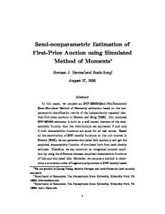
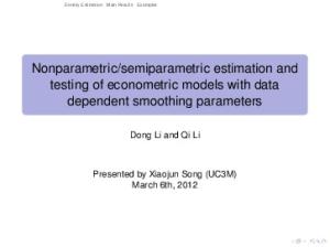
with Y1 = 0 and εi ∼ N (0, 1). The first 200 observations are dropped to eliminate initialization effects, so T = 100. The heteroskedastic regression model (1) is then estimated with the generated data. Figures 1 and 2 plot the averages, 10% quantiles and 90% quantiles (over 1000 replications) of the re-weighted local constant (RLC) conditional variance estimates at 37 equally spaced spatial points from x = −1.8 to x = 1.8, a range that is wide enough to cover most spatial points the time series visits. For comparison, corresponding results for the local constant (LC), local linear (LL) and Ziegelmann’s local exponential (LE) estimators are also plotted together with the true conditional variance function. In the two figures the smoothing bandwidths h = 0.7, 1.0 are chosen to illustrate bandwidth effects. A striking finding is that the RLC estimator has overall performance very close 11

to that of the LL estimator for all spatial points considered in terms of both bias and variability. This is not surprising given the asymptotic similarity of the methods. But in particular samples, negative LL variance estimates are found (with frequencies listed in Table 1) mainly at spatial points with sparse neighborhood or when a small bandwidth is used in which cases the estimates fluctuate widely.1 In such cases, of course, the volatility estimates are effectively useless. On the other hand, the LC and LE estimators generally suffer from large biases, especially at spatial points in whose neighborhoods there are relatively few observations, e.g. x with |x| ≥ 1. We also considered the case when the data generating process follows (10) but with scaled t(5) distributed innovations. The results are not reported here because they are similar to those given above. Figures 1-2 about here Table 1 about here

4

Empirical Applications

This Section provides two empirical examples to illustrate the usefulness of the proposed methodology. The first is a cross-section data application and the second involves financial time series.

4.1

Occupational Prestige vs. Income

Fox (2002) studied the relationship between occupational prestige and the average income of Canadian occupations2 . The data consists of cross section observations for 102 occupations. Prestige for each occupation is measured by the Pineo-Porter prestige score from a social 1

Negative local linear variance estimates are also possible for moderate or large bandwidths; c.f. Xu (2009). 2 The dataset is named as Prestige in the car package of R in Fox (2002).

12

survey. Figure 3 (a) shows the scatterplot and a local linear mean fit with the bandwidth h0 = 5809 chosen via cross validation (Li and Racine, 2004). It might also be useful to provide variance estimates for, e.g., the construction of pointwise confidence intervals for the mean or some automatic bandwidth selection criteria. Figure 3 (b) plots the squared mean regression residuals against the explanatory variable (average income) and the fitted curves that give the functional conditional variance estimates by the LC, LL and RLC methods. To clarify comparisons among these fitted curves five points with large residuals are not displayed, and the fitted curves are calculated over 186 levels of average incomes equally spaced from x = 711 to 19211. For illustration, we use the bandwidth h = 5000. It is clear that the LL variance estimates are negative at small values of average incomes, and the conventional LC estimates are always positive but suffer from large biases. The RLC estimates proposed in this paper appear to compromise very well between these two estimates, and evidently capture the declining variances in a reasonable way (being always positive) when the level of average income is low. At moderate and high average incomes the RLC variance estimates are very close to the local linear estimates, which is not surprising given their first-order asymptotic similarity. Figure 4 shows sensitivity of various functional variance estimates to the smoothing bandwidth h. We estimate the conditional variance σ 2 (x) at two levels of average income x = 1000, 6000 using 91 bandwidths equally spaced from h = 1000 to 10000. At the boundary point x = 1000, negative estimates arising from the local linear fit occur within the bandwidth range (4000, 6000), which might reasonably be chosen by empirical researchers. The RLC estimates generally lie between the LL and the conventional LC estimates, and are apparently quite stable over various bandwidths. At the interior point x = 6000, the three fitted values are much closer to each other, and the RLC and LL curves are almost indistinguishable. Figures 3-4 about here

13

4.2

Jump Diffusion Volatilities

The re-weighting idea developed in this paper can be also used to estimate for function estimation of continuous-time jump diffusions. Jump diffusion models are widely used in finance to account for discontinuities in the sample path, and are more flexible than the single-factor or multi-factor pure diffusion models in generating higher moments which match those typically observed in financial time series (see, e.g. Bakshi et al., 1997, Pan, 2002, Johannes, 2004). Our empirical application uses T = 54 years of daily secondary market quotes for 3month T-bills from January 4, 1954 to March 13, 2008, containing n = 13538 observations,3 which are plotted in Figure 5 (a). The spot rate rt is assumed to follow the jump diffusion process d log(rt ) = µ(rt )dt + σ(rt− )dWt + d

µ PIt

i=1

¶

Zi ,

where rt− = lims↑t rs , Wt is a standard Brownian motion, It is a doubly stochastic point process with stochastic intensity λ(rt ) and Zi ∼ N (0, σ 2z ). We have assumed that the mean jump size is zero without loss of generality. The four quantities of interest in estimation (the drift function µ(r), the diffusion function σ 2 (r), the jump intensity λ(r), for a interest rate level r, and the jump variance σ2z ) can be identified for a sufficiently small sampling interval ∆ by the moments Mj (r) = E(log(rt+∆ /rt )j |rt = r)/∆ for j = 1, 2, 4, 6 using the following approximate moment conditions:

M1 (r) ' µ(r), M2 (r) ' σ 2 (r) + λ(r)σ 2z , M4 (r) ' 3λ(r)σ 4z , M6 (r) ' 15λ(r)σ 6z . We use local linear fitting to estimate M1 (r), and apply the re-weighted local constant method proposed in this paper to estimate the even-order moments M2 (r), M4 (r) and 3

The dataset is available from the website http://research.stlouisfed.org/fred2 (Source: Board of Governors of the Federal Reserve System).

14

M6 (r) to avoid the occasional unreasonable negative estimates that result from local linear cj (r), j = 1, 2, 4, 6. Based on data {ri∆ , i = 1, · · · , n}, fitting. The estimates are denoted as M

following Johannes (2004) we obtain the following estimates:

σ b2z

n c c6 (ri∆ ) 1X M b = M4 (r) , , λ(r) = c4 (ri∆ ) n i=1 5M 3b σ 4z

b σ2, µ c2 (r) − λ(r)b c σ b2 (r) = M z b(r) = M1 (r).

The jump variance σ 2z is first estimated by integrating the ratio of sixth-to-fourth moments over the stationary density with the same bandwidth for the fourth and sixth moments sT −1/5 = 2.1%, where sb is the standard deviation of the sample. The estimate σ b2z h4 = 1.7b (j)

is 2.39 × 10−3 . Then, to estimate λ(r) we consider bandwidths h4 = 1.2j · h4 (j = 0, 1, 2)

c4 (r) (and therefore c4 (r). To estimate σ 2 (r) we use the bandwidth h4 in computing M in M

(j) b c2 (r), where h2 = 1.3b sT −1/5 = 1.7%. λ(r)) and bandwidths h2 = 1.2j h2 (j = 0, 1, 2) in M

j c1 (r) using the bandwidth h(j) Lastly, µ(r) is estimated by M 1 = 1.2 h1 , j = 0, 1, 2, where

sT −1/5 = 3.5%. We characterize the bandwidths used in term of the time span T h1 = 2.8b

cj (r) depend on T (or, (instead of the sample size n) since the convergence rates of the M more generally, the local time process), as shown by Bandi and Nguyen (2003), and the scale constants chosen above are such that the resulting bandwidths are close to the ones reported in empirical studies of US short rates dynamics. b The estimated curves µ b(r), λ(r), σ b2 (r) are plotted in Figure 5 (b), Figure 6 (a) and

(b), respectively. They are expected to have smaller biases than the estimates of Johannes (2004) and Bandi and Nguyen (2003), which are based on local constant estimation of the

four moments.4 Figure 6 (b) also contains the estimates (given in the higher three lines) of the total volatility function σ 2 (r) + λ(r)σ 2z . The implication is that for most short rate 4

Limit theories for the local linear and the re-weighted local constant estimators of the four moments in the jump diffusion model have not yet been available in the literature but can be studied along the line of Bandi and Nguyen (2003). For the pure diffusion models (where σ 2z = 0), the asymptotic theories for these two methods were studied by Moloche (2001), Fan and Zhang (2003) and Xu (2009).

15

levels the diffusion components explain about two thirds of the total volatility and the jump components account for about a third. This can be compared with Johannes (2004) who used a subset of our data and found that jumps typically generate more than half the volatility of interest rate changes and Eraker et al. (2003) who found that jumps in equity indices explain 10-15 percent of return volatility.

Figures 5-6 about here

5

Concluding Remarks

This paper provides a new nonparametric approach to estimating the conditional variance function based on maximization of the empirical likelihood subject to a bias-reducing moment restriction. The method is fully adaptive for the unknown mean function. The construction of the estimator does not depend on the error distribution, and it is applicable in quite general time series and cross section settings. The new estimator preserves the appealing design adaptive, bias and automatic boundary correction properties of the local linear estimator, while it is guaranteed to be non-negative in finite samples. Numerical examples suggest that the new estimator performs well in finite samples and is a promising competitor in estimating conditional variance functions. The proposed method can be extended to the case when Xt is multivariate, e.g. in the nonparametric ARCH(p) model, Yt = σ(Yt−1 , · · · , Yt−p )εt . In such cases, the constrained optimization (4) is conducted under multiple restrictions. However, the fully nonparametric volatility estimators suffer from slow convergence rates when p is large (due to curse of dimensionality effects) and difficulties of interpretation. A popular alternative that can achieve the one-dimensional convergence rate and which imposes reasonably weak assumptions on the specification of the volatility function is the additive model (Kim and Linton,

16

2004): Yt =

q α + σ 21 (Yt−1 ) + · · · + σ 2p (Yt−p )εt .

The functions σ 21 (·), · · · , σ 2p (·) can be estimated, e.g. by the method of marginal integration or backfitting, which essentially involves iterative univariate smoothing. The re-weighted local constant method proposed here is expected to be a promising alternative to the local linear estimator which is commonly recommended.

17

6

Appendix

This section provides proofs of Theorems 1 and 2. To derive the asymptotic distribution of σ b2 (x), we make the following assumptions. Assumptions (i) For a given design point x, the functions f (x) > 0, σ 2 (x) > 0, E(Y 3 |X = x) and ¨ = d2 m(z)/dz 2 and σ ¨ 2 (z) = d2 (σ 2 (z))/dz 2 are E(Y 4 |X = x) are continuous at x, and m(z) uniformly continuous on an open set containing x; (ii) E|Y |4(1+δ) < ∞ for some δ ≥ 0; (iii) There exists a constant M < ∞ such that |g1,t (y1 , y2 |x1 , x2 )| ≤ M for all t ≥ 2, where g1,t (y1 , y2 |x1 , x2 ) is the conditional density of Y1 and Yt given X1 = x1 and Xt = x2 ; (iv) The kernel functions W (·) and K(·) are symmetric density functions each with a bounded support [−1, 1]. A Lipschitz condition is satisfied by each of functions f (·), W (·) and K(·); (v) The process (Xt , Yt ) is strictly stationary and absolutely regular5 with mixing coefP 2 δ/(1+δ) (j) < ∞, where δ is the same as in (ii); ficients β(j) satisfying ∞ j=1 j β (vi). As T → ∞, h, h0 → 0 and lim inf T →∞ T h4 > 0, lim inf T →∞ T h04 > 0.

Proof of Theorem 1. The weights w bt (x) in (3) can be obtained via the Lagrange

multiplier method, viz.

w bt (x) = 5

T

1

µ

¶,

1 + λ(Xt − x)Kh (Xt − x)

See, e.g., Davidson (1994) (page 209) for the definition of an absolutely regular process.

18

(11)

where the Lagrange multiplier λ satisfies T X

(Xt − x)Kh (Xt − x) = 0. 1 + λ(Xt − x)Kh (Xt − x)

t=1

(12)

For simplicity, write the weights in the re-weighted LC estimator w bt (x) as wt in what b t ) = [m(Xt ) − m(X b t )] + σ(Xt )εt , so follows. Note that rbt = Yt − m(X rbt2

=σ

2

(Xt )ε2t

Thus by (3)

¶

µ

where

t=1

N1 =

2

σ b (x) − σ (x) =

wt K

µ

PT

Xt −x h

t=1

¶

wt K

2 N3 =

¶2

+ 2σ(Xt )εt m(Xt ) − m(X b t ) + m(Xt ) − m(X b t) 2

PT

µ

σ µ

2

(Xt )(ε2t

Xt −x h

PT

wt K

t=1

and

¶

PT

t=1

N4 =

− 1)

4 X

(14)

Nj ,

PT

wt K

µ

Xt −x h

PT

Xt −x h

wt K

¶

µ

¶

¶µ

wt K

t=1

µ

(13)

j=1

t=1

, N2 =

.

σ 2 (Xt ) − σ 2 (x) ¶ µ , Xt −x h

¶

σ(Xt )εt m(Xt ) − m(X b t) ¶ µ , PT X −x t t=1 wt K h µ

Xt −x h

PT

t=1

¶2

¶µ

wt K

b t) m(Xt ) − m(X ¶ µ

.

Xt −x h

(i). Suppose that x is such that x ± h is in the support of f (x). Since an absolutely regular time series is α−mixing, Lemma A2 in Cai (2001) holds under our assumptions, R 0 1 f (x) + Oa.s. (h3 ), where υ 2 = u2 K 2 (u)du, and i.e. λ = − hK υ2 f (x) wt = T

−1

µ

1−

hK1 f 0 (x) (Xt υ2 f (x)

¶−1

− x)Kh (Xt − x) 19

(1 + op (1)),

(15)

Consider the term N2 first. The denominator of N2 times 1/h is 1X wt K h t=1 T

µ

Xt −x h

¶

1 X = K T h t=1 T

µ

Xt −x h

¶

p

+ op (1) → f (x),

(16)

by (15) and an application of Birkhoff’s ergodic theorem (see, e.g., Shiryaev, 1996) since ¶¶ ¶ µ µ µ R 1 1 X −x u−x t = h K f (u)du → f (x) as h → 0 after a simple change of E hK h h variables. By Taylor expansion of σ 2 (Xt ) at x and the discrete moment condition (5), the numerator of N2 times 1/h is

1X wt K h t=1 T

1X = wt K h t=1 T

=

µ µ

Xt −x h

Xt −x h

¶

¶µ

σ 2 (Xt ) − σ 2 (x)

¶

1 2 ( σ ¨ (x)(Xt − x)2 + o((Xt − x)2 ) 2

h2 ¨ 2 (x) + op (h2 ), f (x)K1 σ 2

by (15) and the ergodic theorem. Combining (16) and (17) gives N2 =

(17) h2 K1 σ ¨ 2 (x) + op (h2 ). 2

Noting (15) and (16), it follows from Fan and Yao (1998, the proof of Theorem 1, (b)-(d)) ¶ µ √ d 4 (x)ξ 2 (x) K σ 2 , and N3 , N4 = op (h2 + h02 ). Hence by (14) Theorem (i) that T hN1 → N 0, f (x) holds.

(ii) and (iii). Here we only prove (ii) as (iii) can be shown similarly. Suppose that f (x) has a bounded support [a, b] and x = a + ch (0 < c < 1). By Lemma A.3 in Cai (2001), wt =

1 (1 + op (1)). T (1 − λc (Xt − a − ch)Kh (Xt − a − ch))

20

Consider the term N2 in (14) first. Note that

1X wt K h t=1 T

µ

Xt −a−ch h

¶

µ

¶

K Xt −a−ch T h 1 X p = + op (1) → K 0 f (a), T h t=1 1 − λc (Xt − a − ch)Kh (Xt − a − ch) (18)

by the ergodic theorem since

E

Ã

#

$

Xt −a−ch h 1 h 1−λc (Xt −a−ch)Kh (Xt −a−ch) K

!

=

Z

µ

→

¶

K 1 f (z)dz h 1 − λc (z − a − ch)Kh (z − a − ch)

b

a

Z

z−a−ch h

c

−1

K(u)du f (a) = K 0 f (a), 1 − λc uK(u)

as h → 0 after a change of variables. By Taylor expansion of σ2 (Xt ) at a + ch and the discrete moment condition (5),

1X wt K h t=1 T

1X = wt K h t=1 T

=

µ µ

Xt −a−ch h

Xt −a−ch h

¶

¶µ

σ 2 (Xt ) − σ 2 (a + ch)

¶

1 2 ( σ ¨ (a + ch)(Xt − a − ch)2 + o((Xt − a − ch)2 ) 2

σ 2 (a + ch) h2 K 1 f (a)¨ + op (h2 ), 2

again by the ergodic theorem. Thus, by (18) N2 =

h2 K 1 2 σ ¨ (a 2K 0

+ ch) + op (h2 ). Following the

proof of Theorem 1 in Fan and Yao (1998), it can be shown that N3 , N4 = op (h2 + h02 ) and

21

N1 is asymptotically normal with mean zero and variance 1/T h times (noting (18)) 1 2

hK 0 f 2 (a) 1

=

¶ µ ¶2 µ 2 2 X −a−ch t σ (Xt )(εt − 1) E T wt K h µ

1 K (1−λc (Xt −a−ch)Kh (Xt −a−ch))

E 2 hK 0 f 2 (a) Z cµ 1

→

2

K 0 f 2 (a)

−1

K(u) 1−λc uK(u)

¶2

µ

Xt −a−ch h

duσ 4 (a)ξ 2 (a)f (a) =

¶

¶2 σ 2 (Xt )(ε2t − 1) + op (1)

K 2 σ 4 (a)ξ 2 (a) 2

.

K 0 f (a)

So by (14) the proof of (ii) is complete.

Proof of Theorem 2. (i). We write Vb (x) = Vb1 (x) + Vb2 (x) + Vb3 (x), where

µ ¶ µ ¶ T T T X 2 X −x 4 b 2T σ b2 (x) X 2 X −x 2 b t t rbt , V2 (x) = − rbt , K K V1 (x) = h h h t=1 h t=1 µ ¶ T 4 X Tσ b (x) K 2 Xth−x . Vb3 (x) = h t=1

Consider the term Vb1 (x) first. By (13), we have rbt4

4

+ 4σ

2

(Xt )ε2t

¶2

µ

µ

¶4

3 3 b t ) + m(Xt ) − m(X b t ) + 4σ (Xt )εt · m(Xt ) − m(X ¶ ¶2 ¶3 µ µ 2 2 m(Xt ) − m(X b t ) + 2σ (Xt )εt m(Xt ) − m(X b t ) + 4σ(Xt )εt m(Xt ) − m(X b t) ,

= σ µ

(Xt )ε4t

P and denote Vb1 (x) = 6j=1 Vb1j , where Vb11 Vb12

µ ¶ T T X 2 X −x t σ 4 (Xt )ε4t , = K h h t=1 ¶2 µ ¶ µ T 4T X 2 X −x 2 2 t σ (Xt )εt m(Xt ) − m(X = K b t) h h t=1

22

¶4 µ ¶µ T T X 2 X −x b t K V13 = b t) , m(Xt ) − m(X h h t=1 ¶ µ ¶ µ T X 4T 2 3 3 K Xth−x σ (Xt )εt m(Xt ) − m(X Vb14 = b t) , h t=1 ¶2 µ ¶ µ T X 2T 2 2 2 K Xth−x σ (Xt )εt m(Xt ) − m(X , Vb15 = b t) h t=1 ¶3 µ ¶ µ T X 4T 2 and Vb16 = K Xth−x σ(Xt )εt m(Xt ) − m(X b t) . h t=1

Similar to the analysis of the term N1 in the proof of Theorem 1 (i), we have √ T µ ¶ T T X 2 X −x t √ σ 4 (Xt )(ε4t − (ξ 2 (x) + 1)) = Op (1) K h h t=1 provided that

¶ ¶2+δ/2 µ µ 2 2 4 4 X −x t σ (Xt )(εt − (ξ (x) + 1)) < ∞, E K h

which holds by assumption. Thus Vb11 = Ve11 + op (1), where T Ve11 = (ξ 2 (x) + 1) h

T X t=1

K

2

µ

Xt −x h

¶

p

σ 4 (Xt ) → (ξ 2 (x) + 1)K2 σ 4 (x)f (x)

by the ergodic theorem. It follows from Fan and Yao (1998) and the proof of Theorem 1 p (c)) that Vb1j = op (1) for j = 2, · · · , 6. Thus, Vb1 (x) → (ξ 2 (x) + 1)K2 σ 4 (x)f (x). Similarly

p p using (13) we can show that Vb2 (x) → −2K2 σ 4 (x)f (x). Lastly Vb3 (x) → K2 σ 4 (x)f (x). So p Vb (x) → ξ 2 (x)K2 σ 4 (x)f (x) and Theorem 2 (i) follows from (16).

(ii) and (iii). These can be proved as in (i) using the arguments in the proof of

Theorem 1 (ii) and (iii).

23

References Aït-Sahalia, Y., 1996, Nonparametric pricing of interest rate derivative securities. Econometrica 64, 527-560. Bakshi, G., C. Cao and Z. Chen, 1997, Empirical performance of alternative option pricing models. Journal of Finance 52, 2003-2049. Bandi, F. and T. Nguyen, 2003, On the functional estimation of jump-diffusion processes. Journal of Econometrics 116, 293-328. Bandi, F. and P.C.B. Phillips, 2003, Fully nonparametric estimation of scalar diffusion models. Econometrica 71, 241-283. Cai, Z., 2001, Weighted Nadaraya-Watson regression estimation. Statistics and Probability Letters 51, 307-318. Cai, Z., 2002, Regression quantiles for time series. Econometric Theory 18, 169-192. Chen, S.X. and Y. Qin, 2002, Confidence interval based on a local linear smoother. Scandinavian Journal of Statistics 29, 89-99. Cressie, N. and T. Read, 1984, Multinomial goodness-of-fit tests. Journal of the Royal Statistical Society B, 46, 440-464. Davidson, J., 1994, Stochastic limit theory: An introduction for econometricians. Oxford University Press, Oxford. Eraker, B., M. Johannes and N. Polson, 2003, The impact of jumps in volatility and returns. Journal of Finance 58, 1269—1300. Fan, J., 1992, Design-adaptive nonparametric regression. Journal of the American Statistical Association 87, 998-1004. Fan, J. and I. Gijbels, 1996, Local polynomial modeling and its applications. Chapman and Hall, London. Fan, J. and Q. Yao, 1998, Efficient estimation of conditional variance functions in stochastic regression. Biometrika 85, 645-660.

24

Fan, J. and C. Zhang, 2003, A re-examination of Stanton’s diffusion estimations with applications to financial model validation. Journal of American Statistical Association 98, 118-134. Fox, J., 2002, An R and S-PLUS companion to applied regression. Sage, Thousand Oaks. Gozalo, P. and O. Linton, 2000, Local nonlinear least squares: Using parametric information in nonparametric regression. Journal of Econometrics 99, 63-106. Hahn, J., P. Todd, and W. Van der Klaauw, 2001, Identification and estimation of treatment effects with a regression-discontinuity design. Econometrica 69, 201—209. Hall, P. and L.-S. Huang, 2001, Nonparametric kernel regression subject to monotonicity constraints. Annals of Statistics 29, 624-647. Hall, P. and B. Presnell, 1999, Intentionally biased bootstrap methods. Journal of the Royal Statistical Society B 61, 143-158. Hall, P., R.C.L. Wolff and Q. Yao, 1999, Methods for estimating a conditional distribution function. Journal of the American Statistical Association 94, 154-163. Hansen, B.E., 1995, Regression with nonstationary volatility. Econometrica 63, 1113-1132. Härdle, W. and A.B. Tsybakov, 1997, Local polynomial estimators of the volatility function in nonparametric autoregression. Journal of Econometrics 81, 223-242. Hjort, N.L. and M.C. Jones, 1996, Local parametric nonparametric density estimation. Annals of Statistics 24, 1619-1647. Imbens, G. W. and T. Lemieux, 2008, Regression discontinuity designs: a guide to practice, Journal of Econometrics 142, 615-635. Kim, W. and O. Linton, 2004, A local instrumental variable estimation method for generalized additive volatility models. Econometric Theory 20, 1094-1139. Li, Q. and J.S. Racine, 2004, Cross-validated local linear nonparametric regression. Statistica Sinica 14, 485-512. Johannes, M., 2004, The statistical and economic role of jumps in continuous-time interest rate models. Journal of Finance 59, 227-260. 25

Martins-Filho, C. and F. Yao, 2007, Nonparametric frontier estimation via local linear regression. Journal of Econometrics 141, 283-319. Moloche, G., 2001, Local nonparametric estimation of scalar diffusions. Unpublished paper, MIT. Owen, A., 2001, Empirical likelihood. Chapman and Hall/CRC. Pagan, A. and G. Schwert, 1990, Alternative models for conditional stock volatility. Journal of Econometrics 45, 267-290. Pagan, A.R., and Y.S. Hong (1991): .Nonparametric Estimation and the Risk Premium,. in W. Barnett, J. Powell, and G.E. Tauchen (eds.) Nonparametric and Semiparametric Methods in Econometrics and Statistics, Cambridge University Press. Pan, J., 2002, The jump-risk premia implicit in options: Evidence from an integrated time-series study, Journal of Financial Economics 63, 3-50. Porter, J., 2003, Estimation in the regression discontinuity model. Working paper, Department of Economics, University of Wisconsin. Ruppert, D., M.P. Wand, U. Holst and O. Hössjer, 1997, Local polynomial variance function estimation. Technometrics 39, 262-273. Shang, D., 2008, Robust interval forecasts of value-at-risk for nonparametric ARCH with heavy-tailed errors. Working paper, University of Wisconsin. Shiryaev, A.N., 1996, Probability. Springer-Verlag, New York. Stanton, R., 1997, A nonparametric model of term structure dynamics and the market price of interest rate risk. Journal of Finance 52, 1973-2002. Xu, K.-L., 2009, Re-weighted functional estimation of nonlinear diffusions. Forthcoming in Econometric Theory. Xu, K.-L. and P.C.B. Phillips, 2008, Adaptive estimation of autoregressive models with time-varying variances, Journal of Econometrics 142, 265-280. Yu, K. and M.C. Jones, 2004, Likelihood-based local linear estimation of the conditional variance function. Journal of the American Statistical Association 99, 139-144. 26

Ziegelmann, F.A., 2002, Nonparametric estimation of volatility functions: The local exponential estimator. Econometric Theory 18, 985-991.

27

h=0.7 3.5 LC LL

3

RLC LE 2.5 σ2(x) 2

1.5

1

0.5 −2

−1.5

−1

−0.5

0 x

0.5

1

1.5

Figure 1: The means, 10% quantiles and 90% quantiles of the local constant (LC), local linear (LL), re-weighted local constant (RLC) and local exponential (LE) estimates of the volatility function σ 2 (x) = 1 + 0.4x2 in an ARCH(1) model over 1000 replications, using the smoothing bandwidth h = 0.7.

28

2

h=1.0 LC

3

LL RLC LE

2.5 σ2(x) 2

1.5

1

0.5 −2

−1.5

−1

−0.5

0 x

0.5

1

1.5

Figure 2: The means, 10% quantiles and 90% quantiles of the local constant (LC), local linear (LL), re-weighted local constant (RLC) and local exponential (LE) estimates of the volatility function σ 2 (x) = 1 + 0.4x2 in an ARCH(1) model over 1000 replications, using the smoothing bandwidth h = 1.0.

29

2

Table 1: Frequencies of negative local linear conditional variance estimates over 1000 replications (zeros for blank cells). Bandwidth h = 0.7 h = 0.6 h = 0.5 h = 0.4 h = 0.3 h = 0.2 x = 1.8 x = 1.6 x = 1.4 x = 1.2

3

4 2

6 3

x = 1.1 x = 1.0 x = 0.9 x = 0.8

30

13 3 1

19 16 4

61 39 18 6

1

8 8 6 2

(b) Estimates of σ2(x) (h=5000)

(a) Estimates of m(x) (h’=5809) 90 80

250 Squared Residuals

70

Prestige

60 50 40

200 150 100 50

30

0

20 10 0

LL RLC LC r2

300

0.5

1

1.5 Income

2

2.5

3 4

x 10

−50 0

0.5

1 Income

1.5

2

Figure 3: Prestige vs. Income: (a) local linear estimation of the conditional mean function using the bandwidth h0 = 5809; (b) estimates of the conditional variance function based on the squared residuals using the local linear (LL), re-weighted local constant (RLC) and conventional local constant (LC) methods with the bandwidth h = 5000.

31

4

x 10

(a) Estimates of σ2(x), x=1000

(b) Estimates of σ2(x), x=6000

140 LL RLC LC

160

120 100

150

80 140 60 130

40 20

120

0 110 −20 −40

2000

4000 6000 Bandwidth h

8000

10000

100

2000

4000 6000 Bandwidth h

8000

10000

Figure 4: Prestige vs. Income: estimates of the conditional variance function over 91 bandwidths using LL, RLC and LC methods when the design point (a) x = 1000; (b) x = 6000.

32

(a)

−3

1.5

x 10

(b) h(1) 1

1

h(2) 1

15

h(3) 0 Drift Coefficient

T−bill Rate Level (Percent)

1

10

−1

5 −2

0 1955

1970

1980 Year

1990

2000 2008

−3

5

10 Interest Rate Level (Percent)

15

Figure 5: (a) The time series of daily 3-month Treasury bill rates (secondary market rates) from January 4, 1954 to March 13, 2008; (b) the local linear estimators of the drift function using three bandwidths 3.5%, 4.2% and 5.0%.

33

(a)

(b)

40

0.16 h(1) 4

h(2) 4

35

0.12 Diffusion Coefficient

30

Jump Intensity

0.14

h(3) 4

25 20 15 10

0.1 0.08 0.06 h(1) 2

0.04

h(2) 2 5

0.02

h(3) 2

0

5

10 Interest Rate Level (percent)

15

0

5

10 Interest Rate Level (percent)

15

Figure 6: (a) The re-weighted local constant estimators of the jump intensity using three c2 (r) bandwidths; (b) the re-weighted local constant estimators of the second moment M (the higher three lines) and the diffusion coefficient over three bandwidths respectively.

34