The Role of Resolution in Dasymetric Population Mapping by
Torrin Lee Hultgren B.A., Pomona College, 2000
A thesis submitted to the Faculty of the Graduate School of the University of Colorado in partial fulfillment of the requirement for the degree of Master of Arts Department of Geography 2005
This thesis entitled: The Role of Resolution in Dasymetric Population Mapping written by Torrin Lee Hultgren has been approved for the Department of Geography
________________________________________________________ Dr. Jeremy Mennis
________________________________________________________ Dr. Barbara Buttenfield
________________________________________________________ Dr. Alexander Goetz
Date_______________
The final copy of this thesis has been examined by the signatories, and we find that both the content and the form meet acceptable presentation standards of scholarly work in the above mentioned discipline.
HRC protocol # ________________
Hultgren, Torrin Lee (M.A., Geography) The Role of Resolution in Dasymetric Population Mapping Thesis directed by Dr. Jeremy Mennis The rapid pace of global urbanization is driving a demand for population maps with high spatial and temporal resolution. Dasymetric mapping is one promising method for improving existing choropleth population maps by utilizing ancillary data, such as highresolution satellite imagery classified into land-use and land-cover categories, to redistribute population counts more accurately. Traditional per-pixel classification methods tend to break down at high resolutions, however, raising the question of an appropriate pixel size for images to be classified and used in dasymetric mapping. This study used a supervised Mahalanobis distance classification of Ikonos imagery aggregated to multiple resolutions to study the role of resolution in an empirical dasymetric mapping method. It was found that while classification accuracy decreased as pixel size decreased, post-classification smoothing of high-resolution imagery achieved consistently better results than low-resolution imagery alone. The results of the dasymetric population mapping suggested that while an ideal resolution may be between 10 and 25m, the choice of empirical sampling strategy in this method has a much larger, and generally unpredictable, effect on accuracy than does the resolution or classification accuracy of the source image.
Key words: Dasymetric population mapping, resolution, urban remote sensing.
- iii -
Acknowledgements and Thanks I am deeply indebted to those who compiled and shared the data that allowed me to conduct this analysis, including the USGS, CSES, and Gary Napier at Space Imaging, whose generous donation of high-resolution Ikonos imagery truly made my work possible. Thanks also to Vanessa, Anita, and Kiyoshi who worked alongside me in the Meridian lab and empathized in times of stress and joy. My words are far too inelegant to appropriately express the gratitude I feel for those mentors who helped me in this endeavor, so I have borrowed the words of a few others. To Dr. Goetz, “A student from whom nothing is ever demanded, which he cannot do, never does all he can.”
- John Stuart Mill
Thank you for challenging me and enabling me to do more than I thought I could. To Dr. Buttenfield, "A mother is she who can take the place of all others but whose place no one else can take." - Cardinal Mermillod Thank you for taking me under your wing and giving more of your time and energy than I ever felt worthy of. To Dr. Mennis, "Be true to your work, your word, and your friend."
- Henry David Thoreau
Thank you for giving me a chance, a direction, guidance, and friendship. I am here today because of you. To Barbara, “Give in any way you can, of whatever you possess. To give is to love. To withhold is to wither. Care less for your harvest than for how it is shared, and your life will have meaning and your heart will have peace.”
- Kent Nerburn
Thank you for you. Everything is better with you, including me.
- iv -
Table of Contents Chapter 1 - Introduction ............................................................................................................ 1 Chapter 2 - Literature Review ................................................................................................... 5 2.1 - Resolution..................................................................................................................... 5 2.2 - Urban Remote Sensing ................................................................................................. 7 2.3 - Remote Sensing and Dasymetric Population Mapping .............................................. 13 Chapter 3 - Data ...................................................................................................................... 22 3.1 - Census Data ................................................................................................................ 22 3.2 - Land-Use/Land-Cover Data........................................................................................ 23 3.3 - Remote Sensing Data.................................................................................................. 31 Chapter 4 - Automated Classification of Remotely Sensed Images of Urban Areas .............. 36 4.1 - Introduction ................................................................................................................ 36 4.2 - Pilot Methods.............................................................................................................. 37 4.3 - Pilot Results................................................................................................................ 39 4.4 - Pilot Discussion .......................................................................................................... 43 4.5 - Multi-Resolution Methods.......................................................................................... 44 4.6 - Multi-Resolution Results ............................................................................................ 48 4.7 - Multi-Resolution Discussion ...................................................................................... 50 4.8 - Conclusion .................................................................................................................. 52 Chapter 5 - Writing and Testing a Raster-Based Dasymetric Mapping Script........................ 53 5.1 - Introduction ................................................................................................................ 53 5.2 - Methods ...................................................................................................................... 54 5.3 - Results ........................................................................................................................ 58 5.4 - Discussion................................................................................................................... 59 5.5 - Conclusion .................................................................................................................. 61 Chapter 6 - The Role of Pixel Size in Dasymetric Mapping ................................................... 62 6.1 - Introduction ................................................................................................................ 62 6.2 - Methods ...................................................................................................................... 62 6.3 - Results ........................................................................................................................ 68 6.4 - Discussion................................................................................................................... 75 6.5 - Conclusion .................................................................................................................. 77 Chapter 7 - Conclusion............................................................................................................ 79 References ............................................................................................................................... 82
-v-
Tables Table No.
Page
3.1
USGS Anderson Classification Schema.................................................................. 26
3.2
Seasonal Land Cover Appearance ........................................................................... 35
4.1
Accuracy Results by Classification Technique ....................................................... 39
4.2
Confusion Matrix for Smoothed Mahalanobis Distance Classification .................. 40
5.1
Processing Times for Vector and Raster Scripts ..................................................... 59
6.1
Sampling Statistics for Smoothed Data ................................................................... 72
- vi -
Figures Figure No.
Page
2.1
Example of Sensor Difficulties in Identifying Residential Areas............................ 8
2.2
VIS Model Illustration............................................................................................. 9
3.1
Image Registration with Block Shapefile Layer...................................................... 22
3.2
USGS Colorado Front Range Land-Use/Land-Cover Dataset ................................ 25
3.3
Percentile Data for Anderson Level 4 Categories ................................................... 28
3.4
Percentile Data for Aggregated Anderson Land-Cover Categories......................... 29
3.5
Percentile Data for Revised Aggregate Land-Cover Categories ............................. 29
3.6
True Color AVIRIS Image of North Boulder, CO, 10/15/02 .................................. 31
3.7
False Color High-Resolution Ikonos Imagery of North Denver, CO, 1/20/02........ 32
3.8
Laboratory Spectral Reflectance Characteristics of Common Urban Materials...... 34
4.1
Land-Use/Land-Cover Aggregations of USGS Data for Boulder Pilot Study ........ 38
4.2
AVIRIS Band Eigenvector Weights Compared with Multispectral Bands ............. 42
4.3
Ikonos Image Mahalanobis Classification Accuracy (Percent) ............................... 49
4.4
Ikonos Image Mahalanobis Classification Accuracy (Kappa) ................................ 49
5.1
Flowchart Diagram for a Dasymetric Map Using Vector Input Data...................... 54
5.2
Flowchart Diagram for a Dasymetric Map Using Raster Input Data ...................... 55
5.3
Tracts in the Denver Metro Area with the USGS LULC Dataset ........................... 57
6.1
Standard Error versus Resolution ............................................................................ 69
6.2
Misplaced Population versus Resolution................................................................. 69
6.3
Sample USGS LULC Input Data and Dasymetric Error Analysis Results ............. 70
6.4
USGS Isolated Error versus Resolution Data .......................................................... 71
6.5
Land-Use/Land-Cover Classification of Ikonos Imagery........................................ 73
6.6
Error Maps for Classified Imagery .......................................................................... 74
- vii -
Chapter 1 - Introduction The United Nations estimates that during 2000 through 2030, urban population is projected to grow at an annual rate of 1.8 percent, nearly double the rate expected for the overall population of the world. At this rate, the world’s urban population will exceed the global rural population by 2007 for the first time in history and, if the growth continues, urban population will double in just 38 years. (United Nations, 2004) This growth will be particularly rapid in urban areas of less developed regions, averaging 2.3 percent per year where resources are most limited for both measuring and coping with the growth. Although the pace of population growth is more moderate in developed countries, per capita land and resource consumption is often much greater and this sprawl can present almost as many challenges for management as population growth alone does in the developing world. In the United States, for example, growth in per capita land consumption from 1982 to 1997 actually equaled population growth at 16%. (USDA, 1997) This sprawl creates diverse headaches from school planning, infrastructure development, and water rights to destruction of habitats, pollution, and traffic nightmares. Although different in nature, in both the developed and the developing worlds the rate of urban growth is so dramatic that traditional census methods for measuring and understanding the nature of the growth are no longer sufficient. Not only are decadal intervals now too infrequent, some nations lack the financial resources to conduct a census and others grapple with bureaucratic miasmas that render large portions of census data completely unreliable (Ji et al., 2001). A need, therefore, exists to supplement traditional censuses with data that can be collected frequently, is inexpensive, and has a reliability that matches, or even exceeds, in-situ data collection. Remote sensing is emerging as a science that can already provide solutions to inexpensive yet frequent data collection but is still struggling to achieve the a high degree of -1-
reliability without tedious human editing of automated results. (Ji et al., 2001; Herold et al., 2003a; Wickham et al., 2004) One major difficulty has been the resolution of the imagery. Up until the year 1999, urban studies had to rely on Landsat (30m pixels) or SPOT (20m pixels) which were just outside of the 5-20m range that has been judged necessary to account for urban variation and complexity (Jensen and Cowen, 1999). Unlike most natural landscapes, cities are incredibly heterogeneous at all scales, often combining features such as houses, roads, trees, grass, and streams with separation of a few meters or less. Newer satellites like Space Imaging’s IKONOS (4m pixels) and DigitalGlobe’s QuickBird (2.4m pixels) have recently begun providing multispectral imagery at resolutions that should be adequate for most urban studies but higher resolution alone is not a panacea. Not only does high resolution require dramatically more storage space and processing time (making the already-expensive images even more costly) and usually comes at the expense of spectral or temporal resolution, without robust processing techniques that incorporate contextual measures, high resolution imagery has actually been shown to achieve results that are less accurate than low resolution imagery on a per-pixel basis. (Woodcock and Strahler, 1987). Thus, a need exists to understand the effects of image resolution on urban studies, and, if possible, to identify an optimum resolution. "There has... been little or no theoretical consideration of the spatial resolution (scale) of image data most appropriate to statistical or structural pattern recognition. For the first time, we have building blocks that can be assembled into objects at different scales and degrees of aggregation. This begs the question of which scale is most appropriate." (Longley, 2002) This study aims to examine the role of resolution in population mapping with remote sensing data specifically using dasymetric distribution techniques. Inclusion of the classification method in the investigation is crucial since population mapping is frequently
-2-
performed not directly with remotely sensed images but rather by using classified images to augment existing census data. This technique is one of the more commonly used methods of dasymetric mapping and it is necessary to determine whether this technique is significantly affected by the resolution of either the source imagery or the classification. Because this investigation covers a diverse range of analyses, a separate chapter is devoted to each inquiry, beginning in chapter 2 with a review of pertinent literature on resolution, urban remote sensing and its use in population mapping, and the development and refinement of dasymetric techniques. Chapter 3 gives a brief overview of the data used throughout the investigation and raises questions about the usefulness of existing landuse/land-cover categories for redistributing population data. Chapter 4 outlines a more traditional pixel-based land-use/land-cover classification methodology and examines spectral resolution requirements before conducting a full analysis of pre- and post-classification aggregation on classification accuracy. Since processing times are a serious concern with high-resolution datasets, Chapter 5 discusses the development of a raster-based dasymetric mapping tool that not only offers dramatic improvements in processing efficiency but also refines previous methods to account for challenges unique to high-resolution data. Chapter 6 details the results of this tool when put to use on the classified imagery to assess the role of resolution in dasymetric population mapping. While the results only suggest a possible ideal range of resolutions, the process uncovered important considerations related to resolution that must be taken into account both when performing and evaluating the accuracy of this dasymetric mapping technique. The goals of a high degree of reliability for automated results and identification of an ideal resolution may remain lofty but this study is expected to make important contributions. While this research alone may not exactly solve all of the problems associated with accelerated urbanization, a solid understanding of the role of resolution is necessary if urban
-3-
remote sensing and dasymetric population mapping are to make important contributions to the global understanding of urban growth.
-4-
Chapter 2 - Literature Review The literature relevant to a study of resolution in dasymetric population mapping comprises three main subject areas: the role of resolution in remote sensing and GIS in general, the current state of urban remote sensing, and the application of remote sensing to population mapping and the role of dasymetric mapping techniques. There has been significant recent research in all three areas and this chapter reviews some of the more intriguing developments.
2.1 – Resolution As this paper explores the role of resolution in dasymetric mapping, it is necessary to first explore the various aspects and ramifications of resolution in the context of GIS and remote sensing. Most people associate resolution with pixel size but spatial resolution is more aptly defined as “measure of the smallest linear separation between two objects that can be resolved” (Jensen, 2000; p.15). Aside from the use of the word itself in the definition, this meaning is much more powerful because it applies equally to both raster and vector data. It is worth noting, however, that in traditional cartography and the latest remote sensing, features smaller than the stated resolution frequently appear. On paper maps, even though resolution faces the physical constraint of about a half a millimeter, that being the smallest discernable mark to the human eye and of the cartographer’s pen, cartographers nearly always choose to include certain features smaller than scale would allow because of their semantic importance (Tobler, 1987). In remote sensing, the reverse often occurs: sub-pixel features of little importance can dominate a sensor’s response with a spuriously high spectral reflectance. The classification accuracy of a remotely sensed image has been shown to be dependent primarily on two factors, the first of which is the influence of boundary pixels.
-5-
Pixels falling along a boundary between two different classes will contain a spectral mixture of the two classes. As spatial resolution increases, the number of pixels precisely on a given boundary will decrease, resulting in fewer mixed pixels and higher classification accuracy. The second factor is the spectral variance, or “noise”, inherent to any class. As pixel size decreases and more details are resolved, this within-class variance increases, leading to lower overall classification accuracy (Woodcock and Strahler, 1987). Thus, as accuracy is a function of two competing variables, in theory there ought to be an ideal resolution for the classification of any given scene. This ideal resolution is related to the spatial autocorrelation range of the features under analysis, which can be examined using standard geostatistical methods such as the semivariogram (Bian and Butler, 1999). Because of the heterogeneity of the urban landscape, high resolution images have often been shown to have a greater percentage of misclassified pixels than coarser resolution images. However, it has also been demonstrated that when an image with resolution finer than necessary for a particular scene is aggregated to the minimum required resolution, the classification accuracy is typically better than when using images acquired at the minimum required resolution (Cushnie, 1987; Woodcock and Strahler, 1987). Although this can be due to a number of reasons, it is generally a result of the highly controlled nature of the postacquisition focal map algebra aggregation as opposed to the more complex, and potentially unpredictable, sensor response functions, particularly with regard to spurious sub-pixel reflectors. Post-classification aggregation can be even more powerful in that it is biased specifically toward relevant and meaningful categories (Saura, 2002). In the context of population mapping using ancillary data, the same relationship between resolution and accuracy ought to hold true. It has been suggested that regional population estimation can be effectively performed at spatial resolutions of 5m to 20m (Jensen and Cowen, 1999). Others have speculated that as pixels are reduced to excessively small sizes in dasymetric mapping, the overall map error would increase (Eicher and Brewer,
-6-
2001). Although it may be inappropriate to study population distribution at a resolution of 4m and pixels of that resolution may lead to increased map error, data aggregated after classification ought to be more accurate than data aggregated prior to classification. This study examines not only the classification accuracy of images degraded to a range of resolutions from 4m to 48m, it also compares the population distribution accuracy of those images aggregated prior to the classification with data at the same range of scales aggregated after classification.
2.2 – Urban Remote Sensing The field of urban remote sensing, while still relatively new compared to other remote sensing specialty areas, is nevertheless exceedingly broad and burgeoning – aptly reflecting not only the complexity of the landscape itself but the diverse nature of the interests and concerns of city managers and urban geographers. Several notable journals in remote sensing have recognized the growing importance and relevance of urban remote sensing and have chosen to devote entire issues to the subject. These include the International Journal of Remote Sensing in February 2005, Photogrammetric Engineering and Remote Sensing in September 2003, Remote Sensing of Environment in August 2003, IEEE Transactions on Geoscience and Remote Sensing in September 2003, and the June 2003 issue of the ISPRS Journal of Photogrammetry and Remote Sensing. A review of all of this state-of-the-art literature in urban remote sensing is unfortunately beyond the scope of this paper. Instead, a brief summary of the nature and concerns of urban remote sensing is outlined, followed by a discussion of traditional per-pixel classification techniques and the trends toward contextual classification methods that has occurred since the advent of high-resolution imagery.
-7-
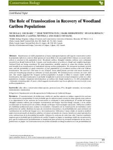
The challenges facing urban remote sensors are due to the complexity of cities themselves. The simple question of where the countryside ends and the city begins is difficult enough to pin down semantically, so it’s no wonder that developing reliable rules and techniques for defining extent in terms of spectral characteristics, patterns, and textures is even more taxing. Urban features can be highly irregular, urbanization density can vary continuously (Clapham, 2003) and change abruptly (Turpin and Roux, 2003), actual urbanized areas can differ greatly from official administrative boundaries (Wilson et al., 2003), and many areas within a city limits (such as city parks) can be, or merely appear to be (see Figure 2.1), exactly like the countryside. Also, the same processes or algorithms that are used to separate urban areas from surrounding forests may not be effective for cities in a desert environment (Ridd, 1995), or even the same city at different times of year (O'Hara et al., 2003). Still, a great deal of current research focuses on developing, refining,
Figure 2.1: Both areas appear to a remote sensor as wooded. (Clapham, 2003)
and automating these processes and algorithms for further research use (Ward et al., 2000; Herold et al., 2003b; Segl et al., 2003; Shackelford et al., 2003; Yang et al., 2003; Zha et al., 2003; Herold et al., 2004; Wu, 2004). One study in recent literature seems to embody many of the motivations, goals, and difficulties of urban remote sensing. C. Y. Ji, et al. (2001) detail a large project in China to study urban extent and built-up areas using remote sensing. Apparently in China, local land use and population statistics are frequently compromised by local officials changing figures and falsifying maps when reporting up through the bureaucracy. Clearly the central
-8-
government would like to use remote sensing as a third-party verification to keep such manipulation and/or falsification in check. The primary project goal, therefore, was to produce accurate maps of land cover for over 100 cities in China with the evaluation of various classification techniques as a secondary objective. They were able to accomplish the primary goal and managed to identify a number of illegal developments as well as critical areas of arable land under pressure from development. However, in order to achieve at least 90% classification accuracy for the final maps, extensive manual post-processing of all of the automatically classified images was required. The average accuracy for the automated classification was around 80%, despite the fact that very broad classes were used (i.e. Urban Features, Arable Land, Forest & Orchard, Grassland & Pasture, Barren Land, Open Water Surface, and Development). These categories are very similar to those used in this investigation into resolution in dasymetric mapping, with slightly fewer natural classes and an aspiration for additional urban classes. This research, however, is less concerned with overall accuracy and more with the relative accuracy of automated classification at various scales. Traditionally, remote sensing has focused on classifying images on a pixel-by-pixel basis using their spectral signature. This assumes that the reflectance measured in each pixel is a linear combination of various spectrally pure
Figure 2.2: VIS Model Illustration (Ridd, 1995)
“end members.” The VIS (Vegetation-ImperviousSoil) model is a well established example of this technique (Figure 2.2). The theory is that healthy vegetation, bare concrete,
-9-
and bare soil are the primary contributors to a pixel’s spectral signature and the actual makeup of the pixel can be inferred from the proportions of each (Ridd, 1995). This model has proven to be quite reliable in a wide variety of urban environments and continues to be used with medium to low resolution (30-100m) imagery (Wu, 2004). Still, at these lower resolutions, the overall accuracy of automated land-cover classification projects such as the National Land-Cover Dataset (NLCD) has been shown to be discouragingly low for Anderson Level II classes (A full discussion of the Anderson Land-Use/Land-Cover classification hierarchy can be found in Chapter 3) – only 38% to 70% accuracy across regions of the western United States (Wickham et al., 2004). One of the assumptions which the dasymetric technique used in this paper is based upon is that there is a distinction between at least two different residential ancillary classes. Since a division in residential classes does not occur until Level III of the Anderson hierarchy, more refined techniques and better resolution are clearly necessary to study residential density. One possible alternative to higher spatial resolution that is considered in this paper is increasing spectral resolution, usually referred to as hyperspectral sensing. The concept behind hyperspectral sensing is that because the electromagnetic spectrum is continuous, a sensor that collects data in very narrow sequential bands across the entire spectrum is better suited to distinguishing materials spectrally than a typical multispectral sensor that uses only a limited number of broad spectral bands. While this extremely fine spectral resolution (hundreds of bands 0.01µm wide versus seven band 0.1-0.2 µm wide) may not be necessary for all remote sensing applications, the sheer spectral complexity of the urban environment suggests that a hyperspectral approach may be warranted. Herold et al. (2003) used AVIRIS spectral imagery and a spectral library of urban surfaces gathered in situ in the Santa Barbara area to attempt a classification of 26 separate land cover classes and to identify those ‘ideal’ AVIRIS bands that demonstrated the most
- 10 -
‘separability’ for the images. The classification was performed both with those ‘ideal’ hyperspectral bands as well as with those bands that, when combined, corresponded to the Ikonos and Landsat TM multispectral bands for comparative purposes. While the AVIRIS ‘ideal’ bands performed significantly better than the simulated Ikonos (37.0%) or Landsat (53.9%) images, overall classification accuracy did not exceed 66.6% for the 22 urban classes, largely due to spectral similarity between different land cover classes as well as significant within-class variation. Another study with fewer spectral classes was focused specifically on comparing Landsat and AVIRIS data and, similarly, concluded that increased spectral resolution alone (although interestingly not a higher signal to noise ratio (SNR)) can improve classification of almost all land-cover types (Platt and Goetz, 2004). The study suggests that while urban classification may not be achieved using spectral information alone, hyperspectral imagery and comprehensive spectral libraries can be much more accurate than multispectral sensors in an urban environment. The identification of those bands with the most surface ‘separability’ in urban environments of interest could potentially influence the selection of the next generation of multispectral sensors. In all likeliness, however, every different city in the world would recommend a slightly different set of ideal bands, suggesting that the next generation of remote sensors should simply all be hyperspectral! Nevertheless, in any one image there is a limit to the number of spectral “dimensions”, that is, regions of the spectrum that contain non-redundant information. As such, further improvements in automated urban classification will have to either include textural or contextual information or utilize other types of data to generate truly useful data. Chapter 4 includes an analysis of the spectral bands with the greatest variance in the Front Range area of Colorado and while the bulk of the research used imagery with very limited spectral resolution, if automated remote sensing is going to make
- 11 -
reliable contributions to population mapping, a combination of high spatial and spectral resolution may be necessary. Recent improvements in the resolution of satellite imagery have offered researchers the opportunity to improve upon poor automated classification performance. High resolution itself is not a panacea, however, because decreasing pixel size has the effect of dramatically increasing the number of distinct spectral signatures and thus the spectral variance within (and in many cases the similarity between) distinct semantic classes (Herold et al., 2003a). Individual pixels are no longer linear combinations of end members that can be predictably placed into classes. Instead, traditional classes are a jumble of many spectrally distinct pixels. This is particularly true in urban residential settings where trees, lawns, rooftops, and pavement intermingle in an endless variety of patterns. Without taking into account this context, it would be impossible to distinguish a tree in a yard, that should be classified as residential, from a tree in the middle of a forest that should be classified as natural vegetation. Traditional photointerpretation utilizes the incredible capacity of human cognition for identifying contextual traits to understand scenes. These traits include texture, shape, shadow, size, relative location, and spatial pattern. In order to incorporate context into remote sensing classification, researchers have begun to examine textural and contextual metrics that quantify the patterns in urban imagery (Liu, 2004; Pesaresi, 2000). It has also been found helpful to study these patterns at a number of different scales, due to the significant heterogeneity of urban environments at multiple scales (Karathanassi, 2000). Herold et al. (2003a) explored the use of texture algorithms such as local pixel uniformity, variance, and contrast with spatial metrics such as patch size, patch density, and fractal dimension of patch borders. Although far from being practically robust, the success of the combination of techniques in this study, as well as the shape analysis by Segl et al. (2003), appear promising but studies on textural analysis of high- (and in the future very high-)
- 12 -
resolution imagery remain at the forefront of urban remote sensing research (Puissant et al., 2005). Yet even these recent developments in textural analysis and high resolution shape recognition face fundamental limits because of the often tenuous relationship between any parameter visible from space and the actual land use to be inferred from that parameter. Some even go so far as to say that in an urban context “further progress will eventually require that spectral land cover data be supplemented with ancillary information (e.g., landuse geometry or population size) if more plausible classifications of land use are to be created.” (Longley, 2002) While some purists balk at the reliance on outside sources of information of potentially dubious accuracy, it may well be that such methodologies eventually will become standardized. The use of population geodemographics to guide and refine the classification process is becoming more commonplace (Abed and Kaysi, 2003; Harris, 2003) and studies that utilize multiple data sources may represent the future of urban remote sensing image analysis. In fact, the refined population maps this study aims to produce could themselves be used to increase remote sensing classification accuracy, creating a feedback loop of continually improving results. Care must be taken, however, that this loop does not cause error propagation of unintended effects.
2.3 – Remote Sensing and Dasymetric Population Mapping The discussions above have focused on more general studies of resolution and urban remote sensing. This last section of literature review, however, is specifically focused on population mapping which is the core of this project. First, studies that try to infer population distribution directly from remotely sensed imagery will be surveyed, followed by several studies that redistribute census counts without the use of any ancillary data. Lastly, and in the spirit of data integration mentioned at the end of the last section, the review will cover
- 13 -
techniques like dasymetric mapping that combine remote sensing imagery with census data to achieve some of the most accurate population maps available. Night-time imagery, while of coarse 1km2 resolution and limited accuracy for actual areal measurements, has nevertheless been shown to be reasonably reliable for large-scale population estimation. It offers the additional appeal of a small dataset size, high temporal resolution, and the simplicity of a single variable that is almost exclusively anthropogenic. Sutton (2003) explored the use of night-time imagery for national and international population estimates. He found a significant log/log correlation between light cluster area and metropolitan population in the United States, and in general, for cities at similar levels of economic development. Although the relationship tended to decay with smaller populations and smaller areas, by weighting larger cities, he was able to attain an R2 value of 0.98 (1,383 sample points) for the U.S. A similar regression was developed for every nation based on those cities with a known population and an estimate of global population was thereby established. The accuracy of those national estimates as compared to the USGS International Geosphere-Biosphere Program estimates did vary widely but they were within 25% for 65% of the most populous nations and the global estimate was only off by 7%. Since the compounded uncertainty of any estimate of global population is likely to be of a similar magnitude, it is possible that Dr. Sutton’s estimate is as close to the actual global population as conventional estimates. With some refinement of spatial accuracy and calibration of light intensity levels across various levels of economic development, night-time imagery may merit serious consideration for intracensal estimates on a national or regional basis. The disadvantage, however, is that at higher resolutions, brightly lit uninhabited areas such as parking lots and car dealerships or older residential neighborhoods with dense canopies that dampen light transmission tend to break down the reliable correlation between light intensity, persistence, and population density.
- 14 -
Most demographic studies using remote sensing require much finer measurements. Pozzi and Small (2002) attempted to establish a reliable relationship between vegetation and population density at 30m Landsat resolution and the poor results suggested the need to explore spectral heterogeneity at multiple pixel scales and possibly including ancillary data to augment the analysis. Lo (2003) attempted to develop a statistical correlation between urban census tract population and the area within each tract that had been classified as residential from Landsat imagery. Unfortunately, urban population density can be extremely variable and even dividing up the tracts into regions of high and low density development failed to produce accuracy of better than 85% using an allometric (logarithmic) model. The equations tended to overestimate population in the urban periphery, where both the tracts and the areas classified as residential were very large, and underestimate population in the urban core where small census tracts hold a very large number of people in tall buildings. This suggests that until remote sensing can incorporate three-dimensional information about buildings, even high resolution satellite imagery may be of limited use for estimating census tract population. One of the ways to incorporate three-dimensional information is to use radar images which are highly sensitive to building geometry. Although radar images are often challenging to interpret, and thereby relate to demographic variables, Hall et al. (2001) found an intriguing connection between certain radar signatures and pockets of urban poverty in Rosario, Argentina. This particular backscatter signature was related to the housing materials unique to squatters’ villages in this area, meaning the results would be difficult to replicate anywhere else. This study highlights that demographic variables are critical and must somehow be related to consistent physical parameters if they are to be studied by remote sensing. On the other hand, specific urban physical parameters can sometimes represent such a barrier to remote sensing that certain areas are simply excluded from study. For example, Qiu et al. (2003) developed a model for estimating population growth based on uniform
- 15 -
population per pixel classified as urban in the Dallas, TX area. This methodology was fairly accurate over the study area because most of the growth was occurring with a consistent population density. However, both high density urban areas and older neighborhoods with extensive tree cover, which are extremely common in U.S. cities, were excluded from the study because of their ability to confuse the model and weaken the correlation, once again demonstrating the difficulties of a purely remote sensing method. So if a purely remote sensing method is not the answer, why not stick with census data that is already known to be reliable? Most censuses will only publish demographic statistics that have been aggregated across certain areas, foremost for obvious privacy reasons, but also because the nearly constant change at the housing-unit level makes ensuring the accuracy of finer resolution data nearly impossible. The challenges that grouping census data into enumeration units create, however, are numerous and formidable. In outlining boundaries, a census attempts to form areas that are relatively homogenous in terms of demographic characteristics (socioeconomic, racial, and housing type) at the time of establishment, as well as approximately equal in population (U.S. Census, 2001). In order to keep total population approximately consistent in each unit, the units are undoubtedly inconsistent in area. While these units can be quite functional for certain studies, the assumption of population homogeneity across often very large and arbitrary areas can be both misleading and erroneous. Numerous methods have been explored to redistribute census counts. Some researchers have employed interpolation techniques to develop a population surface based on weighted distance from tract centroids (Bracken, 1993; Harris and Longley, 2000; Harvey, 2003). Richard Harris (2003) used a centroid decay model in Bristol, England, to try and address the problem mentioned above of areas that are classified as urban but contain little to no actual residents. U.K. postcodes, which are divided into residential and commercial, define small groups of neighboring mail delivery points. Although the areas that a postcode
- 16 -
represents are amorphous, software programs are available that assign a centroid to each that roughly approximates the geographic center according to the list of properties. A distance decay function of population probability from the center of the residential postcodes can aid in eliminating population from areas that are heavily commercial or industrial, or in the case of Bristol, on the M32 motorway that had also been prominently classified as urban. This technique would probably be less successful in the U.S., where census blocks are not divided into commercial and residential areas and are often irregularly shaped to maximize resident homogeneity. Alternatively, as Harvey (2003) demonstrated, a raster density surface with decreasing population per pixel and increasing distance from the city center could be applied to increase the robustness of the land cover model. The difficulty lies in determining the appropriate form of the regression function in the face of often nonlinear, or even chaotic, urban population distributions as well as an appropriate way to account for areas that appear urbanized but actually contain a very low population, such as airports and industrial facilities (even though during the day these areas may actually have far more people than residential areas – calling into question the convention of locating people according to where they sleep). Additionally, any decay function relies on an assumption about urban morphology and districting choices rather than a measurable parameter. While this method does create maps of some utility, it is based on several assumptions that, upon further inspection, appear shaky. For instance, the assumption that population will decay in any sort of predictable fashion with decreasing distance from a centroid or cluster of centroids might be confounded by, say, the clustering of population along a waterfront at the very edge of an enumeration district. In our study area of Denver, Colorado, the Platte River corridor is a good example of this phenomenon. Although the river itself is meager by most standards, a transportation corridor developed alongside it that cuts a wide swath of zero population through some of the most densely populated areas in the city. Corrections for such exceptions to the predictability of population-decay theory have to
- 17 -
be handled manually on a district-by-district basis, based on first-hand knowledge of the area, which is a labor intensive process. As the relative ease and resolution of remotely sensed urban classification continue to increase, methodology should, ideally, switch from such models and assumptions to actual measurements that account for the true heterogeneity of the urban environment. Qui et al. (2003) performed a population growth estimate based on assigning new population according to the length of new roads obtained from US Census TIGER GIS data. This provided them with even better accuracy than their remote sensing study discussed above. Hawley and Moellering (2005) achieved similar results, demonstrating the effectiveness of basing population estimates on lengths of road in an areal unit. This suggests that current research efforts to derive street centerline maps from remotely sensed images, rather than GPS data, might be able to contribute to population estimates as well. One might even explore the relationship between population growth and arterial road width or total road surface area given this type of data. With GPS devices today, mapping lengths of new road is almost always easier than obtaining satellite photos of the same area. Still, the GPS method is not fallible and cannot account for changes in population density that occur without changes to road length where remote sensing methods might be more sensitive. “If remote sensing data are integrated or used in conjunction with other sources of socioeconomic, administrative, and regulatory data, their potential applicability to both research and policy understanding of the urban environment increases significantly.” (Miller et al., 2003). To reduce labor and reliance on uncertain assumptions, researchers have looked to incorporate ancillary sources of data on which to create more accurate population maps. Utilizing discrete categories derived from an ancillary dataset to redistribute population within broad (and often arbitrary) enumeration units is one example of a more general technique in thematic cartography known as dasymetric mapping. Dasymetric mapping is more precisely defined as the portrayal of “a statistical surface as a series of zones of uniform
- 18 -
statistical value separated by escarpments of rapid change in value.” (McCleary, 1969) The advantage this method offers is that “it provides for abrupt changes of density which often are very real on the ground.” (International Geographical Union, 1952) A dasymetric map was first created in the 1830s and Russian cartographers gave the concept a name in the 1930s (from the Greek, meaning “Density-measuring”) but although there has been general agreement over the purpose of a dasymetric map as defined above, there is certainly not a consensus for a preferred means to the end (McCleary, 1969). Even J.K. Wright’s (1936) paper, which some regard as the seminal dasymetric mapping work for American geographers, used a method no more standardized than what Wright himself termed “controlled guesswork” (Wright, 1936). Recent advancements in geographic information systems, as well as the increased availability of digital datasets, have revitalized the concept. Yet despite the renewed interest, dasymetric mapping still lacks a standardized methodology and, as a science, has not progressed very far beyond simple automation. Purely defined, the dasymetric method does not require ancillary data upon which to base population distribution. For example, if one had population data that identified the precise location of every single person in an area, one might generate an accurate dasymetric map on the basis of that data alone. In the absence of such data, however, cartographers have turned to a wide variety of ancillary datasets to solve the problem of arbitrary choropleth enumeration units. Some of the more frequently used ancillary datasets are land-cover maps, such as those produced via satellite imagery. With various land-cover classes, however, the key question becomes how to distribute the population among those classes. The most basic technique is known as binary classification, wherein all classes are designated as either inhabited or uninhabited and the population is distributed by areal weighting into the inhabited areas of each enumeration district. This simple method has been shown to improve areal interpolation accuracy by almost 33% over choropleth mapping (Langford, 2003), although further refinement is most certainly warranted.
- 19 -
Suggested methods for improvement include: a density regression for the different land covers, field sampled density values, or a standardized set of density fractions to apply to all districts as a distribution method or a limiting variable. The latter option might, for example, involve distributing 80% of district population into any built-up areas, 15% into agricultural areas, and 5% to other land covers excluding bodies of water (Donnay and Unwin, 2001; Eicher and Brewer, 2001). All of these methods are flawed in some way, though. A density regression can predict negative population densities and is apparently quite sensitive to classification error. Field sampling of density is time-consuming, expensive, and challenging. And clearly no standardized ratios will be appropriate for all study areas, making density fractions reliant on potentially dubious assumptions. What seems to be called for is a distribution technique that mines the available data to make decisions about class distributions. XiaoHang Liu (2003) presented a novel approach for population mapping that combines the smoothness of an interpolation model with the acuity of remotely sensed imagery. In this method, homogenous urban patches (HUPs) are designated based on the land use and image texture and an expected population estimate for each patch is assigned using a regression on the image texture parameters. To further refine the accuracy, census units are then identified that lie fully within an HUP (which is assumed to have homogenous population density in addition to texture and land-cover parameters) and the difference between the estimated and actual population for these areas are used as the source points for a co-kriging model. This model assigns a residual value (which may be positive or negative) to each HUP such that the pycnophylactic integrity of larger census units is preserved. The use of homogenous patches defined from urban imagery is definitely a method that many remote sensing researchers are looking to, although the tools and techniques for doing so are still in their infancy.
- 20 -
Mennis (2003) proposed a similar solution that mines ancillary data for population estimates and can be more easily performed using existing software and data. Population density values for each ancillary class are calculated based upon the total density of all census source units that lie entirely within that class. These values can be calculated across the entire study area or different relative ratios can be calculated for smaller areas, such as census tracts. This avoids potentially fallacious assumptions and customizes the dasymetric distribution using the population values that one is already assuming are reliable. Trusty (2004) applied this technique to redistribute block-group populations in Alameda County, CA, and achieved correlation coefficients with block level population as high as 0.88. One difficulty that this initial method faced, however, is that as the spatial resolution of the remotely sensed land cover areas improves, it will become increasingly difficult to find even block groups that lie entirely within one land cover type. In this research project, the selection technique was modified by designating block groups as representative of a land cover type if that land cover comprised a certain percentage of the total block group area, i.e. 90-95%. This refinement should function at all levels of spatial resolution and can be easily performed using existing GIS techniques (as shown in Chapter 5), though the sheer number of steps and intermediate values involved in the calculation, as well as the need for repetition to determine the ideal sampling threshold, have suggested the benefits of automating this procedure. One might argue that dasymetric mapping represents an ideal synthesis of remotely sensed information and more traditional geodemographic data. A robust, highly accurate dasymetric map could have a number of potential applications, from growth modeling and traffic analysis to environmental impact studies and disaster management. A thorough analysis of the role of resolution in dasymetric mapping is one more step towards making this technique practical and reliable in a wide range of global contexts.
- 21 -
Chapter 3 - Data This research utilizes primarily three datasets for the Colorado Front Range for different analyses, as well as a fourth image for a single study. Rather than introduce the datasets as they are first used, it seems more efficient to present them up front. The data are U.S. Census blocks data, an Anderson-style land-use/land-cover dataset, a high-resolution Ikonos satellite image, and a hyperspectral AVIRIS image.
3.1 - Census Data A boundary file of census blocks for the state of Colorado in the year 2000 was the primary census dataset. The data were a resource available from the University of Colorado Department of Geography. Although metadata was not attached to the dataset, it was assumed that the block boundary file was derived directly from the US Census Bureau TIGER database, with the standard coordinate tolerance of 0.0003 decimal degrees, which is equal to approximately 30m in the study area. This low tolerance for coordinate accuracy is evident in the
Figure 3.1: The green circles indicate vertices that are approximately at the exact center of their respective intersection on the image. The red circles indicate intersections that deviate from their location on the image by more than three pixels. This illustrates that although there are no systematic registration errors (that is, one dataset is consistently shifted to the right, for example) the block shapefile does contain a significant amount of variance in the registration accuracy of individual vertices. - 22 -
data and may have made a non-negligible contribution to the overall error of the analysis. Although the blocks layer was georegistered relatively well with the imagery, block boundaries that seemed like they should be following street centerlines appeared in many places to zigzag back and forth across the street (Figure 3.1). It is unclear precisely how this may have influenced the final results, for the deviation never appeared to be more than a few pixels in either direction and the errors seemed to be randomly distributed. More information about census boundary files is available at: http://www.census.gov/geo/www/cob/scale.html. (Last checked 2/26/05). The blocks were checked for topological consistency and population count data was downloaded from the census website and attached to the attribute table. To ensure that the blocks nested perfectly within the tracts, a census tract shapefile was derived from the blocks shapefile using the Dissolve tool in ArcGIS 8.3. Due to the generalization algorithms the census uses to reduce file size for data made available to the public, units are not necessarily vertically integrated across resolutions. The counts, however, should be consistent regardless of the condition of the boundary files and this was verified by comparing the population counts for the aggregated blocks with the count tables for the tracts.
3.2 - Land-Use/Land-Cover Data A high-resolution land-use/land-cover dataset was generated in 1996/97 through manual photointerpretation of a combination of 1m airborne and satellite imagery by the USGS as part of the Land Characterization research activities for the Front Range Infrastructure Resources (FRIR) Project. Although one might be able to consider the nominal point accuracy of the dataset as ±1m, this accuracy applies only to the points and lines forming the boundaries of the polygons. The land cover polygons themselves, however, have a minimum mapping unit (MMU) size of approximately 2.5 acres (10,100 m2), with a minimum width of 125 feet (38.1m). Unique land-cover units smaller than the MMU were simply subsumed into similar adjacent units at the discretion of the individual - 23 -
photointerpreter. Thus, for this dataset, there are actually two types of spatial resolution: point accuracy and MMU size, a critical, and often confusing, distinction. The data is available to the public at: http://rockyweb.cr.usgs.gov/frontrange/datasets.htm in ArcInfo Coverage format. The availability of such a high-resolution, high accuracy land-use/landcover dataset is unique and although the temporal asynchrony with the census and image data was problematic given the rate of sprawl in the study area, a comparable dataset was not readily available. An illustration showing the extent and context of the dataset with classes aggregated for this research is shown in Figure 3.2. One type of resolution not discussed in the literature review above is known as categorical resolution and it is particularly relevant for this dataset, which uses a modified Anderson hierarchical land-use/land-cover classification. This schema was developed as a classification system specifically for remotely sensed data and each level of the hierarchy was intended to represent the distinguishable classes at increasing resolutions (Anderson et al., 1976 – See Table 3.1 for an example). One of the fundamental assumptions of dasymetric mapping is that an ancillary dataset contains information that is somehow relevant to population distribution. Mennis (2003) proposed a distribution technique that, first, assumes that the ancillary data contains classes that are relatively homogenous with respect to population density and, secondly, mines the available data to make decisions about class distributions. Thus, for this method, it is more important to have classes that minimize internal variance (at least within the confines of a particular study area) than to have classes that precisely predict population density. In theory, an Anderson Land Cover classification schema ought to be able to provide such categories that are both distinguishable in remotely sensed images and relevant for population mapping. This researcher’s own prior experiments have demonstrated the feasibility of using remotely sensed imagery to map land cover in an Anderson level schema with a reasonable degree of accuracy. This is discussed in greater detail in Chapter 4.
- 24 -
Additional exploration has also shown the effectiveness of this particular dasymetric mapping methodology as compared to previous methods but overall accuracy was impeded by apparently large variances in many of the chosen classes, which had been created as
Figure 3.2: Extent and Context of the USGS Colorado Front Range Land-Use/Land-Cover Dataset. Classes shown are those aggregated for this research. - 25 -
aggregations of semantically similar categories in a slightly modified Anderson schema. Before progressing further with this research it therefore appeared necessary to examine the population density variance in each of the classes at the finest level of categorical granularity of the dataset in order to achieve more effective groupings. A table illustrating the USGS modified Anderson Schema for this dataset is shown below. The original grouping was made by trying to subdivide the existing hierarchy as little as possible, as those categories had supposedly been developed with remote sensing research in mind. Thus, “Developed” was the only Level 1 category subdivided to get residential Table 3.1 – USGS Anderson Classification Schema
- 26 -
classes. After the initial analysis, however, the categories were regrouped to maximize class homogeneity with respect to population density. The revised groupings are also shown in Table 3.1. To aid the remote sensing classification portion of the analysis, the vegetation category was divided into irrigated and natural vegetation, as the spectral difference between those categories in the arid high-plains landscape is substantial. Irrigated vegetation classes are shown in the table in a darker shade of green. This distinction, however, was not carried over into the population portion of the study, as neither vegetation class was expected to be populated. Although High Density Residential in particular was expected to be difficult to separate spectrally, with high spectral variance and many similarities to Low Intensity Residential and Commercial/Industrial, the distinction was deemed important enough to population studies that it remained throughout the study. In order to measure the population density variance, an intersection was performed using the census block map and the land cover dataset. Since blocks are the smallest geographic entities for which the U.S. Census Bureau presents data, it was assumed that each block had homogenous population density (a discussion concerning the limits of this assumption can be found in Chapter 6). Assuming uniform density allowed population distribution by areal weighting – that is, for any block that was subdivided by multiple land cover types, population was distributed into the subdivisions by multiplying the density of the source block by the area of the internally created polygons. Once the population of all of the intersected polygons was estimated in this manner, the data were re-aggregated back to the initial land-cover units, resulting in a total population and density value for each of the landcover polygons. Summary statistics were then calculated for each land-cover category: mean density, 5, 25, 75, and 95 percentiles, and total population. The latter value was divided by total class area to calculate a total class density for comparison with mean density. Charts illustrating these values for both the semantically aggregated and all of the individual classes are included as Figures 3.3, 3.4, and 3.5.
- 27 -
- 28 -
0
1000
2000
3000
4000
5000
6000
7000
The shaded areas represent the traditional boxplot boundaries: the 25th and 75th percentiles for Mean Density, which is the unweighted mean of all records/rows/polygons of that land cover category. The whiskers extend to the 5th and 95th percentiles. They are ranked, however, according to total density, which is the total population divided by the total area for the entire class. Total class population is also shown to identify the relative importance of the classes.
Total Density Mean Density Total Pop
Percentile Data for Anderson Level 4 Land Cover Categories
s l l l al s l s y n t y d y s il h n s y s s n d al r r ts s n e s s d s s d e s d s oi Pi nd ve te str nd an tio and or ody lat te tur ped sa er tia nti ba pe nti ice ol na fice na rk itch se str ta itc tio rie itch tio iliti es nd nd ve str ve ou are te ou en ide Ur elo ide erv cho sitio Of utio Pa l/D our ndu Re l/D rea ete l/D rta Ut sin tla tla Gro du Gro ce - B tiva ce erv vel tla /Ri ltiva du /Po /S era ubl Airp o - F res cul elo spo efin d k p l r n a i R / i s e m u n s/ W t a es ra e - tit an o u e v e I r t o a a I c a I s d v S a & S c n s u s C o b b m k p t D e t j h n n F - ra n ns rb e Re ixe D Re & a an /Re Ce an ns ns al B y W - W ard ght rd er de /C er - R /G an olf gh t W trea d/C avy La Ro g O - S ent ral ide l - Aqu De t - ical e I U i ya l H si ed H r s en - R ily - e in M ial ily tail n e a l - d C ra tio ur od te ey u ity - T id s e d - M d C nt - C G /Li - L ine ra Re ant al - ate ine rg r - S ant - H ter ar ed ura esi at Re tur nt - ent ide em o iga in ity am ity - ent am Re ens ity Res ent te - ter te - ial nt ine me ate ine - T ica cult t e l B u h N s a l r t e t W a t e V c M l r n f f i V n W ip te P nt W t - F Na -R g_ on _N ide sid Res o-c m en lti- ens esid le- nor w-D ens on- sid riga Wa iga er sid Un tai Irrig - L en un gr e - _Ir ds/ ide ds/ Na on - P atu a n N al tr - E W ted ide -D Mu -D -r ing Mi N en ined g_ No Ve N eg Res -Re on- etr o -D N -Re _Ir Irr mm -Re r - ter g_ ter sid mm t - A gat eg har es har al S r h _ d s a e / L i n _ e / V t f e P n n a o V rc u g i e w h o -S d g ig N g Co on ate E a V -R rc ur es on Veg es on Ve W n-R - C den _Irr at Ve e H ity Hig - N rri -R on No t Lo O N Ve t rri rrig N on O at ix i N W nt N y -R C - I on t s o g en d N e - _N n ua g_I g_ nt nsit - M N en Res Ve e on nt N id te en te e t e e d Q g s d a a d i N i na e e i V e e id De ity -D g s g s i g s i V s i d t h r V e i e e o rr -R e s Ir ig Irr en -R es -R N -I -R H -R Low en on g_ id R g_ e on N on on on -D nes N Ve at N N Ve N w o g R i N Lo Irr on g_ N Ve
Population Density (people per square km)
8000
Figure 3.3
Figure 3.4 Percentile Data for Aggregated Anderson Land Cover Categories 8000
Total Density Mean Density Total Population
Population Density (people per square km)
7000
6000
The shaded areas represent the traditional boxplot boundaries: the 25th and 75th percentiles for Mean Density, which is the unweighted mean of all records/rows/polygons of that land cover category. The whiskers extend to the 5th and 95th percentiles. They are ranked, however, according to total density, which is the total population divided by the total area for the entire class. Total class population is also shown to illustrate the relative importance of the classes.
5000
4000
3000
2000
1000
0 High-Density Residential
Figure 3.5
Low-Density Residential
Non-Residential Developed
Water
Vegetated
Bare
Percentile Data for Revised Aggregate Land Cover Categories
8000
Total Density Mean Density Total Population
Population Density (people per square km)
7000
6000
The shaded areas represent the traditional boxplot boundaries: the 25th and 75th percentiles for Mean Density, which is the unweighted mean of all records/rows/polygons of that land cover category. The whiskers extend to the 5th and 95th percentiles. They are ranked, however, according to total density, which is the total population divided by the total area for the entire class. Total class population is also shown to illustrate the relative importance of the classes.
5000
4000
3000
2000
1000
0 High-Density Residential
Low-Density Residential
Non-Residential Developed
- 29 -
Vegetated
Water
The results of this analysis merit discussion, as they provided the motivation for a dramatic change in the scope and direction of this research. As expected, several of the aggregated categories had distributions with very large variances. Surprisingly, many of the individual classes had similarly large variances, suggesting that the problem might stem from the categories themselves rather than the aggregation process. Some categories offered easy explanations: the population in the schools category was probably an artifact of the census including school grounds in the surrounding neighborhood block area and the population in the transitional category was probably a result of those areas which were transitional in 1996/97 becoming populated by the census of 2000. In cases like these, however, the total population affected was relatively small. The bigger problem was the high degree of variance in the Low-Density Residential category which accounted for 60% of the total population. This category also had a very high degree of skew, as evidenced by the fact that the mean and total density figures were outside of the 75th percentile. The inability of this class to meet the assumption of relative homogeneity required for dasymetric mapping prompted a separate analysis to find more appropriate classes. This study attempted to use a statistical regression on population density at the block level and NDVI (discussed in 3.3), as well as various spatial metrics at multiple resolutions, to identify ancillary classes from the remotely sensed data that came closer to meeting the population density homogeneity assumption of dasymetric mapping. Unfortunately, the regression was unable to produce a satisfactory model, and this research was forced to proceed with an ancillary dataset that only poorly met the fundamental assumptions of escarpments between and homogeneity within dasymetric classes.
- 30 -
3.3 - Remote Sensing Data We were fortunate to have access to a large library of AVIRIS data to utilize for the pilot study of hyperspectral bands courtesy of the Center for the Study of Earth from Space (CSES), a part of the Cooperative Institute for Research in Environmental Sciences at the University Of Colorado, Boulder. An image subscene was selected from an AVIRIS high altitude flight on October 15th, 2002 that included Boulder and adjacent land areas (Figure 3.6). When in high altitude configuration aboard a NASA ER-2 plane, AVIRIS acquires images with 20m pixels. After quickly establishing that an unsupervised classification such as kmeans or isodata was unlikely to produce categories relevant to land use or population distribution, the image was laboriously georegistered using 35 ground control points (shown as small red dots in Figure 3.6) with a total RMS error of 0.499303. The image was then warped using a first degree polynomial function and nearest neighbor resampling to create a georectified
Figure 3.6 - True-color AVIRIS image of North Boulder, CO, 10/15/02. Red dots shown are ground control points.
image. A georectified image allowed the USGS land-use dataset to be used as training data for a supervised classification. High-resolution imagery was generously donated by Space Imaging, Inc. and covers a corridor of north Denver ranging from just south of Colfax to as far north as Erie, taken on January 20th, 2002 (Figure 3.8). The date and location were selected for specific reasons:
- 31 -
winter landscape conditions were expected to be optimal for distinguishing between residential areas with significant canopy coverage and vegetation in unpopulated areas, and the image corridor contained an excellent cross-section of both regional land cover types and
Figure 3.7 - False Color High Resolution Ikonos Imagery of North Denver , January 20th, 2002. Inset shows the old and new Mile-High Stadiums. (Space Imaging, Inc.) - 32 -
residential density patterns. The donated image was actually a mosaic of three individual images taken along the same flight path at the same time. The mosaicking and standard geometric corrections were performed by Space Imaging. Given the resolution of the other datasets, it was deemed unnecessary to request orthographic correction of the image as well. The IKONOS sensor collects data at 4m resolution in four multispectral wavelengths: Blue (0.45-0.52µm), Green (0.52-0.60µm), Red (0.63-0.69µm), and Near-Infrared (0.760.90µm). The sensor also has a “panchromatic” band that collects radiance across a broader range of the spectrum (0.45-0.90µm) in order to improve resolution to 1m. This panchromatic band is sometimes used to create “pan-sharpened” imagery that simulates full multi-spectral imagery at 1m resolution. However, as pan-sharpening would have increased the image file sizes too greatly and because 1m resolution was not necessary for the scope of this research, it was not provided.
3.4 – NDVI Data It cannot be overstated how critical the spectral properties of vegetation are to most studies that use remote sensing. Figure 3.9 shows the characteristic spectral reflectance curve for vegetation compared to those of other materials, as seen by Landsat’s Thematic Mapper. It is intuitive that green vegetation would have slightly higher reflectance in the green portion of the visible spectrum than in the blue or the red. The dips in the blue and the red are due to photosynthetic absorption at those wavelengths. What is unfamiliar to most people is the fact that vegetation has an extremely high reflectance in the near infrared region of the spectrum. Any contrast this dramatic is extremely useful for separating different surfaces. To take advantage of this particular spectral feature, researchers have developed a metric known as the normalized difference vegetation index (NDVI) which is equal to the signal received in the near infrared minus the signal in the red divided by the sum of the - 33 -
signals in those bands. (This normalization is performed to reduce intra-class variation due to lighting and topographic effects.) NDVI has been shown to be very highly correlated to vegetative cover, which itself is usually inversely correlated to the degree of urbanization, so Figure 3.8
Laboratory Spectral Reflectance Characteristics of Common Urban Materials (Jensen, 2001)
Percent Reflectance
45 40
Grass
35
Dry Grass
30
Concrete
25
Brick
20
Asphalt
15 10 5 0 0.4
Blue 0.5 Green 0.6 Red Band 1 Band 2 Band 3
0.7
NIR 0.8 Band 4
0.9
Infrared 1 Band 5
Wavelength (micrometers) NDVI is frequently used by researchers studying urban extent and intensity. (Masek et al., 2000; Ward et al., 2000) A further advantage of NDVI is that it allows urbanization to be recognized as a continuum rather than a discrete category (Clapham et al., 2003). Extensive tree cover, characteristic of many heavily populated surburban areas, however, is certainly capable of affecting urbanization classification that uses this index alone. As NDVI is correlated to vegetation, it is obviously subject to significant seasonal variations. Thus, for change studies over a number of years, it is necessary to obtain images from approximately the same time of year to control for this variable (this clearly leaves studies open to influences from longer-term climatic variations like droughts but that is a longer-term issue). Yet seasonal variability can also be used to improve classification. In the summer, older residential neighborhoods with significant tree canopies can appear like a
- 34 -
forest to the remote sensor. Some studies specifically avoid older neighborhoods because of this confusion (Qui et al., 2003). In the winter, impervious surfaces in these neighborhoods are much more visible because of the lack of foliage but the surrounding countryside can appear
Appearance Leaf-On Leaf-Off Forest Barren Forest Forest Forest Forest Grassland Barren
Urban Water Barren Barren
Urban Water
Urban Water
Actual Land Cover Deciduous Forest Coniferous Forest Low-Intensity Residential Wetlands Grassland Barren High-Intensity Urban Water Body
Table 3.2 – Seasonal Land Cover Appearance
barren, making it harder to distinguish from urban areas. O’Hara et al. (2003) adopted a leafon, leaf-off classification technique using similar logic to that depicted in Table 3.2. taking advantage of these differences to improve classification accuracy. Clearly, the use of such seasonal images has the potential to resolve classification confusion (four very different land cover types all appear as forest in the summer) although image availability remains a major issue with factors such as cloud and snow cover eliminating potentially useful images from many satellite overpasses.
- 35 -
Chapter 4 - Automated Classification of Remotely Sensed Images of Urban Areas 4.1 - Introduction Dasymetric mapping necessarily involves ancillary data, and the most common form of ancillary data for population distribution is land-use and land-cover maps derived from remotely sensed imagery. As the distribution technique is so dependent on the imagery, research on the role of resolution in dasymetric mapping ought to include an analysis of how resolution affects the classification accuracy of the imagery. The goal is not to break new ground in classification methodology but rather to identify a proven technique that is appropriate for the study and analyze how pre- and post- classification pixel aggregation affect overall classification accuracy. The results of this analysis will be used as ancillary input data for the dasymetric mapping in Chapter 6. The remote sensing classification of this research was performed in two parts. First, a pilot study was conducted to evaluate several of the options for image data and classification techniques. Specific goals for the pilot included: determining the feasibility of obtaining residential density categories from a remotely sensed image; comparing hyperspectral and multispectral data in terms of classification accuracy, resolution, and usability; establishing a reliable classification method for population distribution characteristics and identifying critical wavelengths for any idiosyncratic characteristics of the chosen study area. The second portion built upon the results of the pilot project by using similar methods to compare classification accuracy at various resolutions, from 4m up to 64m. Urban areas are among the most spectrally heterogeneous of any land-cover types, and as pixel size continues to decrease, the challenge of spectral classification will undoubtedly
- 36 -
continue to increase. If results at one scale can reliably segment an image into broad landcover classes, that automated segmentation can be used to improve classification at smaller scales without having to resort to ancillary data or complex shape analysis routines. This type of multi-scale analysis has been investigated previously (see Atkinson and Curran, 1997; Hodgson, 1998; Bian and Butler, 1999; Collins and Woodcock, 2000) but largely prior to the recent advent of third generation imaging satellites. Other studies exploring resolution have been conducted in more natural settings, such as Canadian boreal forests (Davidson and Wang, 2004), Iowa croplands (Kustas et al., 2004), and California chaparral (Rahman et al., 2003). Therefore, thorough analysis utilizing the latest generation of high-resolution imagery in the urban setting is warranted.
4.2 - Pilot Methods The hyperspectral image of Boulder, Colorado is described fully in Chapter 2 along with a description of the georectification procedures. The land cover classes are shown in Figure 4.1. These six classes were chosen both for their semantic relevance for population mapping as well as for their expected spectral distinctiveness and areal extent. Although the land-cover data is derived from the same USGS dataset used in all of the other portions of this study, the categories were slightly different for a number of reasons. First, because it was a pilot project, this study was conducted chronologically before any of the other investigations. It was unclear at the time how bare land should be classified, thus it was left as unclassified. This oversight was easily corrected in later work. The study anticipated, and proved, the need for a distinction between vegetation classes and these classes were carried over in later image classification, despite their comparative irrelevance to population distribution
- 37 -
Land Cover 6 Classes Low-Density Residential Non-Residential Developed High-Density Residential Natural Vegetation Irrigated Vegetation/Woody Water Figure 4.1 – Land-use/land-cover aggregations of USGS data for Boulder pilot study. Supervised classification typically functions as follows. For each category, a set of training pixels is selected, and the mean of those pixels is calculated for each wavelength. Those means can be plotted in n-space, where n is the number of available spectral bands. Each individual pixel within the image can also be plotted in n-space. Parallelepiped, Maximum Likelihood (not shown), Mahalanobis Distance, and Spectral Angle Mapper are all different ways to delineate areas in n-space around the spectral mean of a training category such that pixels within the designated area will be classified as belonging to that category. Perhaps unsurprisingly, Parallelepiped and Spectral Angle Mapper define areas in n-space that resemble a parallelepiped and an angle, respectively, that resemble their names, while a Maximum Likelihood classifier defines an ellipse. These types of classifiers are particularly useful for isolating land covers with very distinct spectral signatures from a background that may not matter much to a researcher and
- 38 -
because the areas in n-space they define are finite, significant portions of the image may be left unclassified. Urban areas, however, contain such diverse spectral signatures that it is difficult to define a finite area in n-space that would encompass all of the various spectral signatures belonging to that category. The Mahalanobis Distance method addresses this challenge by assigning pixels to classes based on the shortest geometric distance in n-space to a class mean. This is therefore an exhaustive classifier: no matter how bizarre a spectral signature may be, the pixel will still be assigned to the class with the closest mean. For this exercise, the entire Front Range land-use/land-cover dataset was used as the training data. While it is not realistic to assume that this kind of data would be available for training (and changes were made for the final, multi-resolution analysis), with the limited amount of time available for a pilot project, it was simply expeditious to use the whole dataset rather than try to simulate a more typical training dataset. Since the use of a training dataset relies upon the assumption that the randomly selected subset is representative of the class means of the whole, the use of a comprehensively classified training dataset is consistent with the assumptions of the method.
4.3 - Pilot Results Table 4.1 at right shows the accuracy of a number of different classification methods performed on the Boulder, CO dataset. These results were obtained using ENVI’s Post-
Table 4.1 – Accuracy Results by Classification Technique Technique Accuracy Kappa Parallelepiped 16.914% 0.0999 Spectral Angle Mapper 26.192% 0.1526 Mahalanobis Distance 48.118% 0.3650 Mahalanobis Smoothed 50.311% 0.3719 Landsat Mahalanobis 40.288% 0.2740
Classification Confusion Matrix Tool that includes an option for calculating overall accuracy measures. Although the overall accuracy figures were considerably less than ideal, they were judged to be sufficient for the purposes of the training study. The Mahalanobis Distance method, as expected, was clearly superior to other supervised classification techniques and - 39 -
post-classification majority filter smoothing was able to marginally increase the accuracy. The accuracy of all of the methods was also artificially compromised by the fact that a small portion of the ground truth image (see Figure 4.1) was left unclassified. At the time, it was unclear with which classes bare and transitional areas should be grouped, and in an oversight, they were left blank. With improved training classes and improved post-classification smoothing, it was expected that impressive overall accuracy levels could be achieved in the final analysis. One small statistic that was unappreciated at the time, however, proved to be the greatest weakness in the final analysis. This is shown in the confusion matrix for the best Mahalanobis classification discussed above in Table 4.2. While most of the classes have accuracy levels either consistent with or above the overall figure, the accuracy for the multi-
Table 4.2 - Confusion matrix for smoothed Mahalanobis Distance classification. Columns may not sum to 100% in this table because of rounding.
- 40 -
family residential/mixed residential category, which ended up as the High-Density Residential category in the final study, had a producer’s accuracy of only 20% and user’s accuracy of only 19%. This means that only 20% of the multi-family residential/mixed residential areas on the USGS land cover map were correctly classified as such in the image and, of the pixels that were classified as multi-family residential/mixed residential on the image, 81% should have been classified as something else. Not surprisingly, most of the confusion occurred with the single-family residential classes, as these classes are probably spectrally very similar. A more disturbing possibility, however, from the perspective of wanting to be able to identify distinct classes of homogenous population density from remotely sensed data, is that there may simply not be a discrete semantic boundary between low and high density residential areas. While acknowledging this possibility as quite real, this study chooses to leave further exploration of the topic to future researchers and continue with the assumption that discerning at least two classes of residential density is feasible. A second key component of this pilot study was to conduct an analysis very similar to Herold et al. (2003a) wherein Landsat bands were simulated using combinations of AVIRIS bands. This determines which wavelengths contain the most information about a typical Front Range scene, whether the typical multi-spectral bands encompass these vital wavelengths, and how much accuracy would be lost by using a multispectral, rather than a hyperspectral, sensor. Conducting this analysis involved performing a minimum noise function (MNF) transformation of the hyperspectral image. A MNF is merely a specialized principal components transformation that attempts to minimize the contribution of scene and sensor noise to the results. Like a principal components transformation, another necessary step is the calculation of eigenvector weightings which describe the contribution of each variable (or, in the case of remotely sensed images, each band) to the overall variance (Herold et al., 2004). Bands with high absolute eigenvector weights contribute more information to
- 41 -
any particular principal component band than those with low absolute eigenvector weights. Although there is one principal component for every input variable, generally the first few principal components contain most of the variance, with diminishing returns thereafter. In this case, the first five principal components contained 73% of the variance in the model, so the eigenvector weights from these components were selected for our analysis. The absolute values of the weights were plotted on a stacked bar chart to illustrate the Chart of Combined AVIRIS Eigenvector Weightings in First 5 MNF Bands Compared To Landsat and Ikonos Bands 1.4
SWIR2
NIR
Red
SWIR1
1
Green
Blue
0.43818
Landsat Ikonos
0.71174
Band 5
0.8
Band 4 0.91331
Band 3
1.6934
0.6
2.1688 0.4
0.2
40 0. 86 46 7 0. 8 52 0. 7 58 0. 63 64 0. 55 71 0. 17 76 0. 93 82 0. 69 88 0. 45 94 0. 21 99 1. 98 05 1. 74 11 1. 51 17 1. 28 23 1. 05 27 1. 48 44 1. 45 50 4 1. 3 56 1. 4 62 1. 38 68 1. 35 74 1. 31 94 2. 83 00 2. 85 06 2. 87 12 2. 88 18 2. 88 24 2. 87 30 2. 85 36 8 2. 3 42 2. 8 48 76
0
0.
Combined Absolute Eigenvector Weightings
1.2
Center of Band Wavelength in Micrometers
Figure 4.2 – AVIRIS Band Eigenvector Weights Compared with Multispectral Bands importance of each wavelength to the individual MNF components and their combined importance to the model as a whole (Figure4.2). In the background, the Landsat and Ikonos multispectral bands are shown for comparison. The multispectral bands do encompass general areas of the spectrum that are of greater importance but it is worth noting that some wavelengths with a great deal of variance in the Boulder scene are overlooked by the - 42 -
Band 2 Band 1
multispectral bandwidths, such as 0.438µm, 0.711µm, or 0.913µm which are overlooked by both Landsat and Ikonos, or 1.6934µm or 2.1688µm which are overlooked by Ikonos.
Although it would be inappropriate to attempt to draw any prescriptive conclusions from this particular graph, (such as the dire need for the next generation of multispectral satellites to sample at precisely 0.43818 micrometers) since a similar graph would show different results for every different study area in every season, the graph does reinforce the notion that multispectral images may overlook a great deal of potentially useful spectral information. This conclusion is supported by the classification accuracy shown in Table 4.1 where a Mahalanobis Distance classification using only data from the AVIRIS bands at the center of each of the six non-thermal Landsat bands resulted in only 40% accuracy. While this result is better than several of the other classification methods, it is a significant decrease and the use of only four multispectral Ikonos bands would likely decrease the accuracy even further.
4.4 - Pilot Discussion The pilot study suggested a straightforward, if imperfect, methodology to use in the high-resolution study, namely, the use of existing USGS Land-Use/Land-Cover regions as training data for a supervised Mahalanobis Distance classification. The selection of input classes that are spectrally meaningful (in addition to being relevant for population studies) is critical, particularly given the limited number of multispectral bands available in Ikonos imagery. It is also important to ensure that the ground truth dataset completely cover the study area, so that unclassified areas in the ground truth do not compound the error analysis. Lastly, the ability of post-classification smoothing to improve the accuracy of the classification results might be even more pronounced with high-resolution imagery, and
- 43 -
including an analysis of smoothing kernel size seems justified in the context of a study on resolution. The accuracy of the hyperspectral results as compared to the multispectral results might lead an observer to question why hyperspectral data was not used for the dasymetric mapping portion of this research. Despite the advantages of hyperspectral data, there were a number of significant disadvantages that contributed to the decision to utilize spectrally limited Ikonos data for the remainder of this research. First and foremost is the limited amount of data. Because there are only two fully hyperspectral sensors in operation (AVIRIS and HYMAP) the coverage and dates of available data is limited to areas of interest to researchers with enough funding to purchase flight time. When flying at high altitudes, the resolution is only 20m which is relatively coarse compared to today’s Ikonos and Quickbird images. At low altitudes, however, the areal extent is very limited. With respect to data management, laborious procedures of georegistration (necessary for AVIRIS images acquired prior to the 1999 installation of the CMIDGETS 3-axis gyro package) and atmospheric correction significantly increase the amount of pre-processing required before a classification can take place and the very large number of spectral bands meant lengthy processing times for even relatively simple operations. Within the scope of this research project, the appeal of neatly packaged, georegistered, high resolution images available for a wide variety of dates and areas outweighed the weakness of a limited number of spectral bands. The need for a true hyperspectral space-borne sensor, however, is self-evident to this researcher.
4.5 - Multi-Resolution Methods The second half of the classification research was the investigation of the role of resolution in automated image classification. It was clear from the literature that insufficient research had been conducted with the newest generation of high-resolution imagery and that
- 44 -
spatial resolution was a higher priority than spectral, hence the selection of Ikonos imagery with 4m pixel resolution and only four multispectral bands. One of the ways to compensate for the relative paucity of spectral bands was to include an NDVI image calculation as a separate band for the analysis. Although NDVI is usually calculated to reduce the amount of information for analysis, the nature of the calculation makes the information it contains unique from either of the input bands and, as was discussed in Chapter 3, that information alone can be particularly helpful for differentiating landscape classes. The first step in the final analysis was to use the ENVI software package to calculate the NDVI image and then save the result with the four other bands as ENVI standard multi-spectral data, resulting in five bands rather than four. An additional pre-processing step necessary before classification was selecting a subset of the data in order to exclude the northernmost region, which clearly had recent snow on the ground, and was a factor unrelated to population distribution that could potentially influence classification. Since the area was nearly all uninhabited farmland, and significant tracts of uninhabited farmland remained, excluding this area was unlikely to have a detrimental effect on the population study. It is also worth pointing out that in the southern portion of the image, significant areas were affected by the shadows of the very tall buildings in downtown Denver. Although these shadows were expected to degrade the effectiveness of the classification, as they are characteristic of high-density urban areas, they cannot be excluded as an inappropriate influence on this study. The resized image was created using ENVI’s Resize Tool (Spatial/Spectral) and choosing to exclude rows 1 through 1760. Since one of the critical aspects of this research is to study the effects of image resolution on analysis accuracy, it was crucial to resample the base image to a series of lower resolution images. This was also accomplished using ENVI’s Resize Tool (Spatial/Spectral), setting the output dimensions by pixel size and using the Pixel Aggregate resampling method
- 45 -
to make the resulting pixel value the arithmetic mean of the subsidiary pixels. All resamples were performed at dimensions that were evenly divisible by the base pixel size (4m), so that more complex interpolation techniques (like bilinear or cubic convolution), which might affect the pixel values in less predictable ways, would be unnecessary. The chosen dimensions were 8m, 12m, 16m, 24m, 32m and 48m. The decision to limit the study to this range was driven by several considerations. First, as discussed in Chapter 2, previous studies suggested that the ideal resolution for studying urban areas was somewhere between 5 and 20m, so this was anticipated to be the area where a critical point in a graph of resolution versus classification accuracy might occur. An upper limit of 50m for the study was chosen based on an examination of the blocks layer, which was used as a ground truth comparison for the dasymetric mapping exercise. When the blocks layer is converted to raster, blocks smaller than the pixel size have a good likelihood of being eliminated completely. Only a few blocks were smaller than 50m but above 50m, the number of blocks that might be eliminated (or need to be dissolved with their neighbor, which was the chosen method for handling these very small blocks) rose dramatically. Since 50m also represented an intuitive rough estimate for half of a typical block, this seemed a reasonable cutoff for the study. The next step from the pilot project was the creation of Regions of Interest (ROIs) from the land-use/land-cover shapefile. It was necessary to create individual ROIs at each resolution because the ROI format uses pixel count locations to delineate regions and the pixel counts are unavoidably different at each resolution. Although it was originally intended that this analysis would replicate the hyperspectral study by using the entire land-use/landcover dataset as the training data, ENVI was unable to calculate the necessary summary statistics for every ROI. The program crashed because the pixel count of the two largest ROIs (Low Density Residential and Natural Herbaceous Vegetation) was too great. It was
- 46 -
unclear precisely what the limits of ENVI 3.6 are in this regard but this dilemma actually led to the formulation of a more realistic methodology. To assume that anybody else attempting this technique would have a land-use/landcover dataset covering their entire study area for training seemed inappropriate – this particular dataset is quite unique and few areas have comparable coverages. However, it is common practice to train a supervised classifier by manually classifying as ground truth a small fraction of the total area, such as 10-20% (Shackelford and Davis, 2003; Zha, et al., 2003; Chust et al., 2004; Erbek et al., 2004) Since the USGS dataset was compiled manually from airphotos, thus representing 100% ground truth, a selection set that represented only 1020% of the total area could reasonably simulate a typical expert training classification . To accomplish this, a column was added to the attribute table of the shapefile using Microsoft Excel. This column was populated with random numbers using Excel’s RAND function, which itself is based on a pseudo-random number generation algorithm developed by the RAND Corporation. Since the distribution of numbers between zero and one follows a Poisson distribution, selecting all polygons with numbers between, 0.8 and 1.0, for example, ought to result in a random selection of 20% of all of the land cover polygons. It is also reasonable to assume that this will also result in a selection of 20% of the polygons from each individual land-cover class, thereby simulating a manual training set. Although the use of such a subset might conceivably hurt the classification accuracy for some classes, it is equally likely to aid the accuracy of others and the overall accuracy should remain constant. The same randomly selected subset of land-cover polygons was used to create the ROIs at each resolution, making the training data as consistent as possible. Once the various resolution images and their corresponding simulated training datasets had been created, a supervised Mahalanobis Distance classification was performed on each one. ENVI did not have any trouble with the classifications using the simulated
- 47 -
training data. Before examining the classification accuracy, post-classification de-speckling was performed on the classified image at the highest resolution. Although de-speckling can involve a complex sieve and clump procedure, a simple majority filter is often the most effective way to increase the accuracy of a classification (Liu, 2004). ENVI’s majority filter eliminates individual pixels that do not lie near other pixels of the same class by converting the kernel’s center pixel to the class value of the majority of the pixels in the kernel. This filter was applied with kernels of 3x3, 5x5, 7x7, 9x9, and 11x11, in keeping with the 4-50m range. All of the results were exported to GEOTIFF image files with integer pixel values corresponding to the various land cover classes that could be easily opened in Arc for use with the dasymetric mapping routine.
4.6 - Multi-Resolution Results The two graphs below (Figures 4.3 and 4.4) show two different measures of classification accuracy – overall percent correct, which is often intuitively more meaningful, and Kappa coefficient, which is generally regarded as a more statistically rigorous test for agreement. One line set of points shows the actual resolution of the degraded versions of the image, while the other set of points shows the size of the majority filter kernel used to smooth the classified 4m image. Both graphs show the same overall trend: classification accuracy actually tends to improve as image pixel size increases, although the strength of this trend seems to be most pronounced at finer resolutions and fade at coarser resolutions. Further, classification accuracy not only also improves as majority filter kernel size increases but is consistently higher than the classifications from images at similar resolutions. This is consistent with the prediction that post-acquisition data aggregation, whether pre- or postclassification, can actually improve classification accuracy. While this study was not able to compare multiple acquisition resolutions because of the difficulty in finding images from
- 48 -
Classification Accuracy - Percent Correct Image Resolution
Majority Filter Kernel Size
58% Percent of Total Pixels Accurately Classified
56% 54% 52% 50% 48% 46% 44% 42% 40% 0
10
20
30
40
50
Pixel Size (m)
Figure 4.3 – Ikonos Image Mahalanobis Classification Accuracy (Percent)
Classification Accuracy - Kappa Coefficients Image Resolution
Majority Filter Kernel Size
Classification Kappa Coefficient
0.45 0.4 0.35 0.3 0.25 0.2 0
10
20
30
40
50
Pixel Size (m)
Figure 4.4 – Ikonos Image Mahalanobis Classification Accuracy (Kappa) different sensors with nearly identical acquisition conditions (date, time of day, look angle, etc.), such a continuation of this analysis is certainly warranted. It is worth noting, however,
- 49 -
that rather than attempting to control for all of the potentially influential conditions, most studies of resolution, such as those discussed in Chapter 2, chose to simulate multiple acquisition resolutions by post-acquisition aggregation methods. Another concern was whether this trend could merely be attributed to an artifact of the image. For example, the SNR of an image decreases as pixels are averaged together, conceivably increasing the classification accuracy as pixel size increases, a trend that might not be expected reverse itself. To confirm that this was not the case and that the relationship between resolution and accuracy does have an inflection point, an additional data point was gathered with an image resolution at 64m. At 64m, the accuracy did decrease significantly, with 48.03% correct and a kappa statistic of 0.29.
4.7 - Multi-Resolution Discussion For the purpose of this exercise, the existing land-use/land cover dataset was assumed to be the ground truth. This “ground truth” dataset, however, has a minimum mapping unit of 2.5acres (~10,000m2), an area much larger than the image pixel area of 16m2. Clearly the high-resolution image ought to be capable of distinguishing a great deal more detail than the so-called “ground truth” data. As this study is focused on population distribution, it is not terribly productive to work with population data in units of 16m2. The housing-unit level is about the smallest resolution that could conceptually be useful and, functionally, the block is about the smallest level of resolution for which accurate data can be enumerated and maintained (privacy issues aside). A typical suburban lot might range from 1,500 to2,000m2 while more densely packed urban areas might see lots as small as 500m2. Thus, while it might be technically correct to classify a 16m2 pixel of somebody’s front yard as irrigated vegetation land cover, in the context of this investigation (and urban semantics) it is not correct.
- 50 -
The surrounding context is vital for making meaningful classifications that can contribute to population mapping as well as improved understanding of the urban environment in general. Although a variety of different methods of incorporating contextual information into image classification are being developed and refined (Shackelford and Davis, 2004), this study revealed that both pre-classification aggregation and postclassification majority filtering can incorporate enough context to significantly improve the accuracy of a standard classification. High-resolution data is not without its utility, however, as the post-classification smoothing of the highest-resolution image was consistently more accurate than the classifications at other resolutions, once again validating the data-gathering paradigm of oversampling, whether in the spectral or spatial domain. These results are consistent with the findings of Beurden and Douven (1999). Still, the resolution of the “ground truth” dataset could be called into question. A MMU of 2.5 acres may be appropriate for mapping population distribution but inappropriate as ground truth for comparison with a classified image with 4m pixels. As was mentioned in Chapter 3, unique land-cover units that were smaller than the MMU were subsumed into similar adjacent units at the discretion of the photointerpreter. Thus, the reported accuracy of the classification at finer resolutions may have been negatively impacted by correct classifications of sub-MMU features. It is not at all implausible to suggest that the resolution of the “ground truth” dataset has a significant, if not overriding, influence on the shape of the curves shown above. If this study were purely focused on remote sensing classification, this land-cover dataset would be wholly inappropriate for assessing the accuracy of a 4m image classification (and for this reason, the study did not emphasize the search for an ideal resolution inflection point beyond the aforementioned confirmation that there was one). In the context of dasymetric mapping, however, as was discussed in Chapter 2, larger unit areas might actually be more desirable for population mapping. At very large scales, the dasymetric requirement of escarpments in population density between land-cover classes may
- 51 -
not exist and the broader, smoother units represented by the USGS land-cover dataset might be of more utility, at least when redistributing population within the fairly large source units of tracts. With a few exceptions, the results of the population mapping in Chapter 6 bear this out. In the future, however, there will undoubtedly be a demand for census data mapped down to the housing-unit level. For these purposes the training and validation data should be at the absolute highest resolution possible, which in this case would be the parcel level. Although data at this resolution was not available for the study area, McCauley and Goetz (2004) showed that this level of data could be very useful for creating meaningful additional residential density classes. Their study used only medium-resolution Landsat imagery, and the results were still strong enough to confirm the usefulness of high-resolution population data.
4.8 - Conclusion This study was able to demonstrate that Mahalanobis Distance classification is particularly well suited to land use mapping applications and, with more refined training data and perhaps more advanced textural and contextual metrics, the attainment of the goal of population mapping by remote sensing may be quite near indeed. The effects of resolution might at first appear to dissuade a researcher from using high-resolution data, as classification accuracy consistently decreased as pixel size decreased. When the high-resolution imagery were smoothed after classification, however, at every resolution the smoothed high-resolution data met or exceeded the accuracy of the lower resolution imagery. Thus, even though landcover might be more appropriately studied at lower resolutions, high-resolution data can likely contribute to the overall accuracy of a classified dataset.
- 52 -
Chapter 5 - Writing and Testing a Raster-Based Dasymetric Mapping Script 5.1 - Introduction The effectiveness of dasymetric mapping as a technique has been proven repeatedly (Wright, 1936; Eicher and Brewer 2001; Donnay and Unwin, 2001; Langford, 2003; Mennis, 2003; Liu, 2004; Trusty 2004; Hawley and Moellering 2005) but even though it is a far easier task to perform with modern geographic information systems than when it was first proposed, no standardized methodology exists for anything beyond a simple binary operation. Although many different variants of the basic concept have been proposed, testing all of the numerous permutations and applications of each is an extremely arduous task, given the number of steps and calculations. A need, therefore, exists for a reliable, efficient program that allows researchers to fully explore the ramifications of their proposals. In this chapter, such a script is offered and put through a proof-of-concept validation exercise comparing raster versus vector input data, with particular focus on raster as a means of increasing the time-efficiency and flexibility of the procedure. Another key issue to be addressed in the context of dasymetric mapping is the format of the input data. Population enumeration units almost quintessentially fit the definition of vector data: polygons with explicitly defined borders and attached attributes. Although one might find rasterized population units, their native format is typically vector. Ancillary data for population disaggregation is not so consistent. At one time, land use and land cover data was exclusively derived by hand from air-photo images by defining uniform areas and assigning attributes, thereby producing vector data. This remains the most accurate, if also the most time-consuming, method for deriving land use and land cover data from remotely sensed images. More recently, maps such as the National Land Cover Dataset (NLCD) have
- 53 -
been produced by automatic and supervised classification of satellite image pixels based on their electromagnetic reflectance properties. Although this method is extremely efficient for large areas, these data are of very questionable accuracy. (Wickham, et al, 2004) Recently, remote sensing image classification has been moving toward a segmentation methodology where images are automatically divided into regions using pattern recognition software (Frauman and Wolff, 2005; Sim, 2005). Homogenous polygonal units are produced with some attempts at smoothed borders and this dual nature of very fine pixels grouped into polygonal units will give researchers the freedom to choose the appropriate data format. However, these data are still fundamentally classified pixels – raster data – and this study illustrates the efficiency of a raster-based approach to dasymetric mapping.
5.2 - Methods Conceptually, there is no dramatic difference between performing dasymetric mapping using vector ancillary data and using raster ancillary data. Figure 5.1 illustrates the
Population Vector Layer Intersect
Output Vector Layer
Add and populate columns
Dasymetric Vector Layer
Ancillary Vector Layer
Figure 5.1: Flowchart diagram for producing a dasymetric map using vector ancillary input data. basic steps to produce a dasymetric map using vector data. The two input layers are combined using a GIS INTERSECT tool and selections and calculations are then performed on the attribute table of the output layer to produce a dasymetric population distribution among the intersected polygons. Naturally, additional steps would be necessary if one had ancillary data in raster format. Conversion from raster to vector, depending on the quantity, resolution, and variation of the data, can potentially be very time consuming and the resultant converted data is often inefficient, both in terms of storage and required processing time. - 54 -
In contrast, Figure 5.2 illustrates the same function using raster ancillary data. It is assumed that the native format of the population source layer is vector and thus a vector to raster conversion is a required, and not an optional, part of the program, as a similar conversion might be for the ancillary layer. The two raster layers are then intersected using a GIS COMBINE tool and, just as in the preceding example, selections and calculations are performed on the attribute table to dasymetrically redistribute the population. While this Population Vector Layer
Vector to Raster
Population Raster Layer Raster Combine Ancillary Raster Layer
Output Raster Layer
Add & fill columns
Dasymetric Raster Layer
Figure 5.2: Flowchart diagram for producing a dasymetric map using raster ancillary input data.
method appears on the surface to be nearly identical, there is a critical difference between the vector INTERSECT and the raster COMBINE functions. The attribute table for combined raster layers contains a single record for each combination of input values, thus a single record for each ancillary class in each population unit. The attribute table for intersected vector layers contains a single record for each output polygon, thus each population unit could contain tens or hundreds of polygons for each ancillary class. As resolution and, inevitably, complexity of the ancillary classes increase, this intersected attribute table can become exceedingly large while the attribute table for combined raster layers will always have a maximum number of records, RMAX
RMAX = N a ⋅ N p where Na is the number of ancillary classes and Np is the number of source population units. The number of records in the output table has a significant impact on processing times for the subsequent calculations.
- 55 -
An outline of these calculations is shown below, most of which are described in greater detail in Mennis (2003), with the notable addition of the smart areal weighting procedure in step 3. These steps are fundamentally the same for both data formats but it should also be clear why one would wish to minimize the number of records affected by each of the many select or update queries. 1. For each ancillary class, select representative population units and calculate the representative population density = sum of representative population / sum of representative inhabited area. 2. For each sampled or preset class, calculate a preliminary population estimate by simply multiplying the representative population density (sampled or preset) by the area of each output unit. 3. For each population unit, sum all of the preliminary population estimates of its subsidiary output units, compare to the actual population, and distribute any remaining population areally to the remaining inhabited subsidiary output units. Calculate the representative population densities for all of the unsampled ancillary classes = sum of estimated population for all class output units/ total ancillary class area. This is referred to as smart areal weighting. 4. Recalculate a secondary population estimate by again multiplying all representative population densities (sampled, preset, or smart areal weighted) by the area of each output unit. 5. To maintain pycnophylactic integrity for each population unit, find the sum of the secondary population estimates and calculate a distribution ratio = output unit secondary population estimate / total estimated population for the specified population unit. 6. Calculate the final population estimate as the initial population of the source unit times the output unit’s distribution ratio. Two scripts, one for vector and one for raster data, were written in Visual Basic for Applications utilizing the ArcObjects 9.0 object-oriented library from ESRI and made public at http://ucsu.colorado.edu/~hultgren/AutoDasy.html It is anticipated that both shall be
- 56 -
rewritten using Arc’s ModelBuilder framework in the near future, primarily to improve usability and flexibility. The relative processing times are not expected to be affected. To ensure an accurate comparison between the two data formats, it was necessary to select a consistent dataset for both methods. Because of the disadvantages associated with available raster ancillary datasets like the NLCD, such as accuracy concerns and conversion factors, a vector dataset was chosen. (See Chapter 3.) Again, the data are classified using a standard Anderson hierarchical schema and were aggregated for this study into the following classes of particular relevance for population distribution mapping: (Figure 5.3) The Water and Non-Residential Developed classes were
Figure 5.3 - Tracts from four counties in the Denver Metro Area with the USGS Land-Use/Land-Cover Dataset
preset to zero population density, while the densities of the other three classes were determined by the script. For use as raster input, the data were converted with the Spatial Analyst Conversion tool in ArcGIS 8.3 using an output cell size of 5m. Source population enumeration units were U.S. Census Tracts in ArcInfo Shapefile format using the year 2000 counts and areas. (See Chapter 3.) Tracts were selected from four counties in the Denver
- 57 -
Metro Area (Denver, Boulder, Jefferson, and Adams) that were entirely contained within the ancillary dataset. No counties are entirely contained within the ancillary dataset but the 373 selected tracts do represent a cross section of local land uses, including heavily urbananized, suburban, agricultural, and natural areas. The total population of the dataset is just over 1.5 million and the tracts encompass an area of about 2,000 square kilometers.
5.3 - Results The output table for the raster COMBINE operation on the Colorado dataset has a total of 1565 records, which is well under the calculated potential maximum of 1865. In contrast, the output table for the vector intersect operation has 8615 records, about 5.5 times as many. (Table 5.1) Thus, for our dataset, there is an average of about 23 records for each source tract or less than 5 polygons for each ancillary class within each tract. When one considers the typical complexity of the urban landscape and the fact that remote sensing satellites have had sub-meter resolution for several years now, 23 land cover polygons per census tract seems like a rather conservative number. Both raster and vector programs have been run numerous times with different settings on a computer with a Pentium 4, 2.79GHz processor, 1.00 GB of RAM, and no other non-system processes running. Although a rigorous benchmark test was not performed, the processing times are generally consistent. Table 6.1 below shows typical processing times for each of the computational steps in the dasymetric framework. As the times are nearly an order of magnitude apart, it was deemed unnecessary to perform a rigorous statistical analysis of the mean processing times for each. Although the vector processing times are clearly much greater than the raster times in all categories following the intersection, the greatest disparity between the two lies distinctly in the first calculation step, where the vector program requires about 16 minutes and the raster program a negligible three seconds. Moreover, the selection of representative source
- 58 -
units can be easily accomplished in the raster attribute table with a simple SQL query, whereas the same operation in the vector attribute table requires multiple loops to sum the ancillary class areas for every source zone. Coincidentally, although the difference between the programs varies at each step, the total processing time for the vector data is about 5.6 times the total time for the raster data, a very similar proportion as that between the number of records in the two data tables. Computational Step
Vector Time (s)
Conversion of population layer from vector to raster Intersection/combination of the two layers Creation of new fields/columns 1. Selection of representative source units 2. Preliminary population estimate 3. Smart Areal Weighting 4. Secondary population estimate 5. Distribution ratio calculation 6. Final population estimate Total processing time
Raster Time (s)
---
13
57 701
82 218
973
3
803
128
485
89
3019
533
Table 5.1 – Processing times for vector and raster scripts
5.4 - Discussion That raster processing would prove to be significantly faster than vector processing for this procedure was not at all unexpected but the question of precisely why in this context is worth more careful consideration. For example, there are two potential methods for optimizing the vector data that were not explored but nonetheless merit serious discussion. The first is the impact of so-called sliver polygons in the intersection of the two vector datasets. This occurs when there are small registration errors between the two input layers, producing tiny sliver polygons when lines that should coincide do not do so perfectly. These polygons introduce only marginal population error into a dasymetric map but because each one represents a new record in the attribute table, if they occur with sufficient frequency they could contribute significantly to the final processing time. Workstation ArcInfo does offer a
- 59 -
tool for eliminating sliver polygons but this tool was not available in ArcGIS 8.3 at the time of this research. Since the average number of ancillary polygons per population unit appeared conservative based on anticipated future trends in land use and land cover data, allowing the sliver polygons to remain seemed appropriate. Eliminating sliver polygons will become more important as minimum mapping units for datasets continue to shrink. A second method of optimization for the vector program could potentially have a much greater impact. ArcGIS 8.3 has an OLAP tool that allows a user to dissolve vector data based upon a chosen attribute, that is all polygons with the same value in a column of the attribute table are combined into a single row and their individual geometries are combined, even if the polygons themselves are spatially disjoint. While this would appear to be the perfect solution for reducing the number of rows in the vector attribute table, unfortunately the current implementation of the DISSOLVE tool in ArcGIS does not allow multidimensional analysis of nominal data. One can dissolve on either the ancillary or the population data but it is not presently possible to preserve both. A more robust OLAP tool would be required to preserve population unit attributes while dissolving ancillary categories. Alternately, a script could generate a unique ID within the attribute table for each combination of source unit and land-cover and the dissolve could be performed on that ID. If such a tool or script were developed, the resultant attribute table would be identical to the raster attribute table and the only difference in processing time between the two data formats would be that which is necessary to perform the OLAP dissolve. Nevertheless, both of these methods for optimizing the vector data would also require processing time that would have to be accounted for. With respect to usability, it is unlikely that average users would have the patience to wait 50 minutes for a simple tool to process. Larger datasets have required more than 6 hours for processing. Naturally this time will decrease as processing hardware improves but it is likely that the complexity of the input data (if not the desired volume) will increase at a similar rate. As demonstrated in Table 5.1,
- 60 -
increasing data complexity and resolution has a much greater effect on vector data in this context. Unless there is a particular barrier to either selecting raster data or converting vector data to raster, it would seem that raster data is inherently optimized for this type of categorical dasymetric analysis.
5.5 - Conclusion Beginning as early as 1936 with J.K. Wright, there has been a long standing search for an effective dasymetric mapping methodology. As methods are refined and improved, they also continue to increase in complexity. The creation of a binary dasymetric map requires merely a few simple GIS operations but more advanced distributions demand extensive, automated tabular calculations. This in turn has created the need to reduce processing times by various methods of optimization, so that techniques can be repeatedly studied and refined. For example, an empirical methodology proposed by Jeremy Mennis (2003) has already proven to be significantly more accurate than a number of standard techniques, including areal weighting. However, processing very large vector input datasets often required more than 24 hours and frequently crashed before completion. The identical operation using rasterized input data has been shown to be almost an order of magnitude faster and has already lead to further refinements in the methodology. Eventual standardization of this program would be an extremely useful tool in a scientist’s GIS toolbox, and this particular tool was indispensable to this research.
- 61 -
Chapter 6 - The Role of Pixel Size in Dasymetric Mapping 6.1 - Introduction Establishing a reliable connection between cheaply and synoptically acquired variables and data that require more time and money to acquire, such as demographic information from a census, is a high priority for many researchers (Longley, 2002, Harris, 2003, Liu, 2004). This type of correlation has the potential to improve both the temporal resolution of population estimates as well as the spatial resolution of population distribution mapping. It could even supplant traditional censuses in areas with limited finances, assisting those cities in developing countries experiencing the most dramatic growth with the fewest resources to handle them. This chapter examines a number of studies that apply ancillary data to urban demographics, both for estimation and distribution purposes. An analysis is conducted to determine the effects of resolution on dasymetric mapping accuracy, one of the most promising examples of data synthesis.
6.2 - Methods The dasymetric mapping routine was conducted using the source population dataset and two different sets of ancillary data: the USGS land-use/land-cover dataset, converted to raster format, and the Ikonos images previously classified in Chapter 4. Since the highresolution satellite image covered a much smaller areal extent than the USGS coverage, U.S. Census tracts were selected that lie entirely within the scope of the image for the population dataset. This population subset contained 447,892 people in 109 tracts and was judged to be a large enough sample size for the study. Although the use of a reduced study area was not ideal, the image was specifically chosen for its characteristics as a representative cross-
- 62 -
section of the various land-covers and residential density patterns. Above all, ensuring the comparability of results from different analyses was a high priority. The dasymetric routine was performed for all datasets at all resolutions with the same settings for each trial, which are subsequently highlighted. The details of the program are discussed more thoroughly in Chapter 2. The selection criteria was set at 90%, which again means that tracts were selected as representative of an auxiliary class if that class covered at least 90% of their total area. The Non-Residential Developed, Vegetation, and Water classes were all pre-set to zero population density. True to expectations, the raster routine completed each run in around 10 minutes with the rasterized data whereas the vector version of the program had proven unable to process the same data in vector format.,. The error analysis for raster data, however, actually proved a great deal more difficult to perform than a similar analysis on vector data, largely due to Arc’s inflexibility in handling attribute tables for raster data but also because the blocks dataset needed to be modified slightly. Since the blocks layer would need to be rasterized to perform the map algebra for error analysis, blocks smaller than the largest pixel size stood a reasonable chance of being eliminated, ruining the pycnophylactic integrity of the process. Since the largest pixel size in the analysis was 50m, this meant that blocks smaller than 2500m2 could not be included in the blocks dataset. (It is hypothetically possible for blocks with areas greater than 2500m2 to be left out as well, depending on their geometry and Arc’s rasterization algorithm, however, in practice, this was not found to be an issue, at least with populated blocks). Therefore, to preserve the population integrity of each census tract, it was necessary to dissolve the border between very small blocks and their largest neighboring block within the same tract and sum the population of the two blocks. Although Arc 9 has a tool called ELIMINATE that performs this dissolving function, the only options built into the tool are to dissolve the selected polygon with either the neighbor with the longest shared border or the greatest area. There is no way to utilize the
- 63 -
tool to ensure that the polygons dissolve with other blocks from their same tract and in practice, many did not. Thus, it was necessary to modify a script available on ESRI’s support site to perform this function. (The script was originally written to provide ELIMINATE functionality in Arc 8, which did not have the command built-in). The modified script is available at http://forums.esri.com/Thread.asp?c=93&f=992&t=87064&mc=8 (last verified 3/7/05). Once the polygons themselves were merged correctly, aggregating the population for the dissolved blocks was a comparatively simple task using existing Arc functionality. First, the blocks layer was converted into a point shapefile using Arc’s Feature to Point tool with the INSIDE option that forces the output points to remain within the polygon borders. Then, a Spatial Join was used to summarize the population counts (now assigned to centroids) that fell within the newly dissolved polygons. Although it seems undesirable to degrade the resolution of the blocks layer, particularly in a study focusing on the effects of resolution, preliminary results showed that a comparison between resolutions is simply not valid when very small, very high density blocks (likely individual apartment buildings with small footprints) are included at one resolution and simply eliminated in another. This inconsistency might be expected in one of the test datasets but it can not be tolerated in the layer that is expected to represent the ground truth population. With the modified blocks layer serving as an appropriate ground truth layer, the actual error analysis could be performed. Due to the large number of steps involved, a scripted approach seemed beneficial at first but because there are no loops there was no real need to write a separate script. The following procedures were instead compiled in a text file and pasted into the command line interface within ArcGIS 9. A simple “Find and Replace” command was all that was required to change the parameters for each successive dataset. 1. Create a raster with integer values representing dasymetric estimates of people per pixel - 64 -
a. AddField DasymetricOutputTable NewDensityIntegerField LONG | Add a field of type ‘long’ to the dasymetric output table to hold integers representing pixel count, i.e. number of people per pixel. This will eventually serve as the value field for the raster, since Arc will only build an attribute table for rasters with integer values. b. CalculateField DasymetricOutputTable NewDensityIntegerField Int([NEWDENSITY]*X) | Populate the newly created field with integer values from the NEWDENSITY field. Since most of the values in this field are less than one, (with 4 or 5m pixels, one would not expect more people per pixel in any but the densest urban areas) it is necessary to multiply the density values by a constant X so that the variance will be preserved. As long as one multiplies the “ground truth” population layer by the same value, this should provide a valid comparison. The selection of an appropriate value for X is discussed in greater detail in step 2b. c. ReclassByTable CombinedRaster DasymetricOutputTable Value Value NewDensityIntegerField DasymetricRasterName DATA | This command creates the new raster by using the Dasymetric Output Table as a lookup table for assigning the density integers to the pixel locations in the Combined Raster. The Value field in both tables (which was arbitrary to begin with) acts as a key for the lookup and the New Density Integer Field supplies the new values. 2. Create a raster with values representing block counts of people per pixel at the same resolution. This could be done with any “ground truth” population data. a. CalculateField BlocksLayer PixelDensityField [TOTALPOPULATION]/[AREA]*(PixelSize)2 | If a Pixel Density Field
- 65 -
does not exist within the Blocks layer, it should be added with a command similar to 1a. The field is populated by calculating the block density and multiplying it by the area of the pixels at the respective resolution. Care should be taken to ensure that the AREA field and the pixel size use the same units. Since this study kept track of pixels according to the length of their sides, pixel area is represented by (PixelSize)2. b. CalculateField BlocksLayer PixDensIntegerField Int([PixelDensityField]* X) | This step is the equivalent of step 1b for the blocks layer. The limitation on X is the highest number that does not result in too many unique values for Arc to create a raster table out of this Rasterized Block Layer. Arc will create a raster attribute table if there are fewer than 100,000 unique records and the range of values is less than 100,000. The range of values may be greater than 100,000 only if there are fewer than 500 unique records. Since the blocks table has 39,131 unique records (far greater than 500), each of which has the potential to become a raster value unless two density values are exactly the same, the former limitation holds. In step 3 the block density raster will be subtracted from the dasymetric density raster to create a difference raster. This difference raster clearly has the potential for the greatest range, if pixels with the greatest density in each dataset overlap with an area of zero density in the other dataset. This maximum range can be used to find a maximum X value of:
X ≤
100,000 (MaxBlockDensity + MaxDasyDensity ) ⋅ PixelArea
In practice, however, it proved difficult to work the maximum dasymetric density into the automated commands necessary to achieve the analysis in a reasonable amount of time. Fortunately, the blocks layer had several blocks with densities greater than anything achieved with the density mapping script. Assuming that the
- 66 -
MaxBlockDensity of 0.043104 people/m2 would always be greater than MaxDasyDensity, the above equation could be safely simplified to:
X =
50,000 0.043104 ⋅ PixelArea
Since the pixel densities were known beforehand, these values could be easily calculated and inserted into the command line script, allowing the X factor to vary with pixel size but always still allow a raster attribute table to be created. c. FeatureToRaster_conversion BlocksLayer PixDensIntegerField BlockRasterName (PixelSize)| Convert the Block Layer to raster at the same resolution as the dasymetric layer, using the Pixel Density Integer Field as the output raster value. 3. SingleOutputMapAlgebra "DasymetricRasterName BlockRasterName" DensityDifferenceRaster | Subtract the ground truth blocks layer raster from the dasymetrically estimated population layer to determine overand undercounts. The mean of this difference raster should be approximately zero. 4. Calculate the absolute error counts and the variance a. Export the DensityDifferenceRaster table as a standalone table. This operation does not seem to be supported at the command line but it can be done manually from the Options menu of the open raster table. b. CalculateField DensityDifferenceTable AbsPopError Abs([Count]*[Value]/X) | Add and calculate a field representing the absolute population error counts equal to the pixel values times the count of those pixels divided by the same X factor discussed above. c. CalculateField DensityDifferenceTable WeightedVariance [Count]*([Value]/X)^2 | Add and calculate a field that aids in calculating the standard deviation in population per pixel. The formula below shows how the
- 67 -
actual standard deviation per pixel in units of people per square kilometer (a more reasonable areal unit to use than square meters when discussing population density) is calculated. The weighted variance discussed above is the value within the parentheses under the square root. All of this standardization is necessary to ensure the results are comparable across the range of resolutions.
Std Dev = Pixel
∑ ( PeopleMisplacedPerPixel
2
⋅ RowPixelCount )
TotalPixelCount − 1
⋅
1,000,000m PixelArea(m) ⋅ 1km
An alternative way to characterize the accuracy of the mapping method is to calculate the total number of people who were “misplaced.” The sum of the absolute population error counts is a value equal to twice the total number of people who were placed in an incorrect area. One can use this to calculate the percentage of the total population that was mapped to an area with the correct population density. Methods like non-dasymetric areal weighting that produce very large areas with only slight over- or under-counts can result in a much higher proportion of misplaced people than a dasymetric area that has a higher average error in only a few locations.
6.3 - Results As mentioned above, there are two primary statistics used to characterize the accuracy of a given method at a given resolution. The first is the standard deviation from zero in people per square kilometer and these results are shown in Figure 6.1. The second is the total count of people not placed in an area of correct population density (Figure 6.2). In both graphs the red line in the middle shows a baseline accuracy level calculated using a simple choropleth smooth areal interpolation of the tract population. Any method that is above this line in either graph represents a population distribution that is less accurate overall than the source choropleth units. The relatively flat blue line corresponds to the USGS Land-
- 68 -
Standard Error Versus Resolution
Figure 6.1
Tract Areal Interpolation Baseline
Land Cover Resolutions
Image Resolutions
Smoothing Kernel Sizes
Standard Error in People per Square Kilometer
4,500 4,000 3,500 3,000 2,500 2,000 1,500 1,000 500 0 0
5
10
15
20
25
30
35
40
45
50
Pixel Resolution (m)
Figure 6.2
Misplaced Population Versus Resolution
Tract Areal Interpolation Baseline
Land Cover Resolutions
Image Resolutions
Smoothing Kernel Sizes
30
40
Percent of Total Population Misplaced
70.00%
60.00%
50.00%
40.00%
30.00%
20.00%
10.00%
0.00% 0
5
10
15
20
25
35
45
50
Pixel Resolution (m)
Use/Land-Cover layer rasterized at multiple resolutions, while the highly variable purple line corresponds to the image classified at different resolutions. The green line, which does not contain a single point that is more accurate than the baseline, corresponds to the smoothed land-cover data which was judged to be the most accurate in Figures 4.3 and 4.4.
- 69 -
Figure 6.3 – Layouts showing sample USGS Land-Use/Land-Cover input data and dasymetric population distribution error analysis results.
- 70 -
These graphs are best interpreted by scrutinizing the input ancillary data themselves as well as the dasymetric program statistics and the error maps. For example, a glance at the sample layouts in Figure 6.3 showing the land-cover datasets reveal very little difference between the input data at 5m versus 45m. While the increase in border pixels marginally affected the size and boundaries of each land-cover polygon, the comparatively large minimum mapping unit of the dataset masked the effects. Not only did the dataset have a minimum unit size of 2.5 acres (~10,000m2), it had a minimum polygon width of 125ft (~38m), meaning that only the largest pixel sizes in this study would have any chance of eliminating even part of a polygon. The greatest variation in this series came at 45m (shown more clearly in Figure 6.4),
Figure 6.4 – USGS Isolated Error versus Resolution Data
when one additional tract
USGS Land-Use/Land-Cover Data Error Analysis 33%
least 90% of the High-Density
33%
Residential class, changing the distribution ratio. While this change seems fairly dramatic relative to the other variations
P erc ent of P opulation M is plac ed
happened to be covered by at
32% 32% 31% 31% 0
in the series, it is much smaller
10
20
30
Pixel Size
40
50
than any variation in the other datasets. It does serve to illustrate, however, the potential of the dasymetric sampling strategy to have a much larger (and generally unpredictable) effect on the accuracy of the results than the pixel resolution, at least for a rasterized vector dataset. The data from the classified images appears to corroborate this last point. If we were to exclude the data points at 12m and 24m, the remaining data points would appear to form a curve consistent with our expectations: that error would be highest at the extremes in resolution, and lowest at some intermediate point that could be judged the most effective resolution for population mapping. All else being constant (and still excluding those two data
- 71 -
points), one might conclude from this analysis that this intermediate point is somewhere between 10m and 25m. This conclusion breaks down, however, when including the aforementioned two outliers. Only in these two cases did a tract meet the 90% class cover criteria for the density sampling routine, resulting in a much greater difference between the high and low density residential classes, which dramatically increased the accuracy (in the previous analysis, increased sampling actually decreased the accuracy of the one data point). Figures 6.5 and 6.6 on the following pages illustrate this in a graphical way. The data from the variation in kernel smoothing resolution seems to be the only portion of the study not affected in an unpredictable way by the empirical density sampling and serves in some respects as a control. The data seem to illustrate a curve that is consistent with the classification accuracy results from Chapter 4 – increasing accuracy with increasing pixel size. A glance at the sampling in Table 6.1, however, shows that increasing the kernel Table 6.1. Sampling Statistics for Smoothed Data: Kernel size is in Pixels, Sampling and Density values are for the Low-Density Residential Class, and Density is in people per square meter. Kernel Size 3 5 7 9 11
Tracts Sampled 2 14 22 40 48
Estimated Density 4.26E-02 7.40E-02 7.42E-02 7.86E-02 7.73E-02
Final Density 5.44E-02 8.72E-02 8.71E-02 9.12E-02 9.12E-02
size (decreasing the amount of “speckling”) has the effect of increasing the number of tracts that were sampled as representative of the LowDensity Residential class. The result is consistent with a basic tenet of statistics – a larger sample size increases the likelihood of the sample mean matching the population
mean. Thus, the shape of the curve can not necessarily be attributed only to the increasing accuracy of the classified image. In none of these cases was a tract sampled as representative of the High-Density Residential class, and it is nearly impossible to predict what the consequences of such a sampling would have been. When only a small number of tracts are sampled, the possibility for them to deviate from the mean substantially is non-negligible. The program does allow a researcher to pre-set a minimum number of representative source units required for a density estimate (otherwise an estimate is determined using smart areal
- 72 -
Figure 6.5 –Land-Use/Land-Cover Classification of Ikonos Imagery
- 73 -
Figure 6.6 – Error Maps for Classified Imagery
- 74 -
weighting). For this research, the limit was set at only two because the source units were so large relative to the ancillary data. Even at this level, the High-Density Residential class only once (at the 45m USGS land-cover setting) met the 90% criteria in two tracts and was considered sampled. It is also worth noting that although the shape of the smoothed data fits a curve that one might expect, the absolute accuracy of all of the data points is much less than what would have been expected given the classification accuracy results. A possible explanation for this incongruity is the fact that the smoothing may have increased the accuracy of several of the land-cover classes judged to be inconsequential to population distribution (i.e. NonResidential Developed, the vegetation classes, and water). Smoothing also tended to decrease the number of pixels classified as High-Density Residential. While this may have increased the accuracy of some other classes, the actual distribution of High-Density Residential areas (as judged from the USGS classification) seem to be smaller patches, and eliminating these areas kept the population distribution accuracy from ever increasing much beyond the accuracy of the unsmoothed image.
6.4 - Discussion Although this study aimed to determine the effects of the resolution of ancillary data used in redistributing population within arbitrary enumeration units, the results seem to shift the focus from the resolution of the ancillary data to the resolution of the population data. This is largely due to the fact that this and many other dasymetric mapping methods require some source units to be considered representative of the various ancillary classes in order to appropriately calibrate the distribution model. Unfortunately, with enumeration units as large as U.S. Census tracts, very few will be found to be representative of any one ancillary class, even at low resolutions. Naturally, as both spatial and categorical resolution increases, fewer and fewer source units will be sampled as representative of ancillary classes. Just like any
- 75 -
statistical model, the fewer the number of samples, the increased likelihood for unrepresentative results. In order for this efficient, empirical methodology to be effective, the population source data must be of high enough resolution so that a reasonable number of source units can be sampled as representative of each ancillary class. A statistician might suggest that this “reasonable number” be a minimum of as many as 30, while other researchers might be able to work with a lower number in study areas of lower variance in population density. Alternately, one might introduce a variable cutoff that is related to the number of source polygons, say 10%. Although a reduction in source unit size will clearly have a positive impact on the number of sampled units and consequently the accuracy of the distribution, the whole purpose of dasymetric mapping is to improve upon large, arbitrary, heterogeneous source units. If better units were available, they would be used. One way to resolve this challenge might be to use an additional dataset to calibrate the model, similar to how a limited training dataset is used to calibrate a remote sensing classification. If one were to sample population density for a small randomly distributed set of high-resolution units, these units would have better likelihood of being homogeneous with respect to an ancillary class and thus be representative of the population density of that class. This type of sampling is very common in all areas of scientific research and would definitely be the next logical step in a continuation of this research. A second issue with respect to population unit resolution is the use of census blocks as “ground truth” population distribution data. These may be the highest resolution data released by the U.S. Census but compared with the rough estimates of ideal resolution for population mapping of 5-20m (Jensen and Cowen, 1999) or the 10-25m suggested by this study, blocks that are typically a minimum of 50m in width seem very coarse. In this study, blocks were assumed to have uniform population density. Thus, a pixel that accurately classified a portion of road or alley within a block as Non-Residential Developed with no
- 76 -
population would, via this error analysis method, contribute to the overall error even though that classification was technically correct. The image classification in this study was far from 100% accurate but the spatial resolution and accuracy of ancillary datasets is continually improving, whereas blocks are likely to remain the smallest enumeration units for which the census makes data available. If the combination of high-resolution imagery and contextual parameters were to make accurate classification possible at, say, the housing unit level, there would be no ground truth data with which to evaluate the population distribution accuracy unless a different jurisdiction (such as a city or county) had compiled and made available such a dataset at that same level. Alternately, estimated counts could be aggregated up to the block level and while this might be a useful check for consistency with those units, it would clearly not provide a means of assessing accuracy at the pixel level which was the attempted goal of this study.
6.5 - Conclusion This study provided some inconclusive evidence that an ideal resolution for population mapping is between 10 and 25m and demonstrated far more amply both the strengths and weaknesses of this empirical dasymetric mapping methodology. The technique itself is not inherently flawed but a great deal of care is required to ensure that the input data meets the required assumptions. Ancillary classes must be more refined so that they are sufficiently homogenous with respect to population density. If the ancillary data is derived from high-resolution imagery, context must be included in classification in some way. Lastly, the population source units must either be of sufficiently high resolution to provide ample sampling for most, if not all, of the ancillary classes or an alternative population density training dataset must be used. Of these potential refinements, the latter two are most easily addressed, while the former will likely remain as inscrutable as the myriad other problems cities face today. It may even be that within many urban areas the dasymetric
- 77 -
assumptions of escarpments between and homogeneity within ancillary classes simply are not valid. A variation that combines smooth pycnophylactic interpolation (Tobler, 1979) with a simple binary dasymetric technique might address both the lack of discrete categories and the most glaring and easily detectable exceptions to smooth distribution. The potential rewards in terms of being able to quickly and accurately study urban populations, make these very worthy research avenues.
- 78 -
Chapter 7 – Conclusion Demographic data are frequently aggregated into areal units designed to be homogeneous with respect to population characteristics, economic status, and living conditions. Accompanying goals and restrictions on these boundaries, such as optimum unit populations regardless of areal extent, the preservation of boundaries over time, and the requirement that units perfectly subdivide larger arbitrary boundaries (such as U.S. census tracts nesting in counties) significantly degrade the ability of such areal units to accurately reflect demographic distribution. Dasymetric mapping is a technique that utilizes ancillary data (such as that obtained from remotely sensed images) to redistribute population data from arbitrarily delineated enumeration districts into units that are, internally, more homogenous in order to better represent the actual underlying statistical surface. Many different variants of dasymetric mapping have been proposed recently, as computers have eased exploration analysis methods. This study utilized geographic information systems in a more advanced way by automating the entire dasymetric process so that it could analyze multiple datasets very rapidly, as detailed in Chapter 5. This rapid processing facilitated an investigation into the role of resolution in dasymetric mapping. Resolution is a critical variable because it is fundamentally related to the costs, storage requirements, and processing times of an ancillary dataset. An investigation into how resolution affects the classification accuracy of satellite imagery in Chapter 4 revealed that high resolution can actually decrease the overall accuracy of a land-use/land-cover classification for, at such high resolution, context is lost in a per-pixel classification. Postclassification smoothing, however, tended to improve accuracy more than the simulated lower resolution imagery. This confirms that a guided classification method, using contextual metrics at multiple scales, may be necessary to harness the full potential of high
- 79 -
resolution imagery. The analysis of population density heterogeneity in Chapter 3 clearly demonstrated as much if dasymetric mapping is to become a practical tool. Regardless of the overall accuracy of the classification, the analysis of how resolution affects dasymetric population distribution in Chapter 6 revealed some inherent, seemingly chaotic, properties of the method that can affect the accuracy of the results in a far more serious way. While these properties do not necessarily undermine the usefulness of the method itself, they should serve as a caveat to future researchers. First and foremost, any dasymetric mapping exercise must confirm that the ancillary dataset meets McCleary’s (1969) fundamental dasymetric assumptions. The very limited extent to which the USGS land-use/land-cover dataset met these assumptions demonstrates that further research relating population density patterns to remotely sensed phenomena is clearly necessary. If a reliable ancillary dataset can be obtained, mining that dataset for population density patterns can be an ingenious methodology but only if a sufficient sample size can be obtained. In absence of an adequate sample for any given ancillary class, practitioners of this technique would be advised to rely on the smart areal weighting estimation method. Future research may lead to more specific cutoff guidelines for minimum sample size. As to the investigation into an ideal resolution for population mapping, although a range between 10 and 25 meters was suggested by this analysis, the sampling difficulties and high ancillary class density variances precluded a more conclusive result. The goal of utilizing the strengths of remote sensing to augment, supplement, and improve upon demographic studies is a lofty one, both in terms of the challenges and the rewards it presents. The ability to translate continuous spectral information into discrete categories of land-use is in and of itself extremely useful to urban planners. The benefits that remote sensing can offer to demographic studies are even more numerous. Compared with the costs and logistical complexity of conducting a full (or even a supplementary) census, the acquisition of remotely sensed images is, among other things, relatively low cost, highly
- 80 -
automated, with worldwide coverage and short temporal resolution. While automated methods can distinguish between inhabited and uninhabited areas fairly reliably, further refinement is clearly necessary to be able to accurately predict population density distribution from a remotely sensed image. Applications for the synthesis of these various methodologies include intercensal population estimates, resource management in rapidly growing third world megacities, and even the reconstruction of demographic distributions from historic air photos or archaeological records. Improved resolution of demographics could, in turn, assist in more accurate classification of remotely sensed images, bringing full circle a feedback loop of refinement.
- 81 -
References Abed, Jamal, and Isam Kaysi, 2003. Identifying urban boundaries: application of remote sensing and geographic information system technologies. Canadian Journal of Civil Engineering, 30:992-999. Anderson, James R., Ernest E. Hardy, John T. Roach, and Richard E. Witmer, 1976. A Land Use And Land Cover Classification System For Use With Remote Sensor Data: U.S. Geological Survey, Geological Survey Professional Paper 964. Atkinson, P. M., and Curran, P. J., 1997. Choosing an appropriate spatial resolution for remote sensing investigations. Photogrammetric Engineering and Remote Sensing, 63, 1345-1351. Beurden, A.U.C.J. van, and W.J.A.M. Douven, 1999. Aggregation issues of spatial information in environmental research. International Journal of Geographical Information Science, 13:513-527. Bian, I., and Butler, R., 1999. Comparing effects of aggregation methods on statistical and spatial properties of simulated spatial data. Photogrammetric Engineering and Remote Sensing, 65:73-84. Bracken, I., 1993. An extensive surface model database for population-related information: concept and application. Environment and Planning B: Planning and Design, 20:13-27. Chust, Guillem, Danielle Ducrot, and Joan Pretus, 2004. Land cover mapping with patch-derived landscape indices. Landscape and Urban Planning, 69(2004):437-449. Clapham, Jr., W. B., 2003. Continuum-based classification of remotely sensed imagery to describe urban sprawl on a watershed scale, Remote Sensing of Environment, 86(3):322-340. Collins, J.B., and Woodcock, C.E., 2000. Combining geostatistical methods and hierarchical scene models for analysis of multiscale variation in spatial data. Geographical Analysis, 32(1), 50-63. Cushnie, J.L., 1987. The Interactive Effect of Spatial Resolution and Degree of Internal Variability within Land-Cover Types on Classification Accuracies. Photogrammetric Engineering & Remote Sensing, 8(1):15-29. Davidson, Andrew, and Shusen Wang, 2004. The effects of sampling resolution on the surface albedos of dominant land cover types in the North American boreal region. Remote Sensing of Environment, 93:211-224. Donnay, Jean Paul, and David Unwin,, 2001. Modelling Geographical Distributions in Urban Areas. Remote Sensing and Urban Analysis. London: Taylor and Francis, 205-224. Eicher, C.L. and Brewer, C.A., 2001. Dasymetric mapping and areal interpolation: implementation and evaluation. Cartography and Geographic Information Science, 28(2): 125-138. Erbek, F. S., C. Özkan, and M. Taberner, 2004. Comparison of maximum likelihood classification method with supervised artificial neural network algorithms for land use activities. International Journal of Remote Sensing, 25(9):1733-1748. Frauman, E. and E. Wolff, 2005. Segmentation of very high spatial resolution satellite images in urban areas for segments-based classification. Proceedings of the ISPRS WG VII/1 “Human Settlements and Impact Analysis” 5th International Symposium Remote Sensing of Urban Areas. Tempe, AZ. March 2005. Hall, G Brent, Neil W Malcom and Joseph M Piwowar, 2001. Integration of remote sensing and GIS to detect pockets of urban poverty: The case of Rosario, Argentina. Transactions in GIS, 5:235-253. Harris, Richard, 2003. Population mapping by geodemographics and digital imagery. Remotely Sensed Cities. London: Taylor and Francis, 223-242. Harris, Richard J, and Paul A Longley, 2000. New Data and Approaches for Urban Analysis: Modeling Residential Densities. Transactions in GIS, 4:217-234.
- 82 -
Harvey, Jack T., 2003. Population estimation at the pixel level: developing the expectation maximization technique. Remotely Sensed Cities, London: Taylor and Francis, 181-206. Hawley, Kevin, and Harold Moellering, 2005. A comparative analysis of areal interpolation methods: a preliminary report. Presented at Auto-Carto 2005. Las Vegas, NV, March 2005. Available ONLINE at http://www.acsm.net/cagis/autocarto05/05autocarto.html [23 March 2005] Herold, Martin, Margaret E. Gardner, and Dar A. Roberts, 2003a. Spectral Resolution Requirements for Mapping Urban Areas, IEEE Transactions on Geoscience and Remote Sensing, 41(9):1907-1919. Herold, Martin, XiaoHang Liu, and Keith C. Clarke, 2003b. Spatial Metrics and Image Texture for Mapping Urban Land Use, Photogrammetric Engineering & Remote Sensing, 69(9):991-1003. Herold, Martin, Dar. A Roberts, Margaret E. Gardener, and Philip E. Dennison, 2004. Spectrometry for urban area remote sensing – Development and analysis of a spectral library from 350 to 2400 nm. Remote Sensing of Environment. 91(2004):304-319. Hodgson, M. E., 1998. What size window for image classification? A cognitive perspective. Photogrammetric Engineering and Remote Sensing, 64, 797–807. International Geographical Union, 1952. Report of the Commission for the Study of Population Problems. Washington, International Geographical Union, p 13. Jensen, John R., 2000. Remote Sensing of the Environment: An Earth Resource Perspective. Upper Saddle River, NJ: Prentice Hall. Jensen, J.R. and D.C. Cowen, 1999. Remote sensing of urban suburban infrastructure and socioeconomic attributes. Photogrammetric Engineering and Remote Sensing. 65 (5), 611–622. Ji, C.Y., Quinhuo Liu, Danfeng Sun, Sheng Wang, Pei Lin, and Xiaowen Li, 2001. Monitoring Urban Expansion with Remote Sensing in China, International Journal of Remote Sensing, 22(8):14411455. Karathanassi, V, CH. Iossifidis and D. Rokos, 2000. A texture-based classification method for classifying built areas according to their density. International Journal of Remote Sensing, 21(9):1807-1823. Kustas, W.P., F. Li, T.J. Jackson, J.H. Prueger, J.I. MacPherson, and M. Wolde, 2004. Effects of remote sensing pixel resolution on modeled energy flux variability of croplands in Iowa. Remote Sensing of Environment, 92: 535-547. Langford, Mitchel, 2003. Refining methods for dasymetric mapping using satellite remote sensing. Remotely Sensed Cities, London: Taylor and Francis, 137-156. Liu, XiaoHang, 2004. Dasymetric Mapping with Image Texture, ASPRS Annual Conference Proceedings, Denver, Colorado. Liu, XiaoHang, 2003. Estimation of the Spatial Distribution of Urban Population Using High Resolution Satellite Imagery. Unpublished doctoral dissertation, University of California, Santa Barbara. Lo, Chor P., 2003. Zone-based estimation of population and housing units from satellite-generated land use/land cover maps. Remotely Sensed Cities, London: Taylor and Francis, 157-180. Longley, Paul A., 2002. Geographical Information Systems: will developments in urban remote sensing and GIS lead to ‘better’ urban geography? Progress in Human Geography, 26:231-239. Masek, J.G., F.E. Lindsay, and S.N. Goward, 2000. Dynamics of Urban Growth in the Washington DC Metropolitan Area, 1973-1996, from Landsat Observations, International Journal of Remote Sensing, 21(18):3473-3486. McCauley, S. and S.J. Goetz, 2004. Mapping residential density patterns using multi-temporal Landsat data and a decision-tree classifier. International Journal of Remote Sensing, 25:1077-1094.
- 83 -
McCleary, George Franklin Jr., 1969. The Dasymetric Method in Thematic Cartography. Unpublished Doctoral Dissertation, University of Wisconsin, Madison. Mennis, Jeremy, 2003. Generating Surface Models of Population Using Dasymetric Mapping, The Professional Geographer, 55(1):31-42. Miller, Roberta Balstad and Christopher Small, 2003. Cities from space: potential applications of remote sensing in urban environmental research and policy. Environmental Science and Policy, 6:129-137. O'Hara, C.G.; King, J.S.; Cartwright, J.H.; King, R.L., 2003. Multitemporal land use and land cover classification of urbanized areas within sensitive coastal environments, IEEE Transactions on Geoscience and Remote Sensing,41(9):2005-2014. Pozzi, Francesca, and Christopher Small, 2002. Vegetation and population density in urban and suburban areas in the U.S.A. Presented at the Third International Symposium of Remote Sensing of Urban Areas. Istanbul, Turkey, June 2002. Pesaresi, Martino, 2000. Texture Analysis for Urban Pattern Recognition Using Fine-resolution Panchromatic Satellite Imagery. Geographical & Environmental Modeling, 4(1):43-63. Platt, R.V. and A.F.H. Goetz, 2004. A comparison of AVIRIS and synthetic Landsat data for land use classification at the urban fringe. Photogrammetric Engineering and Remote Sensing, 70:813-819. Puissant, Anne, Jacky Hirsch, and Christiane Weber, 2005. The utility of texture analysis to improve per-pixel classification for high to very high spatial resolution imagery. International Journal of Remote Sensing, 26(4):733-745. Qiu, Fang, Kevin L Woller, and Ronald Briggs. 2003. Modeling Urban Population Growth from Remotely Sensed Imagery and TIGER GIS Road Data, Photogrammetric Engineering & Remote Sensing, 69(9):1031-1042. Rahman, Abdullah F., John A. Gamon, Daniel A. Sims, and Miriam Schmidts, 2003. Optimum pixel size for hyperspectral studies of ecosystem function in southern California chaparral and grassland. Remote Sensing of Environment, 84:192-207. Ridd, M. K., 1995. Exploring a V–I–S (vegetation–impervious surface–soil) model for urban ecosystem analysis through remote sensing: comparative anatomy for cities. International Journal of Remote Sensing, 16, 2165– 2185. Saura, S., 2002. Effects of minimum mapping unit on land cover data spatial configuration and composition. International Journal of Remote Sensing, 23:4853-4880. Segl, K., S. Roessner, U.Heiden, H. Kaufmann, 2003. Fusion of spectral and shape features for identification of urban surface cover types using reflective and thermal hyperspectral data, ISPRS Journal of Photogrammetry & Remote Sensing, 58:99-112. Shackelford, Aaron K, and Curt H. Davis, 2003. A Hierarchical Fuzzy Classification Approach for High-Resolution Multispectral Data Over Urban Areas. IEEE Transactions on Geoscience and Remote Sensing, 41:1920-1932. Sim, S., 2005. A proposed method for disaggregating census data using object-oriented image classification and GIS. Proceedings of the ISPRS WG VII/1 “Human Settlements and Impact Analysis” 5th International Symposium Remote Sensing of Urban Areas. Tempe, AZ. March 2005. Sutton, Paul, 2003. Estimation of human population parameters using night-time satellite imagery. Remotely Sensed Cities, London: Taylor and Francis, 301-334. Tobler, Waldo, 1979. Smooth pycnophylactic interpolation for geographic regions. Journal of the American Statistical Association, 74:519-30. Tobler, W.R. 1987 Measuring Spatial Resolution. Proceedings, International Workshop on Geographical Information Systems, Beijing, P.R.C., 25-28 May 1987: 42-47.
- 84 -
Trusty, Rachel, 2004. Mapping Population Density Using a Dasymetric Mapping Technique. Unpublished Master’s Thesis, San Jose State University, San Jose, California. Tupin, F. and M. Roux, 2003. Detection of building outlines based on the fusion of SAR and optical features, ISPRS Journal of Photogrammetry & Remote Sensing, 58:71-82. United Nations. Department of Social and Economic Affairs. World Urbanization Prospects: The 2003 Revision. 24 March, 2004. ONLINE. Available http://www.unpopulation.org [21 March, 2005] United States Bureau of the Census, 2001. Census 2000 Summary File 1 Technical Documentation, Appendix A: Census Geographic Terms and Concepts. ONLINE. Available http://www.census.gov/prod/cen2000/doc/sf1.pdf [28 Feb, 2005] United States Department of Agriculture, 1997. National Resources Inventory. ONLINE. Available http://www.nrcs.usda.gov/technical/NRI/ [21 March, 2005] Ward, D., S.R. Phinn, and A.T. Murry, 2000. Monitoring growth in rapidly urbanized areas using remotely sensed data, Professional Geographer, 52(3):371-386. Wickham, J.D. S.V. Stehman, J.H. Smith, L. Yang, 2004. Thematic accuracy of the 1992 National Land-Cover Data for the western United States. Remote Sensing of Environment, 91:452-468. Wilson, Jeffrey S., Michaun Clay, Emily Martin, Denise Stuckey and Kim Vedder-Risch, 2003. Evaluating environmental influences of zoning in urban ecosystems with remote sensing, Remote Sensing of Environment, 86(3):303-321. Woodcock, C. E. and A. H. Strahler, 1987. The factor of scale in remote sensing. Remote Sensing of Environment, 21:11–332. Wright, J.K., 1936. A Methos of Mapping Densities of Population, With Cape Cod as an Example. Geographical Review, 26:103-110. Wu, Changshan, 2004. Normalized spectral mixture analysis for monitoring urban composition using ETM+ imagery. Remote Sensing of Environment, 93:480-492. Yang, Limin, George Xian, Jaqueline M. Klaver, and Brian Deal, 2003. Urban Land-Cover Change Detection through Sub-Pixel Imperviousness Mapping Using Remotely Sensed Data, Photogrammetric Engineering & Remote Sensing, 69(9):1003-1010. Zha, Y., J. Gao, and S. Ni, 2003 Use of normalized difference built-up index in automatically mapping urban areas from TM imagery, International Journal of Remote Sensing, 24:583–594.
- 85 -