1284
JOURNAL OF THE ATMOSPHERIC SCIENCES
VOLUME 64
The Relation between Baroclinic Adjustment and Turbulent Diffusion in the Two-Layer Model PABLO ZURITA-GOTOR UCAR Visiting Scientist Program, Geophysical Fluid Dynamics Laboratory, Princeton, New Jersey (Manuscript received 28 March 2006, in final form 19 July 2006) ABSTRACT Baroclinic adjustment and turbulent diffusion are two popular paradigms used to describe the eddy–mean flow closure in the two-layer model, with very different implications for the criticality of the system. Baroclinic adjustment postulates the existence of preferred equilibrium states, while the turbulent diffusion framework predicts smooth variations of the mean state with the forcing. This study investigates the relevance of each paradigm over a wide range of the parameter space, including very strong changes in the diabatic forcing. The results confirm the weak sensitivity of the criticality against changes in the forcing noted by baroclinic adjustment studies but do not support the existence of preferred equilibrium states. The weak sensitivity of the mean state when the forcing is varied is consistent with the steepness of the diffusive closure predicted by homogeneous turbulence theories. These turbulent predictions have been tested locally against observed empirical diffusivities, extending a previous study by Pavan and Held. The results suggest that a local closure works well, even at low criticalities when the eddy momentum fluxes are important, provided that the criticality is generalized to include the effect of the meridional curvature potential vorticity (PV) gradient. When friction is weak, the development of this curvature may be important for halting the cascade and making the flow more linear. A remarkable difference from previous homogeneous results is that the empirical closure does not appear to steepen at low criticality. This may be due to the use of a generalized criticality or to the distinction between a local and domain-averaged closure.
1. Introduction The two-layer quasigeostrophic (QG) model (Phillips 1954) has a remarkable history. Although much of its original appeal was due to its computational affordability as a numerical weather prediction model, the model quickly outgrew this functionality to become an invaluable theoretical tool. Even today, when more sophisticated models can be run at a reasonable cost in popular platforms, there are still many papers published each year using the two-layer system (e.g., Zurita-Gotor and Chang 2005; Lapeyre and Held 2004; Deng and Mak 2005). What makes this model most attractive is a good compromise between simplicity and relevance: the two-layer model is widely regarded as the simplest model that can capture the essential features of the extratropical dynamics (Held 2007). Not-
Corresponding author address: Dr. Pablo Zurita-Gotor, Departamento de Geofísica y Meteorología, Facultad de Ciencias Físicas, Universidad Complutense de Madrid, 28040 Madrid, Spain. E-mail:
[email protected] DOI: 10.1175/JAS3886.1 © 2007 American Meteorological Society
JAS3886
withstanding the obvious limitations associated with the quasigeostrophic framework and the poor vertical resolution, the two-layer model may still be geophysically relevant as part of a hierarchy of climate models of increasing complexity (Held 2005). Despite the simplicity of the model, we still lack a simple framework for describing the eddy–mean flow closure in this system. Several different theories have been proposed, but there seems to exist no consensus in support of any single one. This might reflect an implicit concession that, since all theories incorporate some assumptions, none can be universally valid. For instance, we shall see that two of the most popular theories, baroclinic adjustment and turbulent diffusion, are in some sense opposite and each deemed appropriate in a different limit. Both theories can be succinctly described in terms of a single parameter encapsulating the mean state, the criticality U ⫽ 2, 共1兲  where U ⫽ U1 ⫺ U2 is the baroclinic shear and ⫽ NH/f is the Rossby radius based on the layer depth H;
APRIL 2007
ZURITA-GOTOR
N is the square root of the Brunt–Va¨ isa¨ la¨ frequency. Each of these two theories predicts a very different dependency of this parameter. The goal of this paper is to compare and contrast both theories and to ascertain which one best describes the criticality of the system over a broad parameter range. The concept of baroclinic adjustment was introduced by Stone (1978), originally for the continuous case. Stone noted that observed isentropic slopes changed much less during the seasonal cycle than either the horizontal or vertical temperature gradients, so as to produce a robust criticality ⬇ 1 in the discretized system. Since this is precisely the instability condition for the two-layer model, Stone (1978) attributed his finding to the efficient adjustment to neutrality. The problem with this theory is that the two-layer model has been shown to equilibrate in supercritical regimes ⬎ 1 (Vallis 1988); much of the literature on the topic of baroclinic adjustment has focused on reconciling these two findings (see Zurita-Gotor and Lindzen 2007 for a recent review). Yet the two-layer model itself exhibits its own form of baroclinic adjustment, in the sense that its supercriticality also changes little when the forcing is varied. For instance, Stone and Branscome (1992) found the condition ⬇ 2.4 to be well satisfied at midchannel over a wide range of parameters. They referred to this condition as weak baroclinic adjustment, to emphasize the fact that the value ⫽ 2.4 is not associated with any stability limit. Cehelsky and Tung (1991) and Welch and Tung (1998) also noted a remarkable robustness of the supercriticality in their two-layer model over large variations in the forcing and introduced the concept of nonlinear baroclinic adjustment to explain this finding. The authors attributed the robust supercriticality to neutrality of the dominant heat-carrying wave, rather than that of the most unstable one, with strict criticality ⫽ 1 only occurring for weak forcing, when they both coincide. The authors argued that, as the forcing increases, shorter modes saturate and the supercriticality shifts up to the stability threshold of the next longer wave. Thus, one may more generally interpret baroclinic adjustment as the tendency of the system to equilibrate at some preferred equilibrium state (or several, in its nonlinear version). Regardless of whether this is due to neutrality or to something else, the existence of preferred equilibria necessarily implies the failure of a local closure because the model can produce different eddy fluxes for the same local criticality. In other words, the eddy fluxes are not determined locally but depend on the full rearrangement of the fluid throughout the domain (see, e.g., Zurita-Gotor and Lindzen
1285
2007). In that scenario, there is little hope that a diffusive closure will work because diffusion is essentially a local process. On the other hand, there is an independent line of work for this model based on turbulent diffusion, which also has shown some relevance for the eddy–mean flow closure. This closure is based on the homogeneous turbulence theory developed by Larichev and Held (1995) and Held and Larichev (1996). These authors developed a fully predictive framework by combining the classical phenomenology of QG turbulence described by Salmon (1980) with mixing length assumptions for the diffusivity. In this framework, the diffusivity is a function of the eddy length scale L, which is generally larger than due to the existence of an inverse cascade. Held and Larichev (1996) showed that when the background potential vorticity gradient halts this cascade and L is the Rhines scale, L/ ⬃ . The supercriticality thus measures the nonlinearity of the system or the extension of the inverse cascade (see also Held 1999). Based on this closure, Held and Larichev (1996) predict scaling laws for the diffusivity and various other eddy statistics as a function of the criticality . Doubly periodic models provide a physical system consistent with the homogeneous framework, so one can use this type of model to test the turbulent closures of Held and Larichev (1996). These authors, and more recently Lapeyre and Held (2003), found good agreement with the theoretical predictions at high criticalities but less so for moderate . This is not surprising because the theory of Held and Larichev is based on the assumption that L/ ⫽ k 1. Pavan and Held (1996) and Lapeyre and Held (2003) proposed a semiempirical correction to the theory that fits the results better at low criticalities. Although the theory of Larichev and Held was developed under the assumption of spatial homogeneity, this assumption has more to do with the spectral properties of the turbulence than with whether the mean flow has some structure or not. Held (2007) discusses in some detail the conditions under which application of the homogeneous theory to the inhomogeneous problem is appropriate. In actual simulations, Pavan and Held (1996) found that the diffusivity scaling predicted by the homogeneous theory fitted well the inhomogeneous results when applied locally. Held (1999) thus proposed using the doubly periodic model as an experimental device to “measure” diffusivities, which could then be used for closure in the inhomogeneous problem. It is remarkable that there is nothing special about ⫽ 2.4 or any other criticality in the turbulent diffusion framework. The scaling laws proposed by Held and
1286
JOURNAL OF THE ATMOSPHERIC SCIENCES
Larichev (1996) depend smoothly on , and one can likewise impose any desired supercriticality in the doubly periodic model with no hint of singular behavior. The question then is how can these results be compatible with the existence of preferred equilibrium states noted by baroclinic adjustment studies? The simplest explanation is that each paradigm is appropriate in a different limit: baroclinic adjustment applies to narrow baroclinic zones, whereas the local turbulent closure works for sufficiently wide domains (Held 2007). If that is the case, it is not clear where the transition lies; Pavan and Held (1996) find good agreement with the local closure with baroclinic zones of about two Rossby radii. An additional complication is that for narrow baroclinic zones the criticality ⫽ L/ is moderate. Hence, the failure of the turbulent closure in that case may simply reflect the violation of the high-criticality assumption and does not necessarily imply a breach of the homogeneous premise. Note that these conditions are not equivalent: one can also construct a homogeneous (doubly periodic) two-layer model with low criticality and large eddy momentum fluxes. We investigate these issues by exploring the behavior of the criticality in an inhomogeneous two-layer model over a wide range of parameters. Section 2 describes the model used, including a strong-forcing procedure that allows us to use much stronger forcings than considered by previous studies. Section 3 explores the relevance of baroclinic adjustment by studying the transition to radiative equilibrium as the diabatic forcing is changed. This extends the results recently presented by Zurita-Gotor and Lindzen (2006). Section 4 investigates how well the local closure works as the model’s criticality is varied and discusses the relation with homogeneous turbulence theories. Section 5 concludes with a summary of our results.
2. Description of model and forcing We use the same model described in Zurita-Gotor and Lindzen (2006). This model solves the standard equations:
1 ⫺ 2 ⫺ R ⭸qn ⫽ ⫺J共n, qn兲 ⫺ ␣T 共⫺1兲n ⭸t 2 ⫺ ␦n2␣Mⵜ2n ⫺ ⵜ6n,
共2兲
where qn ⫽ ⵜ n ⫹ (⫺1) (1 ⫺ 2)/ ⫹ y stands for the potential vorticity in the upper (n ⫽ 1) and lower (n ⫽ 2) layers, and n is the corresponding streamfunction. Here is the Rossby radius based on the layer depth H. Potential temperature is proportional to the baroclinic streamfunction 2
n
2
⫽
VOLUME 64
f0 ⌰ 共 ⫺ 2兲, gH 0 1
where f0 is the reference Coriolis parameter, g is gravity, and ⌰0 is a reference temperature. ⫺1 Here ␣⫺1 T and ␣M are the diabatic and frictional forcing time scales (friction only applies to the lower layer) and fourth-order hyperdiffusion is included to get rid of the small scales. The flow is forced through relaxation to a “radiative equilibrium” profile R defined by the following thermal wind: ⫺
⭸R ⫽ UR exp共⫺y2Ⲑ 2兲. ⭸y
共3兲
Our control set of parameters has UR ⫽ 40 m s⫺1, ⫽ 2500 km,  ⫽ 1.6 ⫻ 10⫺11 m⫺1 s⫺1, ⫽ 700 km, ␣⫺1 T ⫽ 20 days, and ␣⫺1 M ⫽ 3 days. The domain is meridionally bounded by rigid walls, where standard boundary conditions are formulated x ⫽ a ⫽ 0 (these two conditions imply that the zonal-mean U is independent of time at the walls, which is what is actually imposed in the model). The channel length is 32 ⫻ 103 km and the meridional walls are located far away from the baroclinic zone (for instance, for the control value of Ly ⫽ 48 ⫻ 103 km). This ensures that the region over which the mean flow is modified, which exceeds due to meridional propagation, is determined internally, independently of the artificial boundaries. As we shall see, this may play an important role. The diffusion coefficient is ⫽ 5 ⫻ 1015 m4 s⫺1. The key parameters that we vary in this study are the diabatic and frictional forcing rates ␣T, ␣M (for the mean flow only), the derivative of the Coriolis parameter , the Rossby radius , the strength of the radiative equilibrium thermal wind UR, and the width of the baroclinic zone . The specific values of the parameters studied are summarized in Table 1. We use a spectral transform method, with 60 waves zonally and 120 meridionally; with a standard 2/3 truncation, this gives an effective resolution of 400 km in x and 300 km in y. To ensure that our results are not affected by resolution, we reproduced the set of runs varying at double resolution. All the simulations were run for 3000 model days (the model day is defined by the inverse advective time scale) starting from perturbed radiative equilibrium conditions, and the climatological means and fluxes were calculated averaging over the last 2500 days. As in Zurita-Gotor and Lindzen (2006), we allow for the use of a different forcing time-scale ␣T for the zonal-mean and eddy parts of the flow (the same is also done with ␣M). In the simulations described below, only the forcing time scale for the mean flow is changed
APRIL 2007
1287
ZURITA-GOTOR
TABLE 1. Description of the experiments performed. For each set of runs, we indicate the setting, the parameter that is varied, the number of runs performed, and the range of values investigated. Each set is also uniquely associated with a marker in all figures in the paper. The specific values of the parameters considered are (0.01, 0.1, 1, 3, 5, 10, 15, 20, 30, 40, 50, 60, 70, 80) days for the runs varying ␣M or ␣T; (400, 500, 600, 700, 800, 900, 1000) km for the runs varying ; (0, 0.25, 0.5, 0.75, 1, 1.25, 1.5, 1.75, 2, 2.25, 2.5, 2.75, 3) ⫻ 0 for the runs varying ; and ⫽ (0.2, 0.25, 0.33, 0.5, 1, 2, 3, 4, 5, 6, 10, 12) ⫻ 0 for the runs varying (0 and 0 are the control values of  and ). Set
Setting
Parameter
Runs
Range
Marker
1 2 3 4 5 6 7 8 9
Control UR ⫽ 80 m s⫺1 UR ⫽ 120 m s⫺1 ⫽ 500 km ⫽ 900 km Control Control Control Control
␣T ␣T ␣T ␣T ␣T  ␣M
14 14 14 14 14 7 13 14 12
0.01–80 days 0.01–80 days 0.01–80 days 0.01–80 days 0.01–80 days 400–1000 km 0 ⫺ 4.8 ⫻ 10⫺11 m⫺1 s⫺1 0.01–80 days 500–30 000 km
Empty circles Empty triangles Asterisks Pluses Crosses Diamonds Filled squares Filled triangles Filled circles
unless otherwise indicated. This key aspect of the formulation has two important advantages compared with the more traditional use of a single Newtonian time scale for both eddies and mean flow. First, it reduces the inherent ambiguity when the forcing of the mean and the damping of the eddies are changed simultaneously (see Robinson 1997 for an example with mechanical damping). Moreover, this also allows us to explore the limit of very strong forcing, in which the flow would be stabilized if the eddies were damped as strongly. We regard this type of forcing as a simple mathematical device that allows us to force the flow more strongly but do not associate it with any particular physical process. As an example, Fig. 1 compares the equilibrium states for our control run and for a strong-forcing run with ␣⫺1 T ⫽ 1 day. Not surprisingly, the flow is more baroclinic and energetic for the latter, and the surface winds are faster. To show that there is nothing peculiar about using a different time scale to force the eddies and the mean, we have also performed a run forced with prescribed heating Q rather than through Newtonian forcing. Figure 1 shows that when this prescribed heating is taken to be the time-mean heating from the strong-forcing run, the equilibrium states are also very similar.
3. Baroclinic adjustment and the transition to radiative equilibrium As discussed in the introduction, Stone and Branscome (1992) found a tendency for the midchannel supercriticality to stay close to the value 2.4 in their two-layer model. While our results for a simulation with the control parameters and slow forcing (␣⫺1 T ⫽ 40 days) are in good agreement with this value (Fig. 2),
this condition is violated in a run with ␣⫺1 T ⫽ 0.01 days. This is not surprising because for this very strong forcing the thermal structure is very close to radiative equilibrium. The key question is whether the transition between these two limits is smooth or if the ⫽ 2.4 value might represent some preferred equilibrium. The dependence of the criticality on the forcing time scale is displayed in Fig. 3, which also includes results for two other sets of runs with UR ⫽ 80 and 120 m s⫺1. The top two panels of this figure show the criticality as a function of the forcing time scale, but Fig. 3b uses a logarithmic scale. When only slow-forcing time scales (slower than 10 days or so) are considered, the flow is relatively insensitive to changes in the forcing, as found by Stone and Branscome (1992). However, it is clear from Fig. 3b that there is nothing special about the control run supercriticality, other than it varies very slowly with the forcing time scale. Likewise, the sensitivity to the radiative equilibrium shear is small in the slowly forced limit. One needs to change the forcing time scale by an order of magnitude to obtain substantial changes in the supercriticality. Previous studies could not investigate these regimes because for strong forcing, the flow is stabilized when the eddies are damped with the same time scale. These results share some similarities with those of Cehelsky and Tung (1991) and Welch and Tung (1998), who proposed a nonlinear generalization of the traditional baroclinic adjustment paradigm. These authors conjectured that the observed supercriticality is not that required to fully stabilize the flow ( ⫽ 1) but that required to stabilize the dominant heat-carrying wave. They also argued that, as the forcing is enhanced, short waves saturate and longer waves dominate the transport. Since waves longer than the most unstable mode are stabilized at increasingly larger criticalities, this al-
1288
JOURNAL OF THE ATMOSPHERIC SCIENCES
VOLUME 64
FIG. 1. The control run (thin solid), a run with strong forcing ␣⫺1 T ⫽ 1 day (thick solid), and a run with prescribed heating taken from the strong forcing run (thick broken) for (a) lower-layer wind; (b) temperature gradient; (c) eddy heat flux; and (d) upper-layer eddy momentum flux in equilibrium. The thin dashed lines in (a), (b) show the corresponding radiative equilibrium values.
lows the supercriticality to increase with the forcing as observed in Fig. 3. There is, however, an important difference. The nonlinear baroclinic adjustment paradigm predicts a constant supercriticality over large variations in the forcing, with abrupt jumps to larger supercriticalities occurring at the saturation thresholds only. In contrast, Fig. 3b shows that the dependence of the supercriticality on the forcing is slow but smooth in our runs over the full parameter space. Figure 3c shows the zonal barotropic eddy kinetic energy (EKE) spectrum for three different values of the forcing time scale. Consistent with nonlinear baroclinic adjustment theory, the peak of the spectrum moves upscale from wavenumber 5 to 4 to 3 as the forcing is enhanced (for reference, the most unstable wave of the initial radiative equilibrium state is wavenumber 7). However, this transition does not occur abruptly in ␣T space: for intermediate values of ␣T the spectrum is not clearly single peaked (not shown). We
have also computed a characteristic eddy length scale L based on the mean EKE-weighted wavenumber:
L ⫽ 2
冤
冕 冕
kE共k兲 dk E共k兲 dk
冥
⫺1
,
共4兲
where E(k) is the EKE spectrum displayed in Fig. 3c. Figure 3d confirms that this characteristic eddy length scale varies uniformly rather than abruptly with the forcing. Because the channel length used in Welch and Tung (1998) was chosen so that the first few zonal harmonics dominate, one might speculate that the truncation of the zonal spectrum prevents a smooth inverse energy cascade in their runs. However, our own experiments in a shorter channel (not shown) also show a smooth dependency of the length scale. Another factor
APRIL 2007
1289
ZURITA-GOTOR
⬘2q⬘2 ⫽ ␣T共M ⫺ MR兲 ⫹ ␣MU2 ⬇ ␣T共M ⫺ MR兲,
共5兲
where M is the lower-layer potential momentum defined as
M⫽⫺
FIG. 2. Equilibrium supercriticality for the runs with ␣⫺1 T ⫽ 40 days (thick solid), ␣⫺1 T ⫽ 0.01 days (thin solid), and in radiative equilibrium (thick broken).
that might affect quantization in their model is the proximity of the meridional walls. Yet we shall see that the eddy length scale is only weakly constrained in our model by the width of the radiative equilibrium forcing (cf. Fig. 7). Another problem with the nonlinear baroclinic adjustment theory is that linear stability theory predicts (Lindzen 1990, p. 283)
关
crit共k兲 ⫽ k22 公2 ⫺ k24
兴
⫺1
,
where k is the total wavenumber. Assuming isotropy, k ⬃ L⫺1, which implies a stronger than quadratic dependence of the criticality on the eddy scale L. In contrast, it will be shown in the next section (see Fig. 4b) that the relation ⫽ f (L/) is only linear, consistent with homogeneous turbulence theories. The results presented above suggest that the robustness of noted by previous studies might be simply due to the weak sensitivity of the supercriticality to changes in the forcing, rather than to baroclinic adjustment. This weak sensitivity is due to the steepness of the diffusive relation, which implies a fifth-order dependence of the EKE generation on the supercriticality (Held and Larichev 1996). Thus, the energy cycle is sped up substantially even with small changes in ; producing moderate changes would require very strong changes in the forcing. We can be more quantitative by relating the eddy forcing ⬘q⬘ to the restoration of the mean flow using the potential momentum framework of ZuritaGotor and Lindzen (2006):
f0 H⌰z
冕
y
⫺b
dy⬘ ⫽ ⫺
冕
y
⫺b
1 ⫺ 2 2
dy⬘.
共6兲
Here MR is the radiative equilibrium potential momentum (obtained replacing by R above), ⌰z is the reference stratification of QG theory, and b is a reference latitude. Zurita-Gotor and Lindzen show that Eq. (5) is insensitive to the choice of b, as long as it is chosen within a region of undisturbed mean flow. In the discussion that follows results are evaluated at the center of the channel y ⫽ 0. Zurita-Gotor and Lindzen (2006) note that ␣T(M ⫺ MR) [i.e., the eddy potential vorticity (PV) flux] must vary slowly (sublinearly) with the thermal forcing rate ␣T. The reason is that as the forcing is enhanced, ␣T(M ⫺ MR) must increase but M ⫺ MR , a measure of how far the flow is from radiative equilibrium, decreases. On the other hand, the steepness of the diffusive closure (Held and Larichev 1996) implies that small changes in the PV gradient suffice to produce large changes in the PV flux. Both arguments combined imply that one needs to change the forcing time scale ␣T by a large amount in order to obtain noticeable changes in the PV gradient (and hence in the criticality ⬇ 1 ⫺ qy2/). This is illustrated in Figs. 3e,f. As anticipated, in all three sets of runs ⬘q⬘ ⬇ ␣T(M ⫺ MR) increases with ␣T but M ⫺ MR decreases. For the control set, there is some hint that the eddy PV flux is already flattening to some asymptotic value for the strongest forcing considered (␣⫺1 T ⫽ 0.01 day), but for the other two sets of runs ⬘q⬘ is still increasing at that stage. To the extent that there is a universal local closure, this asymptotic PV flux should agree with the homogeneous model prediction for the same radiative equilibrium conditions. To achieve this value, roughly an order of magnitude larger than the control value, one needs to force the mean flow over 1000 times more strongly than in that run. Over this range, the supercriticality of the flow has only doubled from its “weak baroclinic adjustment” limit of about 2.5 to a radiative equilibrium value R ⬇ 5. To obtain the larger radiative equilibrium criticalities of the other sets of runs one should force even faster than 0.01 days⫺1. Although these numbers are somewhat exaggerated by the asymptotic approach to radiative equilibrium in Fig. 3f, this example clearly illustrates why we should not expect much larger criticali-
1290
JOURNAL OF THE ATMOSPHERIC SCIENCES
VOLUME 64
FIG. 3. (a), (b) Sensitivity to the diabatic time scale of the criticality ; (c) spectra of barotropic EKE for the values of ␣⫺1 T indicated; (d) sensitivity of the average length scale L (see text); (e) sensitivity of the potential momentum depletion from radiative equilibrium; and (f) sensitivity of the diabatic restoration/eddy PV flux. All the results are evaluated at midchannel, and the vertical dash-dotted line indicates the control value of ␣T.
ties than found by Stone and Branscome (1992) in a realistic setting. It would be very hard to maintain such a basic state against the strong eddy feedback. In contrast, one may impose any desired criticality in a doubly
periodic model because the mean state needs not be maintained in that case. In the inhomogeneous case, we can use Eq. (5) and the definition 6 to show that the eddy PV flux that can
APRIL 2007
ZURITA-GOTOR
1291
FIG. 4. (top) Empirical dependence of the normalized diffusivity on the criticality both evaluated at midchannel; (bottom) same but for the (left) length and (right) velocity scales. We also show some idealized dependences predicted by homogeneous theory. Each marker identifies a different set of experiments, as described in Table 1.
be maintained by the thermal forcing over a baroclinic zone of width and baroclinicity y grows at the most1 as ⬘q⬘ ⬃ ␣T f0(H⌰z)⫺1(Ry ⫺ y) 2 [related arguments are given by Pavan and Held (1996)]. This implies that 1 In reality, the eddy PV flux should grow slower than this because Ry ⫺ y is not fixed but decreases with increasing and ␣T.
one may approach the large PV flux required by the homogeneous limit by either increasing ␣T or by widening the domain, as in Pavan and Held (1996). The former, more efficient computationally, is our preferred procedure to explore the higher criticality regimes. However, both routes are not necessarily equivalent, as discussed in section 4.
1292
JOURNAL OF THE ATMOSPHERIC SCIENCES
4. The local diffusive closure A key argument for the weak dependence of the criticality on the forcing is the steepness of the diffusive closure, as predicted by the homogeneous theory of Larichev and Held (1995) and Held and Larichev (1996). However, it is not clear that these predictions still work for inhomogeneous flow at low criticalities. The main argument against it is that while the homogeneous theory ignores the eddy momentum fluxes, these may be fundamental for the eddy equilibration (James 1987), particularly when surface friction is weak. This difficulty is not unique to the inhomogeneous problem, as eddy momentum fluxes can also be important in the homogeneous case. In the presence of a planetary vorticity gradient that halts the inverse cascade and favors the formation of zonal jets, the eddy momentum fluxes mediate one major route to eddy kinetic energy dissipation via conversion to zonal mean kinetic energy. Yet as long as the assumption of a nearly inertial range at that scale remains valid, the anisotropy in EKE dissipation does not affect the scaling of Held and Larichev (1996), which is based on EKE generation rather than on its dissipation. This is why we still expect the theory to work at high criticality, when the eddy momentum fluxes are unimportant for EKE generation. In contrast, the theory must be modified at low criticality, presumably to account for the effect of the eddy momentum fluxes on EKE generation. We next review the homogeneous theory before presenting our results.
VOLUME 64
to an increase in the EKE generation, which leads in turn to an increase in the eddy length and velocity scales and thus to a further increase in the diffusivity. This “nonlinear runaway feedback” is stopped by whatever halts the inverse cascade, which defines the energy level. Assuming that it is the planetary vorticity gradient (Rhines 1975), we get L2 ⬃
V 
⇒
rLrT ⬃
U
2
⫽
共9兲
3 3 and a diffusivity D ⬃ r2Lr⫺1 T U ⬃  rL. Note that one must have rL ⬎ rT when the energy level increases upscale and V ⬎ U. Equation (9) implies that the enhancement in the diffusivity depends on how rT changes. The diffusivity increases the most when the eddy turnover rate is accelerated (rT ⬍ 1), in which case the length scale increases faster than the energy level. The key assumption in the theory of Held and Larichev (1996) is that the bulk of the baroclinic energy generated in the large scale by the stirring of the environmental potential energy gradient is converted, after flowing downscale, into barotropic energy.2 Combined with the assumption that barotropic energy is only dissipated, after cascading itself, in the large scale, this implies that the rate ⑀inv at which barotropic energy flows through the inverse cascade must also equal the baroclinic generation:
⑀gen ⫽ ⫺
兺
⬘kq⬘kUk.
共10兲
k⫽1,2
Neglecting the eddy momentum fluxes, we may express
a. Homogeneous theory Using simple mixing length arguments one may express the diffusivity as the product of a characteristic length and velocity scale: D ⬃ VL,
共7兲
where closure requires expressing these scales in terms of the mean flow properties. The theory of Larichev and Held (1995) builds on the classical phenomenology of QG turbulence (Salmon 1980) and on the existence of an inverse energy cascade. This implies that the length scale of the eddies increases with their energy level: L ⫽ rL T ⫽
L ⫽ rT . V U
共8兲
The factors rL, rT measure the enhancement in the eddy length scale and eddy turnover time due to the inverse cascade. It is this enhancement that accounts for the stiffness of the diffusive relation. Since EKE generation increases with PV mixing, an enhanced diffusivity leads
⫺ ⬘1q⬘1 ⫽ ⬘2q⬘2 ⫽
f0 U U ⬘ ⬘ ⫽ D 2 ⬃ VL 2 , H⌰z 2
共11兲
where U ⫽ U1 ⫺ U2. This gives a baroclinic generation rate ⑀gen ⬃ VLU2/2, which must equal under the assumptions of Larichev and Held the rate at which barotropic energy flows through the inverse cascade. Assuming an inertial range near the eddy scale, dimensional analysis predicts for this rate
⑀inv ⬃ V3L⫺1.
共12兲
2 Larichev and Held (1995) also assume that the conversion from baroclinic to barotropic energy is spectrally localized at scales of the order of the deformation radius, and that enough scale separation exists between this scale and the eddy scale L. When this is true, one also gets well-defined inertial ranges with the classical slopes in both the direct and inverse cascades. However, this spectral localization is not fundamental to the closure. All that is required is that the direct and inverse rates are equal, and that a nearly inertial range exists in the inverse cascade at the large scales only so that Eq. (12) applies.
APRIL 2007
1293
ZURITA-GOTOR
Equating ⑀gen and ⑀inv one obtains V2
U2 ⬃ L2 2
⇒
rT ⬃ 1.
共13兲
As noted by Held and Larichev (1996), the eddy turnover rate is still the Eady growth rate in the homogeneous problem. Thus, the length and velocity scales increase proportionally, so that when the scale is halted by beta Eq. (9) gives V ⬃ U
L ⬃
D
3
⬃ 3.
共14兲
However, Pavan and Held (1996) found that these expressions do not work well in the low criticality limit. In that limit, the eddy momentum fluxes may also be important and the diffusivities D1, D2, and DT for the upper- and lower-layer PV and temperature are different. Lapeyre and Held (2003) propose neglecting the eddy momentum flux and associating D in Eq. (7) with the lower-layer diffusivity D2. Then, the generation rate becomes
⑀gen ⫽ ⫺
兺 ⬘ q⬘ U k k
k
⬇ ⬘2q⬘2U
⫽ UD2qy2 ⬃ VLU共 ⫺ 1兲,
channel,3 where the PV flux is maximized. Figure 4a shows the normalized lower-layer diffusivity D2/3 against the criticality and Figs. 4b,c show the sensitivity of the velocity and length scales. The former was calculated as the square root of the barotropic EKE, and the latter using Eq. (4). There is a lot of scatter in all three plots, but also some hint that the experiments collapse on a single line somewhat reminiscent of the homogeneous predictions. This is violated only by two sets of runs, those in which ␣M and are changed. That the homogeneous theory fails when ␣⫺1 M is changed is not surprising because for large frictional time scales the flow equilibrates through the barotropic governor. Figure 5 shows results for the runs with ␣⫺1 M ⫽ 1, 10 days. The midchannel criticality is larger in the weak friction run, indicating a stronger baroclinic shear U. Zurita-Gotor and Lindzen (2006) argue that this enhanced shear is required to compensate for the enhanced meridional curvature PV gradient, so that the net lower-layer PV gradient remains nearly the same (Fig. 5c). The standard criticality fails to capture this behavior because it neglects this contribution to the PV gradient. This suggests that one might obtain better results using a generalized criticality:
共15兲
˜ ⫽ 1 ⫺
so that after equating ⑀gen ⫽ ⑀inv Eqs. 14 are replaced by L ⬃ 1Ⲑ2共 ⫺ 1兲1Ⲑ2
V ⬃⫺1 U
D
3
⬃ 共 ⫺ 1兲 . 3Ⲑ2
3Ⲑ2
共16兲 The latter expression agrees with the empirical fit to the diffusivity proposed by Pavan and Held (1996). Note that because log( ⫺ 1)/ log ⫽ ( ⫺ 1)⫺1 ⬎ 1, this correction results in an additional steepening of the diffusive relation log D/ log at low criticality.
b. Midchannel results We have tested these theories in our inhomogeneous model, using nine different sets of runs. In five of these sets we change the diabatic time-scale ␣⫺1 T (by 4 orders of magnitude) to explore a wide range of the criticality space. These sets include the control set and four other sets with perturbed values of UR or . Additionally, we have performed four other sets of runs with fixed ␣⫺1 T and changed either , , , or ␣M (for the mean only). Table 1 describes the range of values considered and the plotting conventions associated with each set of runs, which are consistently used across all figures. Overall, 116 experiments are included. We first test in Fig. 4 the theory at the center of the
qy2 U ⫽ 2, ˜ ˜
共17兲
where ˜ ⫽  ⫺ yyU2. This would also be consistent with the results of Pavan and Held (1996), who found less scatter plotting ⬘2q⬘2 as a function of the full PV gradient than as a function of and with the diffusive closure used by Zurita-Gotor and Lindzen (2006). When we replace by ˜ , the ␣M set of runs also lies within the main cloud of points (not shown). Note that, contrary to the standard criticality, the generalized criticality actually decreases with weaker friction because although qy2 does not change much ˜ still increases. This is more consistent with the observed reduction in the PV flux (Fig. 5d). One may justify the use of the generalized criticality based on linear theory. An alternative definition more consistent with the turbulent framework involves the use of a “barotropic” *:
* ⫽
U
*2
1 * ⫽  ⫺ ⭸yy共U1 ⫹ U2兲, 2
共18兲
3 The minimize sampling errors our results here and elsewhere are actually averaged over the central region where the PV flux lies within 10% of its maximum. Very similar but slightly noisier results are obtained using a 5% threshold or the actual midchannel values.
1294
JOURNAL OF THE ATMOSPHERIC SCIENCES
VOLUME 64
FIG. 5. The runs with ␣M ⫽ 1 day (thin) or ␣M ⫽ 10 days (thick) for (a) zonal wind (lower-layer is dashed); (b) criticality; (c) net lower-layer PV gradient, normalized by ; and (d) lower-layer PV flux.
based on the assumption that the relevance of the relative vorticity gradient arises from its role in halting the inverse cascade. Figure 6 shows how Fig. 4 changes when we replace  by the barotropic *, both in the definition of the criticality and in the nondimensionalization of D. Generally speaking, this renormalization results in a reduction of the criticality ( * ⬍ ) that can now be smaller than one. This reduction is most pronounced for the weaker friction runs. The experimental sets that were aligned in Fig. 4 are still aligned with the same slope in Fig. 6 (except for some runs with very small ). The fact that the alignment does not change in these subsets when  is redefined implies that the redefinition of  only affects the diffusive closure through a multiplicative constant, as */ is weakly sensitive to the perturbed parameter. There is also a hint that the renormalization has reduced the scatter in these runs, though this may simply reflect the fact that the overall range is reduced by the rescaling. More interestingly, the sets of runs varying ␣M and are now found to lie within the main cluster of points in Fig. 6a, which sug-
gests that our ad hoc redefinition of * has succeeded somewhat in capturing the essential physics. However, we note that comparable results are obtained when redefining  in terms of the lower-layer curvature alone (not shown). Additionally, the correction does not work so well for the length and velocity scales independently: as friction weakens, the generalized criticality decreases, but the length scale remains mostly flat. One might be able to improve the results using some combination of ˜ and *, but we will proceed with the barotropic * in the remainder of the paper. The redefinition of  also aids the set of runs with varying . The behavior of this set is quite distinct in Fig. 4. For the narrower cases the points conform to the “universal” behavior, but after some threshold the diffusivity and energy level increase with little changes in . This indicates that the baroclinic shear U has saturated at that point and is no longer increasing with . Interestingly, this occurs at a value of Usat ⬍ UR. Redefining the criticality as in Eq. (18) brings this set to a better agreement with the general law. The reason is
APRIL 2007
ZURITA-GOTOR
1295
FIG. 6. Same as in Fig. 4 but with modified *, * that also take into account the effect of the barotropic relative vorticity gradient.
that as the baroclinic zone broadens, the meridional curvature of the jet becomes less and less important; this reduces * and increases *, consistent with the enhanced D. The same can be seen in Fig. 7, which shows that * increases monotonically with but saturates. By construction, both curves meet each other when the meridional curvature becomes negligible, a condition just met with our largest . This also roughly
marks the transition to a double-jet state in our runs (Lee 1997), and there is some hint that might be increasing again thereafter. Another interesting result is that the eddy length scale L always increases with but with a slope much flatter than 1 (n ⬇ 1/3). Figure 7 strongly suggests that the width of the forcing region only affects the eddy length scale through its impact on the energy level and the associated Rhines scale, as
1296
JOURNAL OF THE ATMOSPHERIC SCIENCES
FIG. 7. The set of runs varying the width of the baroclinic zone for standard criticality (dashed, crosses), generalized criticality (solid, asterisks), and eddy length scale (dash dotted, circles). We also show for reference a line with slope n ⫽ 1.
measured by the (generalized) criticality. Strikingly, this is the case even for narrow baroclinic zones with ⬍ . This is possible because is not necessarily a good predictor of the actual width of the baroclinic region, which almost always expands from radiative equilibrium. The results might have been different had the meridional walls been closer, which would have prevented this expansion and halted the inverse cascade. To conclude, we point out that the previous description implies that the asymptotic approach to the maximum eddy PV flux (and possibly the end state itself) is different when increasing ␣T or . When the problem is strongly forced, the baroclinicity is not allowed to change and the thermal structure approaches radiative equilibrium, including its meridional structure, as ␣T increases. In contrast, when is increased the temperature gradient can change: its smearing produces reduced time-mean baroclinicities U ⬍ UR over broader baroclinic zones.
c. Meridional structure So far, we have shown that a universal law can approximate the diffusivity in our runs over the region of maximum baroclinicity. A more stringent test in the inhomogeneous problem is whether the same diffusive law can also describe the behavior at other locations. Figure 8a shows the meridional structure of the diffusivity for six select runs. We note that the results are a bit noisy—they can be much more noisy and asymmetric for other runs with larger UR, ␣T, and with
VOLUME 64
smaller (not shown). This suggests that some of the scatter in previous figures could be reduced with longer simulations. However, despite this noise, the results clearly show a tendency for the diffusivity to be flat with latitude over the eddy generation region (we highlight the region with ⬘2q⬘2 ⬎ 0.5 ⫻ ⬘2q⬘2 max in the figure, which also roughly captures the region with surface westerlies). This result holds in our model even for narrow baroclinic zones (the /3 curve has ⬇ ). The reason for this flat diffusivity is unclear. One possible explanation is that the eddies are coherent over their characteristic length scale. We next examine if the diffusive law based on the results at the center of the channel is consistent with this flat diffusivity. Figures 4 and 6 suggest diffusive laws D ⬃ 33 or D ⬃ *3 *3, depending on whether the meridional curvature contribution is included in the definition of  or not. If the first law were valid, should also be constant with latitude for the diffusive closure to hold. On the other hand, the second law would require a flat *1/3 * with latitude. Figure 8b shows that only the latter is true for our control run. It is thus essential to include the meridional curvature in the criticality for the diffusive law to work away from the center of the channel. This is consistent with the results of Pavan and Held (1996), who found that a closure based on the local PV gradient worked much better than one that only takes into account the criticality. The negative Uyy reinforces  and decreases the criticality at the center, whereas the opposite is true for the positive Uyy on the sides, so that in some sense the midchannel stabilization occurs at the expense of lateral destabilization. Figures 8c,d show that similar results hold for the other runs displayed in Fig. 8a, with the possible exception of the /3 case.
d. Difficulties with the theory The results presented above support the validity of a local diffusive closure in the inhomogeneous problem, with an empirical diffusive law that is reminiscent of that predicted by the homogeneous theory. This suggests that the only correction needed in the inhomogeneous case is to include the contribution to the environmental PV gradient by the barotropic curvature. Following the same derivation of section 4a with * replacing , one obtains V L ⬃ * ⫺ r ⬃ *1Ⲑ2共 * ⫺ r兲1Ⲑ2 U D
*3
⬃ *3Ⲑ2共 * ⫺ r兲3Ⲑ2,
共19兲
APRIL 2007
ZURITA-GOTOR
1297
FIG. 8. (a) Meridional structure of the empirical lower-layer PV diffusivity for the runs indicated; (b) meridional structure of the criticality (dashed) and of (*/)1/3 * (solid) for the control run; (c) diffusive closure based on the standard criticality; and (d) diffusive closure based on the generalized criticality *. Only latitudes with ⬘2q⬘2 exceeding half its maximum value are included in (c), (d); these latitudes are also emphasized in (a), (b).
where r ⫽ ˜ /* ⫽ 1 ⫺ yyU/2* can be considered constant to first order. The main problem is that there is no hint of steepening of the diffusive relation at low criticality in our runs, in contrast with Eq. (19) (the r factor is close to 1)
and previous homogeneous studies. The cubic power law appears to hold even for the lowest criticalities in Fig. 6. The difference with previous results might be due to the different choice of averaging region, at the jet cen-
1298
JOURNAL OF THE ATMOSPHERIC SCIENCES
ter in our case and a domain average in doubly periodic models. As we have seen, when a local relation is formulated, one needs to take into account the meridional curvature, yet this term disappears when averaging across the domain. This distinction between and * could introduce an additional feedback and change the functional form of the closure. In particular, * (and thus D1/3) might vary faster than at low criticality due to the varying impact of the meridional curvature. Indeed, our results varying (see Figs. 4a and 7) suggest that the ⫺ D relation at midchannel is infinitely steep in some parts of the parameter space. However, this cannot be the full answer because the empirical relation D() based on the standard supercriticality does not steepen at low criticality either (Fig. 4a). There could be other reasons why the domain-averaged closure is steeper than the local one: for instance, that would be the case if the fraction of the total domain occupied by the eddy generation region decreased as is reduced. Accepting that it is the relation D ⬃ *3 that is indeed relevant over the eddy generation region, the theoretical prediction Eqs. (19) do not provide an appropriate local description at low criticality. The theory needs to be refined, presumably because the eddy momentum fluxes can be important for EKE generation. Even at high criticality, when the straight generalization of the Larichev and Held theory using * provides the correct functional dependence, the local closure requires knowledge of *. Thus, we cannot have a complete theory unless we have some theory for the eddy momentum fluxes.
5. Summary In this paper we have studied the equilibration of the two-layer model over a broad range of parameters with the goal of understanding the relation between two seemingly different frameworks, baroclinic adjustment and local diffusion. Starting with a “realistic” control setting with moderate supercriticality, we studied the transition to high supercriticality as the different parameters were varied. The concept of baroclinic adjustment is motivated by the observed robustness of the supercriticality in this and other models, particularly when the diabatic time scale is changed. This robustness led Stone and Branscome (1992) and Welch and Tung (1998) to propose that certain equilibrium states with fixed criticality might be preferred by the dynamics. Our results confirm the robustness of the supercriticality against changes in the forcing but also suggest that there is no preferred equilibrium state. In our model, the supercriticality varies slowly but uniformly
VOLUME 64
with the forcing time scale. We note that we could explore a much broader region of the parameter space than previous studies because we kept the rate of diabatic damping for the eddies constant as the mean flow forcing was changed. We also investigated the validity of a local diffusive closure in our inhomogeneous model and found the empirical diffusivity to be well approximated by a universal law (with the possible exception of the small  cases). At midchannel, the closure can be expressed in terms of the local supercriticality alone, except for the runs in which either surface friction or the width of the baroclinic zone is varied. The reason is that the response in those cases is dominated by changes in the meridional curvature of the flow. However, we found that this effect could be simply captured using a generalized criticality, in which the local meridional curvature is added to . When this is taken into account, the same diffusive law was also found to work away from the center of the channel. This is consistent with the findings of Pavan and Held (1996) that, in the inhomogeneous problem, a closure based on the local PV gradient works better than one based on the criticality alone. We proposed two different methods to incorporate the meridional curvature, using either the lower-layer curvature or the curvature of the barotropic flow. Both methods gave similar results, but the latter has a clearer conceptual connection with homogeneous turbulence theories. According to this interpretation, the development of curvature enhances the local beta and halts the inverse cascade. When friction is low, this implies that the eddy scale is constrained by the width of the jet (or equivalently, by the scale of the linear modes) because the strong curvature developed by the flow prevents the inverse cascade. Thus, the turbulent notion that the eddies define the scale of the jet (Panetta 1993) and the linear notion that it is the width of the jet that constrains the eddy scale instead (Ioannou and Lindzen 1986) could be compatible with a generalized . The fact that one can encapsulate the impact of the meridional processes in our runs through the meridional curvature PV gradient is unexpected, as James (1987) has shown that the barotropic governor effect entails more than just changes in the PV structure. For instance, a constant meridional shear with no PV gradient can also affect the structure of the modes (James 1987). Since the symmetry of our setup prevents this type of flow, it is possible that our results are not completely general. The empirical diffusivity shows a cubic dependence on the generalized criticality in our model, with little
APRIL 2007
1299
ZURITA-GOTOR
hint of steepening at low criticalities. This stands in contrast with previous findings in homogeneous models (Lapeyre and Held 2003), a difference that could be due to the different choice of averaging region in both cases. Even so, this dependence is still very steep, which explains the weak sensitivity of the criticality on the diabatic time scale noted above, especially when the circulation itself is weakly (sublinearly) dependent on the forcing. Essentially, a small change in the criticality implies a much larger change in the PV fluxes, which requires an even larger change in the forcing time scale. Thus, although one can in principle impose any desired criticality in the homogeneous model—in which the mean state needs not be maintained—only moderate supercriticalities are realistic in the inhomogeneous context, unless the forcing is very strong or the domain is very broad. The relevance of the steepness of the diffusive closure for climate sensitivity has long been realized (Held 1978). Likewise, the association between the robustness of the mean state and the strong eddy feedback is not a new idea: this is in fact a common argument invoked to justify baroclinic adjustment (e.g., Stone 1982). What our results show is that this robustness is not associated to any given threshold. Another important difference with the traditional baroclinic adjustment paradigm is that this strong feedback is due to the nonlinear properties of QG turbulence rather than any particular feature of linear growth rates. We focused in this paper on describing the sensitivity of the model’s criticality to changes in the forcing, motivated by the theme of baroclinic adjustment. This is the easiest sensitivity to understand because changes in the diabatic time scale only affect the turbulent properties through changes in the mean state. In contrast, understanding the sensitivity to other parameters, such as beta or the stratification, is complicated by the fact that changes in these parameters also affect the diffusive properties when the mean state does not change. In those cases, the stiffness of the system entails different constraints than a nearly constant criticality. This is indeed already apparent in Fig. 6, which shows that order-one changes in the stratification produce changes of the same order in the supercriticality (see set with diamond markers). We will address this sensitivity in an upcoming study. Acknowledgments. This work was supported by the Visiting Scientist Program at the NOAA/Geophysical Fluid Dynamics Laboratory, administered by the University Corporation for Atmospheric Research. I am very grateful to Isaac Held and Geoff Vallis for their very insightful comments.
REFERENCES Cehelsky, P., and K. K. Tung, 1991: Nonlinear baroclinic adjustment. J. Atmos. Sci., 48, 1930–1947. Deng, Y., and M. Mak, 2005: An idealized model study relevant to the dynamics of the midwinter minimum of the Pacific storm track. J. Atmos. Sci., 62, 1209–1225. Held, I. M., 1978: The vertical scale of an unstable baroclinic wave and its importance for eddy heat flux parameterizations. J. Atmos. Sci., 35, 572–576. ——, 1999: The macroturbulence of the troposphere. Tellus, 51A, 59–70. ——, 2005: The gap between simulation and understanding in climate modeling. Bull. Amer. Meteor. Soc., 86, 1609–1614. ——, 2007: Progress and problems in large-scale atmospheric dynamics. The Global Circulation of the Atmosphere: Phenomena, Theory, Challenges, T. Schneider and A. H. Sobel, Eds., Princeton University Press, in press. ——, and V. D. Larichev, 1996: A scaling theory for horizontally homogeneous, baroclinically unstable flow on a beta plane. J. Atmos. Sci., 53, 946–952. Ioannou, P., and R. S. Lindzen, 1986: Baroclinic instability in the presence of barotropic jets. J. Atmos. Sci., 43, 2999–3014. James, I. N., 1987: Suppression of baroclinic instability in horizontally sheared flows. J. Atmos. Sci., 44, 3710–3720. Lapeyre, G., and I. M. Held, 2003: Diffusivity, kinetic energy dissipation, and closure theories for the poleward eddy heat flux. J. Atmos. Sci., 60, 2907–2916. ——, and ——, 2004: The role of moisture in the dynamics and energetics of turbulent baroclinic eddies. J. Atmos. Sci., 61, 1693–1710. Larichev, V. D., and I. M. Held, 1995: Eddy amplitudes and fluxes in a homogeneous model of fully developed baroclinic instability. J. Phys. Oceanogr., 25, 2285–2297. Lee, S., 1997: Maintenance of multiple jets in a baroclinic flow. J. Atmos. Sci., 54, 1726–1738. Lindzen, R. S., 1990: Dynamics in Atmospheric Physics. Cambridge University Press, 310 pp. Panetta, R. L., 1993: Zonal jets in wide baroclinically unstable regions: Persistence and scale selection. J. Atmos. Sci., 50, 2073–2106. Pavan, V., and I. M. Held, 1996: The diffusive approximation for eddy fluxes in baroclinically unstable jets. J. Atmos. Sci., 53, 1262–1272. Phillips, N., 1954: Energy transformations and meridional circulations associated with simple baroclinic waves in a two-level quasigeostrophic model. Tellus, 6, 273–286. Rhines, P., 1975: Waves and turbulence on the beta plane. J. Fluid Mech., 69, 417–443. Robinson, W. A., 1997: Dissipation dependence of the jet latitude. J. Climate, 10, 176–182. Salmon, R. S., 1980: Baroclinic instability and geostrophic turbulence. Geophys. Astrophys. Fluid Dyn., 15, 167–211. Stone, P. H., 1978: Baroclinic adjustment. J. Atmos. Sci., 35, 561– 571. ——, 1982: Feedbacks between dynamical heat fluxes and temperature structure in the atmosphere. Climate Processes and Climate Sensitivity, Geophys. Monogr., No. 29, Amer. Geophys. Union, 6–17. ——, and L. Branscome, 1992: Diabatically forced, nearly inviscid eddy regimes. J. Atmos. Sci., 49, 355–367.
1300
JOURNAL OF THE ATMOSPHERIC SCIENCES
Vallis, G. K., 1988: Numerical studies of eddy transport properties in eddy-resolving and parameterized models. Quart. J. Roy. Meteor. Soc., 114, 183–204. Welch, W. T., and K.-K. Tung, 1998: Nonlinear baroclinic adjustment and wavenumber selection in a simple case. J. Atmos. Sci., 55, 1285–1302. Zurita-Gotor, P., and E. K. M. Chang, 2005: The impact of zonal propagation and seeding on the eddy–mean flow equilibrium
VOLUME 64
of a zonally varying two-layer model. J. Atmos. Sci., 62, 2261– 2273. ——, and R. S. Lindzen, 2006: A generalized momentum framework for looking at baroclinic circulations. J. Atmos. Sci., 63, 2036–2055. ——, and ——, 2007: Theories of baroclinic adjustment and eddy equilibration. The Global Circulation of the Atmosphere: Phenomena, Theory, Challenges, T. Schneider and A. H. Sobel, Eds., Princeton University Press, in press.