The Rate-Power-Range Tradeoff in IEEE 802.11 Based Ad Hoc Wireless Networks Rima Khalaf and Izhak Rubin Electrical Engineering Department University of California, Los Angeles {rima, rubin}@ee.ucla.edu Abstract- In this paper, we study cross-layer design and dynamic selection tradeoffs between settings of the transmission data rate, the transmission power and the forwarding range in both single hop and multihop IEEE 802.11 based ad hoc wireless networks while taking the effect of capture into account.
We present an approximate
mathematical model for calculating throughput and packet delay performance and show that it can be effectively used to dynamically select the nodal cross-layer parameters. We present simulation results that have been used to validate the precision of our analytical model. We demonstrate the performance behavior of such networks under a multitude of settings applied to the nodal cross-layer parameters by employing data rate and power level settings that are present in commercially available IEEE 802.11b radios. Under such settings, we show that in networks with lower nodal spatial density, operations that select higher nodal transmit power values along with higher data rate level settings, using relatively longer distance forwarding ranges, tend to exhibit enhanced delay-throughput performance characteristics. Our performance analyses show that the throughput-capacity level tends to increase as the nodal transmit power level used in the network increases. Our results also show that operating at the lowest transmit power value that keeps the network connected often yields distinct degradation in the throughput and the delay performance. This is mainly due to the fact that the higher spatial re-use factors introduced by operating at lower nodal transmit power levels is typically not sufficient to offset the resulting increase in the average path length of a flow’s route. This increase in path length increases the intensity of the internal traffic process, and thus induces higher access contention and packet delays. By using a free space attenuation model, we study the effect of the attenuation factor of this propagation model on the selection of the transmit data rate and observe that, depending on the value of the underlying propagation factor, an increase in nodal transmit data rate does not always yield a consequent increase in the system’s throughput-capacity level. We demonstrate the underlying performance tradeoffs that are realized through the selection of the nodal cross layer parameters by considering illustrative multihop network topologies. Our analytical methods can be employed to determine the effective settings of the corresponding transmit power, data rate and forwarding range levels for general CSMA/CA based multihop ad hoc wireless network systems.
1
I-
INTRODUCTION
In the last decade, the IEEE 802.11 standard has prevailed to be the MAC protocol of choice in wireless local area networks and as such has also been examined as a potential MAC protocol for use in ad hoc wireless networks. The distributed nature of such a topology has opened the door to a new research area whose goal is to improve on the existing IEEE 802.11 functionality. Through both mathematical analysis and simulations, authors used different techniques to enhance the performance of IEEE 802.11 in a multihop environment while making use of the different transmit power levels and data rates available. However, most published works have presented rate-power setting tradeoffs on the physical and link layers [1-3] while others have studied rate-range tradeoffs involving operations at the routing layer in IEEE 802.11 based networks whose nodes operate at a single power level [4-7]. In [1-3], authors presented rate selection algorithms (Automatic Rate Fallback, Receiver Based Auto Rate, and Opportunistic Auto Rate) at the physical and link layer. In [4, 5], the authors studied different fairness issues in IEEE802.11 WLANs that arise when different nodes in the network transmit at different data rates. In [6, 7] authors studied the routing issues in a multi-rate environment and modified the popular AODV algorithm to take multiple transmission data rates into account. Their research was done with nodes using only one transmit power level. In this paper we aim at a cross-layer enhancement of the delay-throughput performance in such networks when all three variables, namely the data rate, the transmit power and the forwarding range are configurable. Since it has already been pointed out that the network’s performance will deteriorate when different transmit data rates are used at one point in time [4, 5], and since we showed in [8] the fairness problems that would arise when different nodes use different transmit power levels at one point in time, we aim to choose one transmit power level and one data rate to be used throughout the network at a given point in time that would enhance the network’s delay-throughput performance. II-
The rest of this paper is organized as follows: In Section II we present an overview of the IEEE 802.11 protocol, in Section III we present our system model. In section IV, we present our throughput model, and in section V we present our delay model. The model for throughput and delay for multihop networks is presented in Section VI. Sections VII discuss the effect of different parameters (such as the pathloss exponent) on the choice of the optimal transmit power/rate/forwarding range. Finally, we offer our conclusions in Section VIII.IEEE 802.11 OVERVIEW
Under IEEE802.11, a CSMA/CA MAC protocol is employed. A node that has a packet to transmit monitors the channel for a period of time equal to the DIFS. If the channel is sensed idle for the duration of the DIFS, it transmits.
2
Otherwise, the node persists in sensing the medium until it is idle for a DIFS. If this is the case, the node chooses a random backoff interval of k slots. Upon detection of k subsequent idle slots the node then proceeds to initiate the transmission of its own packet. If the transmitted packet is successful, the receiver transmits an acknowledgment packet (ACK) after a period of time known as the Short Inter Frame Spacing (SIFS). If the transmitted packet experiences a collision, the node chooses a random backoff interval before attempting further transmission. A node decrements its backoff interval at every time slot that the channel is sensed to be idle. If the channel is busy, the backoff interval is frozen until the channel becomes idle again. Thus the actual physical time elapsed between two decrements of the backoff timer is not necessarily equal to the duration of one time slot.
III-
SYSTEM MODEL
We consider an a*a area of operations where n nodes, (n ≥ 2) equipped with half duplex radios, are randomly and uniformly distributed over this area. The nodal density of the network is denoted by ρ. All terminals are equipped with omni-directional antennas and with IEEE802.11 cards that use the default basic access mechanism, without the RTS/CTS handshake. The duration of each time slot is σ and each node transmits an average of p packets/ idle slot. This represents the aggregate rate of new and retransmitted packets. In this paper, we use the terms “slot” and “minislot” interchangeably. Each packet has an average payload length of Lb payload data bits and H header bits, including the physical layer header (PHY) and MAC layer header. The average propagation delay between communicating nodes across a link is τ. ACK packets are assumed to be of a fixed length. Since nodes are uniformly distributed across the area of operations, as shown in [9], the probability density function characterizing the distance v between two such nodal locations is given by:
fV (v) =
4v ⋅ f 0 (v ) a4
12 ⎧π 2 ⎪2 a −2av+2v , for 0≤v≤a ⎪ where a a 1 ⎪ f0(v) =⎨a2 sin−1 +2a v2 −a2 −a2 −a2 cos−1 − v2, for a≤v≤ 2a v v 2 ⎪ ⎪0, elsewhere ⎪ ⎩
(1)
The half duplex radios can transmit at m different power levels, m ≥ 1. We define the vector P to represent the various transmit power levels, in ascending order, that each node can use as:
P = [ P1 , P2 ,...Pm ]
(2)
3
The radios can also select to transmit at n different data rate values, n ≥ 2. We define the vector R of such available transmit data rates, in ascending order, as:
R = [ R1 , R2 ,...Rn ] .
(3)
1- Transmission, Forwarding, Carrier Sense and Interference Ranges Each power-rate combination selected from P and R yields the following ranges: a.
The transmission range, or communications range, of a node i, dT(i), represents the maximum distance between transmitter i and a receiver j at which the Signal to Noise Ratio (SNR) measured at the link layer receiver at j during the packet reception time (assuming overall interference to consist of a prescribed noise power only) is higher than a predefined threshold value at an acceptable prescribed bit error rate. A node j that is located within transmission range from node i is said to be its neighbor.
b.
The forwarding range dF is the selected link range between a given sending node and a given neighboring node across which the receiver is able to directly receive the intended signal at a pre-specified Signal-to-Noise-andInterference Ratio (SINR) γ. When considering all the qualified links which are used by nodes to forward packets, the corresponding average forwarding range is denoted as d F . Thus, for any link, the forwarding range dF is always less than or equal to the corresponding transmission range. We write:
d F = ϕ * dT ; 0 < ϕ ≤ 1 ,
(4)
where φ is a variable representing the forwarding range to transmission range ratio.
c.
The carrier sensing range dCS(i) is defined as follows: When node i is in transmission mode, any station that is located within this range from node i, will sense the channel to be busy with node i’s transmission. We assume stations to employ similar MAC layer mechanisms so that dCS(i)= dCS, each node i.
d.
The interference range relative to receiving node j dI(j), represents the following approximate distance level. It is set so that it becomes unlikely that the accumulated interference caused by transmissions initiated by nodes that are located outside a disk with radius dI(j) centered at node j will cause significant degradation of the SINR level measured at node j when it is in reception mode. For illustrative purposes, we assume stations
4
to employ similar MAC layer mechanisms and an interference layout that impacts different nodes in a similar fashion, so that we set dI(j) = dI, each node j. Our simulations have shown that by setting dI = dCS even when the network is highly loaded (operating at its capacity level), our analytical performance results track closely those produced by using simulation analyses.
2- Capture Model in Single Hop Networks A packet transmission from a transmitter node i to a receiver node j is considered to be successful if the Signal to Interference and Noise ratio (SINR) is greater than a certain threshold. The SINR is a random variable given by:
SIN R i j
⎧ Pi G ij , w . p . PI d ⎪ ⎪ N ⎪⎪ =⎨ Pi G ij , w . p .(1 − PId ) ⎪ ⎪ N + ∑ Pk G kj k ∈Ω ⎪ ⎪⎩
,
(5)
where Pi is the transmit power of node i, and N denotes the thermal noise power at the receiver. Ω denotes the set of transmitting nodes at the time that node i transmits its packet across the link to node j, and Gij denotes the channel gain between nodes i and j. PId is the probability that, given that node i has initiated a transmission to node j, and given that node j itself does not initiate at this time a packet transmission, no other transmission at this time is sensed by node j’s receiver. Thus,
PId = (1-p) n-2 .
(6)
In this paper, we assume a path loss model under which the signal power attenuates in accordance with the power of distance, i.e., Gij = ηd(i,j)-α where d(i,j) denotes the distance between nodes i and j, η is a constant, and α is the pathloss exponent such that 2 ≤ α ≤ 4. Our analytical model can be extended to accommodate other path loss models. Since the distance v between any pair of nodes in the system is itself a random variable, the gain function G(v) between two nodes that are at distance r from each other, is a random variable that is expressed as
G ( v ) = η v −α .
(7)
For mathematical simplification, in calculating the SINR at a receiving node, we take into account the interference generated by the closest interferer only [10]. This offers a good estimate of the interference power
5
measured at receivers used in CSMA/CA systems where the carrier sensing mechanism highly restricts the number of interferers [10]. Thus, when k interferers are present, the probability that the SINR at node j is higher than the threshold γ when j is receiving a packet from node i is given by: Pr{G ij ≥
γN
k
γN
t =1
P
+ γ ∑ G tj } = Pr{G ij ≥
P
⎛ ( g ij − = ∫⎜∫ 0 ⎝
γN P
)/γ k
+ γ G tj ( k ) } fG
tj ( k )
(8)
⎞ ( g tj ( k ) ) dg tj ( k ) ⎟ ⋅ f Gij ( g ij ) dg ij ⎠
where Gtj is the channel gain across the link directed from node t to node j, and fGtj(g) is the probability density function of this channel gain variable. We assume the link gain variables to be modeled as statistically independent and identically distributed (i.i.d.) random variables. Recalling the assumption that k active interferers are impacting the reception at node j, Gtj(k) denotes a random variable that has the same distribution as the largest gain of the k i.i.d. random variables {Gtj, t = 1,..,k}, so that Gtj(k) = max {Gtj, t = 1,..,k}. Thus, Gtj(k) is the channel gain measured from the node causing the maximum interference at node j. Its probability density function is given by
f G tj ( k ) ( g tj ( k ) ) = k f G tj ( g tj ) ⎡ F G tj ( g tj ) ⎤ ⎣
f G ( g ij ) =
dR ( g ij )
f R ((
dgij
g ij
−
η
k −1
(9)
⎦
1
(10)
) α)
Hence, we obtain the following approximation: P r ( S I N R ( i → j ) ≥ γ / i t r a n s m i t s , j i d l e , k i n t e r f e r e r s ) = P r { G ij ≥ =
⎛ ⎜ ⎝
∫ ∫
( g ij −
γ N P
)/γ k
0
k f G tj ( g t j ) ⎡ F G tj ( g tj ) ⎤ ⎣ ⎦
k −1
d g tj
γ N P
+ γ G tj ( k ) }
(11)
⎞ ⎟ ⋅ f G ij ( g ij ) d g ij ⎠
The SINR threshold γ is set to ensure communications at an acceptable bit error rate (BER) for the selected Modulation Coding Scheme (MCS).
IV-
THROUGHPUT PERFORMANCE ANALYSIS IN SINGLE HOP NETWORKS a.
Throughput analysis
The throughput of the network, denoted by S, represents the fraction of time that the channel is utilized to send useful data [13] as opposed to the time the communications channel is in idle state, being used to carry message overhead data, or occupied by colliding transmissions. As a commonly used approximation, we assume that the system
6
state process regenerates itself after every busy period. As per our analysis in [10], the throughput S of a single hop network of n nodes is given by: S (n) =
T * Pss TsPss + TcPtr (1 − Pss / Ptr ) + σ (1 − p ) n
(12)
where T is the time needed to send the data bits in a frame, Ts is the average time that the channel is sensed busy due to a successful transmission, and Tc denotes the average time that the channel is sensed busy due to a collision event. Assuming all average values to be used, T, Ts and Tc are then given by:
T =
Lb Ri
(13)
Ts = DIFS + H / Rb + Lb / Ri + τ + SIFS + ACK / Ri + τ
(14)
Tc = DIFS + H / Rb + Lb / Ri + τ
(15)
Ptr denotes the probability that a slot contains at least one transmission. It is given by: (16)
Ptr = 1 − (1 − p ) n
Pss is the probability that a transmission is successfully initiated in a slot and proceeds to be completed successfully taking into account the effect of capture. As seen in [10], it is given by: n−2
Pss = np(1 − p)n−1[1 + (1 − (1 − p)n−2 )* ∑ (Pr(SINR(i → j ) ≥ γ / i transmits, j idle, k int erferers)*Pr(k int erferers / i transmits, j idle))] (17) k =1
b.
Calculating the transmission probability
In this section we show how to relate p, the packet transmission probability per node per idle slot to the offered load of the network using an iterative procedure. The throughput calculation given in the previous section, as well as our subsequent analysis applies for a single hop network where p ≤ p * , noting p* to be equal to the transmission rate, in packets/idle slot, for a node that is loaded to saturation. The latter rate can be calculated by using the analysis in [15]. We denote by CI the variable representing the average ratio of time that the channel is in idle state. CI is given by:
CI =
(1 − p ) n *σ . (1 − p ) n *σ + Ts * Pss + Tc * Ptr (1 − Pss )
(18)
7
Since p represents the average number of new and retransmitted packets transmitted per node per idle slot, and noting that due to the use of the carrier sensing mechanism, a node can only transmit when the medium is idle, the internal nodal arrival rate of successful packets at a node, denoted as q, is given by:
q=
p * CI , 1 + rt
(19)
where rt is the average number of retransmissions per packet and is given by:
rt = ∑ rt =0 rt * P ( RT = rt )
(20)
Ps (1 − Ps ) rt 1 − (1 − Ps ) rmax +1
(21)
r max
P ( RT = rt ) =
where Ps is the probability that a given node’s transmission is successful and is given in Eq. (24)
Furthermore, in terms of the total offered load rate, OL, measured in bits per seconds, and assuming each node to originate and receive a single flow at a time, the offered packet rate q can be expressed as:
q=
OL * σ Lb * n
(22)
We assume here that the offered load rate, OL, is not higher than the maximum throughput value. The latter is obtained by computing the maximum attainable throughput rate level by finding the corresponding maximum value of the rate given by Eq. (12) over the parameter p. Otherwise, OL is set equal to the latter peak throughput rate. Using Eqs. (16)- (22), we can derive the value of p iterative numerical calculations.
V-
SINGLE HOP DELAY MODEL
In this section, our goal is to find an expression for the end-to-end delay in a single hop IEEE802.11. The end toend delay is composed of the head-of-line delay (HOL) and the queuing delay. We first find an expression for the average head-of-line delay experienced by a packet, representing the packet’s service time. We then calculate the queuing delay by modeling the queue at every node as an M/G/1 queue. The aggregation of the HOL delay and the queuing delay allows us to obtain the end-to-end delay which is the delay that a packet experiences from the moment that it is generated to the moment that the sender receives an ACK confirming its successful reception. As in [10], we calculate the HOL delay by calculating its three components:
8
-
The time needed for a packet’s successful transmission
-
The time a node spends in backoff
-
The time required to resolve a collision
The average head-of-line delay expression is then given by: E ( D) = Ts +
Wminθ 1 − (2(1 − Ps )) rmax +1 1 − Ps [(1 − Ps ) rmax ( − Psrmax − 1) + 1] [ Ps ( ) − 1 − (1 − Ps ) rmax +1 ] + Ts rmax +1 2(1 − (1 − Ps ) ) 1 − 2(1 − Ps ) Ps 1 − (1 − Ps ) rmax +1
(23)
where rmax denotes the maximum allowable number of retransmissions and Wmin is the minimum length of the contention window and θ is the time elapsed between two decrements of the backoff counter. Ps is the probability that a given node’s transmission is successful (while accounting for capture) and is given by: P s = (1 − p ) n − 1 + (1 − p ) ∑
n−2 k =1
(
n−2 ) p k (1 − p ) n − 2 − k * P c a p tu r e k
(24) (25)
Pcapture = Pr( SINR (i → j ) ≥ γ / i transmits, j idle, k interferers )
To calculate the queuing delay of a packet, we model the queue at every node as an M/G/1 queue, and calculate the waiting time of a packet using the Pollazeck-Khitchine equation. The arrival rate λ and the service rate μ and the traffic intensity ρ are given by
λ=
q
σ
,μ =
1 , E ( D)
ρ=
λ μ
(26)
where q is the arrival rate of new packets/slot per node. Thus, the average queuing delay ( not including the service time) for a network of n nodes is given by:
W ( n) =
ρ 2 μ (1 − ρ )
(27)
(1 + cv 2 )
where cv is the coefficient of variation of the service time.
VI-
EXTENSION FOR MULTIHOP SYSTEMS
Our main idea in approximating the throughput and delay performance of a multihop network is to characterize the network as a congregation of smaller sub-networks in which only one successful transmission can take place at a time. The throughput and the delay in each sub-network is then calculated, multiplied by the number of subnetworks, and divided by the average path length in the network. To attain an estimate of the number of such single-hop regions, we first approximate the spatial re-use factor (SRF) of the network. The SRF indicates the average number of successful
9
simultaneous transmissions that could take place in the network at a given point in time. We then calculate the average path length L that a packet has to traverse to reach its destination. The throughput of the network is then given by:
S = S ( single hop region ) *
SRF L
(28)
1- Characterization of single hop regions We define the area AS = AS(i,j) relative to a pair of neighboring nodes i and j, in the following manner: Given that a transmission (including a message – ACK dialog) from node i to node j is currently successfully executed, no other node located within this area is currently able to execute a successful packet transmission. The region AS(i,j) is a circular region formed by the union of two disks: 1- Disk 1, which denotes the carrier sense region of the transmitter node i. 2- Disk 2, which denotes the interference region of receiver node j.
Fig. 1: Diagram showing the circular areas As that contain the set of contending nodes
The diameter of AS(i,j),dR, is given by:
d R = d I + max(d I , d cs + d F )
(29)
The number of nodes, nv in AS(i,j) thus falls in two categories: i-
Nodes that are located within the carrier sensing range of the transmitter i which we denote by nCS(i) These are nodes that are located in Disk 1 whose carrier sensing mechanism will be activated as long as node i is in transmission mode. None of these nodes can transmit during node i’s transmission time because of their carrier sensing mechanism being activated.
10
ii.
Nodes that are located within the interference range of the link layer receiver j but outside of the carrier sensing range of node i. These are the nodes that are hidden from node i and are denoted by nH(i). Any node hidden from node i will not activate its carrier sensing mechanism while node i is in transmission mode and thus may hinder node j’s reception when starting its own transmission.
Thus, The total number of nodes nv in a single hop region As is equal to nCS+nH Note that interferences caused by nodes located outside the carrier sensing range of the transmitter node i may hinder the reception of the ACK at node i, however this possibility is very small and we are thus neglecting it. Also note that the modeled disk represents an upper bound on the related area of interference, and thus leads to a conservative design. Using a disk covering approach, the average spatial reuse factor SRF is approximated as:
SRF �
A Π (0.5d R ) 2
(30)
2- Capture Model Extension and Probability of Successful Transmission Calculation in Multihop Networks When extending the capture model to multihop networks, we distinguish between the set of nodes that are within the carrier sensing range of the transmitter (inside interferers) and those nodes that are outside this carrier sensing range and are thus hidden from it (outside interferers). Nodes that detect the carrier sensing signal will refrain from transmitting for the duration of the underlying dialog, or until the channel becomes idle again. Thus, nodes located within carrier sense range of the location of the transmitter, may simultaneously transmit their packets only when they initiate their transmissions at the same time slot used for the initiation of the transmission executed by the underlying first node. In turn, nodes that are located outside the carrier sensing range of the transmitter (hidden nodes) may initiate their packet transmission at other times as well, causing then potential interference of the information frame at the intended receiver, and possibly also of the ACK frame at the sender. We define the vulnerable period Tv, in slots, as the period in which a node i’s transmission to another node j can be interfered with by a node outside of i’s carrier sensing range. When operating in IEEE 802.11’s default mode (not using the RTS/CTS handshake), the vulnerable period consists of the time needed to transmit the data portion of the packet. Tv =
T .
(31)
σ
Thus, unlike the single hop network case where no hidden nodes exist, a transmission that starts out successfully in a multihop network will not necessarily proceed successfully because a node hidden from the transmitter might initiate its own transmission during Tv.
11
We denote the probability that a packet transmission from node i to node j is successful in subsequent Tv-1 time slots given the fact that it was successful in the first time slot and given that no node other than node i has initiated transmission in AS(i,j) by PFS (FS denotes the “future slots”). PFS is given by: PF S = (1 − p ) n H
( i )* ( T v − 1 )
+
nH (i )
∑
k =1
(
n H (i ) k
) p k (1 − p ) n H
(i )− k
P ( S IN R > γ / i tr a n s m its , j r e c e iv e s , k h id d e n in te r fe r e r s ) (32)
The probability that a slot contains the start of a successful transmission in AS(i,j) is given by: n v p (1 − p ){ PId _ m ∑
nv − 2
+ (1 − PId _ m ) ∑
P r( S IN R ( i → j ) ≥ γ , k in te r fe r e r s / i tr a n s m its , j id le , C S = b u s y )}
nv − 2 k =1
k =0
P r( S IN R ( i → j ) ≥ γ , k in te r fe r e r s /i tr a n s m its , j id le ,C S = id le )
,
(33)
where PId_m is the conditional probability that given that node i has initiated a transmission to node j, none of the nodes in the carrier sensing range of i initiate such a transmission at this same time slot. PId_m is given by:
P Id _ m = (1 -p ) n C S
(34)
-2
If we denote by Pssm, the probability that a successful transmission starts in a slot and that this transmission proceeds to be successful, then Pssm is given by: nv p (1 − p ){P *P Id _ m FS nH (i ) (35) ∑ k =0 [ Pr( SINR (i → j ) ≥ γ / k outside interferers,i transmits, j idle,CS = idle) * Pr( k outside interferers/i transmits, j idle,CS = idle)] n (i )−2 nH (i ) + (1 − P ){ cs ∑ k 2=0 [ Pr( SINR (i → j ) ≥ γ / k1 inside, k 2 outside interferers,i transmits, j idle,CS = busy ) ] Id _ m ∑ k1=1 *Pr(k inside,k outside interferers | i transmits, j idle,CS = busy)]} 1 2
3- Average Path Length Calculation The average path length L is the average number of hops that a packet has to traverse to reach its intended receiver. It is given by:
L=
⎡a / d F ⎤ ⎢ ⎥
∑ i =1
=
i * Pr((i − 1) * d F < v < min(i * d F , a ))
⎡a / d F ⎤ ) ⎢ ⎥
∑ i =1
(36)
min( i*d F , a )
i*
∫
fV (v)dv
v = ( i −1)*d F
d F is the average forwarding range used, so that:
d F min ≤ d F ≤ dT ,
(37)
where dFmin is the minimum forwarding range that keeps the network connected and is given by:
12
(38)
F m in = m ax ( m in d ( i , j )) j
i
4- Multihop Network Throughput Approximation The throughput for a multihop network can then be approximated as: S m = S (nv ) *
S ( nv ) =
SRF L
(39)
T * Pssm , Ts Pssm + Tc Ptr _ m (1 − Pssm ) + σ (1 − p ) nv
(40)
where S(nv) is the throughput across region As(i,j) ,the above defined sub-network that consists of the set nV of interfering nodes [10]. 5- Multihop Network Delay Approximation We now turn our attention to calculate the end-to-end delay in a multihop network. This is the delay experienced by a packet that is measured from the time that the packet is generated to the time that the sender receives an ACK indicating its successful reception. The packet delay thus consists of the queuing delay experienced at the source node, the queuing delays incurred at the intermediate nodes as well as the HOL delay observed at the source and intermediate nodes. The approach we use hereby for the calculation of the end-to-end packet delay in a multihop network is based on the same technique we have used above to calculate the throughput in a multihop network, and consists of the following elements. Under our model, as noted above, in a multihop network, every node contends with a subset of the nodes, namely nv -1, where nv has been calculated as described above. If we denote the HOL delay at each node by D(nv), the average HOL delay of a node in a sub-network As(i,j)and the waiting at each node by W(nv), the total average end-toend delay in the network (noting that the corresponding expression can also be used to calculate other moments of the end-to-end packet delay value) is then given by: Dt multihop = L * (D(nv ) + W (nv )) .
VII-
(41)
PERFORMANCE ANALYSIS UNDER POWER, RATE AND FORWARDING RANGE SELECTIONS
In this section, we use the analytical models presented above to carry out performance tradeoff analyses in selecting various values for the forwarding range, the transmit power and the data rate levels. In order to properly understand the effect of every parameter on the delay-throughput performance of the network, we start by fixing two out of the three
13
parameters of interest. The latter involve the data rate, the forwarding range, and the transmit power level. Upon understanding the effect of each parameter on the delay-throughput performance of the network, we use this information to derive results concerning the selection of the rate/range/power cross-layer combination that would best enhance the network’s performance.
1- Forwarding Range Selection In this section, we fix both the transmit power level P and the data rate R, and study the effect of varying the forwarding range on network throughput and on packet delay.
The results presented in the following confirm the
utility of our analytical models to compute effective cross layer parameter settings of the forwarding range, noting the selection to be highly dependent on the network topology, nodal density, network congestion, the propagation attenuation exponent index, and the SINR threshold (and thus the prescribed bit error rate) required for successful reception. a- Dependence on the pathloss exponent To better understand the effect of the pathloss exponent on the selection of forwarding range, we first start with a simple scenario where a node i is transmitting a packet to a node j. The interference power observed at node j is calculated by using the closest interferer approximation model presented in section III. To carry out conservative analysis, we assume that the closest active node to node j, identified as node k, is within interference range from node j but outside of the carrier sensing range of node i. Thus, node k would typically be located anywhere within the shaded crescent area shown in Figure 2.
Figure 2: Diagram showing the likely location of an interfering node
To understand the effect of the forwarding range on the SINR threshold, we vary the forwarding range while keeping the distance between the interfering node and the receiving node constant. To satisfy the prescribed bit error rate under the employed modulation/coding scheme, we require:
14
Pη (ϕ d T ) − α S IN R = ≥ γ N + ∑ Pη d ( k , j ) − α
(42)
k∈Ω
Assuming that the distance between the interfereing node k and the receiving node j is higher that the transmission range, we have
d ( k , j ) = X * dT ;
X >1
(43)
Then according to Eq. (42),
ϕ =(
dT − α
γ *N + γ *( XdT ) −α P *η
)1/α
(44)
Thus, for a given SINR threshold γ, and taking into account the fact that N, P, η, are constant, and that X>1, then the value of ϕ increases as α increases. For illustration purposes, we perform the analysis for an interfering node placed at a distance of 1.5 times the transmission range from receiver j. The transmit power level is set to the default value of 15 dBm, the data rate is set to 11 Mbps, and the noise power is -90 dBm.
Figure 3: SINR threshold vs. φ, interferer is placed at 1.5*dT
As we can see from Fig. 3, obtained by using calculations that are based on the above shown SINR formula, the maximum forwarding range that achieves the required SINR threshold, shown here to be equal to 18 dB, is highly
15
dependent on the path loss exponent alpha. The higher the path loss exponent, the higher the forwarding range that we can use to achieve the prescribed SINR threshold. For instance, when α=2, the forwarding range needs to be lower than or equal to 56% of the transmission range to achieve the required SINR threshold. However, when α is increased to 3, the forwarding range can be set to a value that is as high as 95% of the transmission range to achieve the same SINR threshold. As α increases, the signal from a transmitting node is more rapidly attenuated as it propagates away from its source, leading to a reduction in the received signal power at the intended receiver but also inducing lower interference levels at the receiver. The latter phenomenon dominates, as concluded also by examining the SINR formula. With this is mind, we will now study the effect of the forwarding range on the throughput performance of both single and multihop networks. b- Effect of the Forwarding Range on Throughput Performance In a single hop network, where all nodes are within transmission range of one another, and even in a multihop network where all nodes are within carrier sensing range of one another, using the highest forwarding range possible would provide the best delay-throughput characteristics [12]. The reason for this, as confirmed by the results of our analysis depicted in Fig. 4, is that, under such topological layout, the probability of there being two or more simultaneous transmissions is very small due to the use of the carrier sensing mechanism. If such an event occurs, the probability that one or both transmissions will be successful is very small as well. Thus, choosing a forwarding range to communications range ratio φ that is equal to 1 is optimal. The reason for this conclusion is explained as follows. By lowering the forwarding range ratio to a value smaller than 1, we increase the SINR level at the receiver but as noted form Fig. 4, this is not likely to impact the probability of signal collisions at a starting slot. In turn, a lower forwarding range will increase the end-to-end route’s path length and thus will decrease the systems throughput rate. This is also shown to be the case in the analysis and simulation based results shown in Fig.5. In this plot, we show the effect of varying the forwarding to transmission ratio φ in a single hop network on its throughput rate. We keep the transmit power and the data rate levels constant. The network consists of 50 nodes, uniformly distributed over a 200m*200m area. Nodes operate at a data rate of 2 Mbps and transmit at a power level of 15 dBm, which allows any node in the network to be within transmission range of any other node. As can be seen in the figure, the highest throughput-capacity rate is achieved by setting the forwarding range equal to the transmission range. The same behavior is also manifested for lighter network loads. The results in the figure serve also to well confirm the precision of our analytical models.
16
Figure 4: A Histogram showing the probability of having n interferers at a given point in time in a 50 node network in which nodes are within communications range from each other
Figure 5: Throughput-capacity vs. forwarding to transmission range ratio φ, 50 node, single hop network
We now turn our attention to multihop networks. In a multihop network where not all nodes are within transmission or carrier sensing range of one another, the forwarding range selection becomes more complex. On one hand, increasing the forwarding range would decrease the number of hops a packet has to traverse to reach its destination, but may decrease the SINR value measured at receiving nodes. On the other hand, decreasing the forwarding range may increase the SINR level measured at intended receivers, but would in turn increase the number of hops traversed by a packet from its source to its destination, which will lead to increase in the internal network offered loading rate. Using our analytical performance evaluation method presented in previous sections IV and VI,we show in Fig. 6 the effect of the forwarding range on the throughput-capacity rate of a 125 node multihop network, over a 400m x 400m area of operations, where nodes operate at a transmit power level of 10 dBm and a data rate of 2 Mbps. The network is operating in saturation mode. The SINR threshold used corresponds to a BER = 3*10-4 (using DQPSK modulation) which corresponds to a Packet Error Rate of 8%, the maximum PER allowed by the IEEE 802.11 standard. For each
17
selected forwarding range level, and pathloss exponent value, we use our analytical expressions to derive the loading level that maximizes the network throughput capacity level. The results are used to compose the curves shown in Fig. 6. We note that, depending on the propagation exponent value, for the network system under consideration, the best forwarding range to communications range ratios to be selected, in yielding the highest throughput capacity levels, are of the order of 0.75 – 0.95.
Figure 6: Analytical Results showing the throughput-capacity of a 125 node Multihop network vs. φ
2- Transmit Power Selection In this section, we fix the forwarding range to transmission range ratio φ as well as the transmit data rate and vary the transmission power only. In [14], Gupta and Kumar have advocated that operating at the lowest power level that keeps the network connected would achieve optimal throughput performance as the number of nodes in the network grows to infinity. This trend has yet to be proved in practical ad hoc networks consisting of flat ad hoc topologies with a few hundred nodes. Adopting this strategy might have a significant effect on deteriorating both throughput and delay performance in many practical situations. The main culprit is that the resulting increase in spatial reuse leads to also an increase in the average path length. We have shown that for typical IEEE 802.11 network topologies, the subsequently realized throughput factor represented by the ratio of the spatial resuse factor and the average path hop length stays stays at a value that is lower than 1, even when operating at the lowest possible power levels (and even if then accordingly the carrier sensing range is also reduced). Furthermore, the
18
loger path length induced by such a reduction in the transmit power level leads to higher end-to-end packet delays. In this regard, we note that the majority of current research on power control in ad-hoc wireless networks concentrates on enhancing throughput performance while disregarding delay requirements ([8], [5], [7], [2], [6]). Under such cases, the throughput enhancement is achieved at the expense of increased packet delay that would not be acceptable in many practical situations. In the following, we study the effect of varying transmit power on both throughput and delay performance. a- Effect of the Transmit Power on the Network’s Throughput When varying the transmission power, one must keep in mind the following. On one hand, decreasing the transmit power level will allow for an higher average number of simultaneous transmissions to occur since decreasing the transmit power level leads to also a decrease in the carrier sensing range, therefore increasing the realized SRF level. However, this creates more internal traffic in the network, which may drive the throughput performance down. On the other hand, increasing the transmit power level will decrease the average number of simultaneous transmissions that can occur in the network, as it decreases the SRF level. However this might increase the network’s throughput rate as it also decreases the internal traffic rate in the network due to the shorter path hop lengths. It may however have an adverse effect on the throughput rate since the number of contending nodes increases, which may affect the queueing delay and service time distributions of each packet, which in turn (when a targeted end-to-end delay level is imposed) could lead to decrease of the throughput rate. We use our analytical model to study the effect of the transmit power level on the throughput characteristics of the network. In Figure 7, we test a 100 node network in a 1000m*1000m terrain. We conduct the testing by using 4 different nodal transmit power levels, ranging from 12.5dBm, which is the lowest transmit power that keeps the network connected at 11 Mbps, to 20 dBm, which is the highest transmit power level available in most IEEE 802.11b LAN cards. As can be seen from the results, the throughput in this multihop network increases as we increase the transmit power level. This is mostly due to two factors: -
As the power increases, both the SRF as well as the path length decrease, however they do not decrease at the same rate. The average path length decreases at a faster rate than the spatial reuse factor, thus increasing the overall throughput. In Figure 8, we show how the SRF/L ratio increases, while remaining less than 1, as the
19
transmit power level increases for various data rates. The results are for a network of 100 nodes in a 1000m*1000m terrain. -
The degradation in throughput induced by the hidden nodes is more significant when operating at lower transmit power levels.
In Figure 9, we show that a similar increase in throughput for a network of (randomly placed) 100 nodes over a wider area of operations; this time over a 1500 m * 1500 m terrain..
Figure 7: Throughput vs. transmit power level at different data rates
Figure 8: SRF/L vs. transmit power level at different data rates for a 100 node network in a 1000m*1000m terrain
20
To validate our analytical model, we have carried out simulation runs using a cross-layer discrete event simulator (Qualnet simulator). To mitigate the delays incurred by the routing layer, we assume the routes to have been selected and fixed and thus not become part of the underlying configuration process. In Figure 9a, we demonstrate analytical and simulation based results for the throughput-capacity of the network of 100 nodes that are uniformly distributed in a 1000m*1000m terrain. As can be seen from the figure, our analytical model offers a good approximation to the estimation of the throughput-capacity level under the data rates and power levels studied.
Figure 9: Analytical Results of Throughput vs. transmit power level at different data rates
Figure 9a: Simulation and Analytical Result for Throughput-Capacity in a 100 node network
b- Effect of the Transmit Power on the Network’s Delay The end-to-end delay incurred by a packet is closely correlated to the transmit power used. On one hand, as one decreases the transmit power; the packet will typically use a longer route that contains a higher number of hops.
21
However, decreasing the transmit power also decreases the number of contending nodes and thus decreases the contention time. Decreasing the transmit power also tends to increase the queuing delay at every node as the amount of internal traffic increases. On the other hand, as one increases the transmit power, the packet goes through less intermediate hops to reach its final destination; however, the number of contending nodes increases as well, translating into an increase in contention time. Yet, the queuing delay may then be reduced as less internal traffic is generated. Based on our analytical model, presented in Section V, we study the delay behavior vs. transmit power for different data rates. Since the end-to-end delay in a saturated network would be extremely high and not of very practical importance, we are more interested here in the delay behavior of packets as they are transported over a network whose load is flow controlled to avoid the network from reaching too high admitted traffic loads. As seen in Figure 10, the end-to-end average packet delay experienced at a relatively light network loading level (noting the loading level of 200 Kbps to be lower that the effective throughput capacity level even when run at a data rate of 1 Mbps at a lower transmit power level) decreases as the transmission power increases. This is mainly due to the fact that the queuing delay at lighter network loads is typically quite low, and the decrease in HOL delay brought forward by decreasing the power level (due to a decrease in the number of contending nodes) does not compensate for the increase in the number of hops that a packet has to traverse to reach its destination. Also note that for the lower data rate levels, as the power is further increased beyond a threshold level, no further decrease in the packet delay performance is attained since at these levels a single hop operation is imposed.
Figure 10: Delay vs. Transmit Power for a 100 node network, At different data rates, offered load = 200 Kbps
22
3- Forwarding Range, Transmit Power and Data Rate Joint Selection In this section, we first calculate the optimal forwarding range to transmission range ratio φ for each data rate and transmission power levels being examined, using the results presented in sub-section 1. We then determine the transmit power level and data rate combination that best enhance the delay-throughput performance of the network. We perform our analysis using the throughput and delay formulas derived in Sections IV, V and VI.
a- Effect of Transmit Power, Data Rate and Forwarding Range Selection on the Throughput Capacity We first examine a single hop network where all nodes are within transmission range of each other when using the highest available transmit power and highest data rate available. As we can see in Figure 11, where the network includes 30 nodes that are uniformly distributed over an area of operations of 150 m x 150 m, the maximum throughput level is reached when station radios operate at the highest available transmit power value and at the highest data rate level. To explain the resulting performance curves, we note that when the employed data rate is not higher than 5.5 Mbps, a single hop network operation results under any selected nodal transmit power level. In this range, the selected transmit power value does not effects much the system’s throughput capacity performance. This is explained by recalling the result presented in Fig. 4 that shows that the probability of collision in a single hop network is relatively low. In turn, when the higher (11 Mbps) data rate is employed, when operating at lower power levels, multiple hop routes are induced. In the latter case, we noted above that the attained throughput factor represented by the ratio of the SRF and the average path length (L) is lower than 1, while this ratio is equal to 1 when a single hop operation is induced. Hence, an operation at the highest data rate and at the highest transmit power level, involving a single hop network, leads to
higher throughput capacity levels. Figure 11: Throughput-Capacity of a single hop 30 node network at different power level/data rate combinations
23
We now proceed to consider a wider range multihop networks, in which not all nodes are within transmission range of one another even when operating at the highest transmit power level. We investigate systems in which radios can select from four different power levels. We examine the performance of the network under various transmit power and data rate selections. Recall that for each such joint setting, the corresponding best forwarding range is set. To obtain a bound on the performance behavior, we assume that there exists a neighboring node at the selected forwarding range (as is actually the case when the nodal density is sufficiently high). The lowest power level is set to be equal to the minimum value that is required to keep the network connected when operating at the highest data rate level, for α=2. We first study a network that consists of 100 nodes whose locations are uniformly distributed over a 1000m*1000m terrain. Traffic is uniformly distributed. In order to investigate the effect of the propagation model on the throughputcapacity, we conduct two separate performance analyses, one under α=2 and the other under α=2.2. We conduct our analyses for data rate values of 1, 2, 5.5 and 11 Mbps, which are the data rates employed under IEEE 802.11b. As observed from Figures 12 and 13, and consistent with the results in the previous section, increasing the power level enhances the throughput-capacity of the network. This is explained by noting that for the network size and topology under consideration, the decrease in the average path length L brought forward by increasing the power accounts for an improvement factor that is higher than the decrease level incurred in the SRF. For instance, when α=2, and when using the minimal transmit power to keep the network connected, we achieve an SRF of 2 and a path length of 5 for R=11Mbps, amounting to a throughput factor of SRF/L = 0.4, whereas when using the maximum available transmit power we achieve an SRF value of 1.2 and an average path length of 1.45 at the same data rate, amounting to a throughput factor of SRF/L = 1.2/1.45 = 0.8, which is much higher.
Figure 12: Throughput Capacity for a 100 node network at different
24
power/data rate combinations for α=2
Figure 12a: Analysis and Simulation Based Results of Throughput Capacity for a 100 node network
In Figure 12a, we observe that our analytical model offers a reasonable estimate to simulation based results. We also note the dependence of the selections on the propagation model, and specifically on the value of the pathloss exponent α. For α=2, the highest throughput capacity is obtained by using a transmit power level of 20 dBm and a transmit data rate of 11Mbps. However, under a higher value for the pathloss exponent, α=2.2, the highest throughput capacity is achieved by setting a transmit data rate of 5.5Mbps while using the same high transmit power level of 20dBm. This result is explained by noting that, when operating at 11 Mbps, under the higher pathloss exponent, the forwarding range is decreased so that a longer path hop-length ensues.
The performance results discussed above, as
displayed in Figures 12 and 13, are expected to depend on the network topology and the nodal density over the area of operations.
25
Figure 13: Throughput Capacity for a 100 node network at different power/data rate combinations for α=2.2
For illustrative purposes, we analyze the case of a network that consists of 1000 nodes that are randomly located across a 1000m*1000m area of operations. The minimum power that keeps this network connected is equal to 7dBm. The results are shown in Figure 13. Note that in this case, the selection of the highest transmit power level and a data rate of 5.5Mbps offers the best throughput capacity performance level. In comparison with the case in which α=2, where the highest power and data rate levels yield the highest throughput capacity value, a lower data rate level is yielding better performance for this case. For the higher α level, a shorter transmission range is induced leading to possible multihop routes when a higher data rate level is used. Hence, for the latter case, it is more effective to reduce the data rate level.
Figure 14: Throughput Capacity for a 1000 node network at
26
different power/data rate combinations for α=2.2
b- Effect of transmit power, data rate and forwarding range on the end-to-end packet delay We now turn our attention to examining the performance behavior of the end-to-end average packet delay under various transmit power and data rate selections. Recall that for each such joint setting, the corresponding best forwarding range is set. To obtain a bound on the performance behavior, we assume that there exists a neighboring node at the selected forwarding range (as is actually the case when the nodal density is sufficiently high). Using the equations derived in sections V and VI, we analyze a network of 100 nodes that are uniformly distributed in a 1000m by 1000m area. The offered load to the network is equal to 250 Kbps. Such a load would not lead to overload of the network under the transmit power level/data rate combinations being considered. Regulation of the admitted network loading rate is essential in ensuring acceptable packet delay performance. As we can observe from Figure 15, the lowest end-to-end packet delay curve is achieved at the highest levels of the examined transmit power and data rate values, P=20 dBm and R=11 Mbps. Note that, for the network system under consideration, even though increasing the transmit power level is noted to be always beneficial from a delay standpoint, this is not the case for selecting the best transmit data rate. For example, for a transmit power level of 12.5 dBm, an operation at a lower rate (i.e., at 5.5 Mbps) yields lower packet delay levels. In Figure 15 a, we show that our analytical model offers a reasonable estimate to the simulation based results. From the results presented in Fig. 12, one deduces the highest throughput capacity level attained at each specified transmit power level (as well as determines the corresponding transmit data rate and forwarding range values that yield this highest throughput level). For example, it is noticed that when operating at 12.5 dBm, the highest throughput capacity level (of about 1.2 Mbps) is achieved when the data rate is set to 11 Mbps. In turn, when a data rate of only 1 Mbps is used, the corresponding attainable throughput capacity level is equal to only 0.6 Mbps. Therefore, if the system is loaded at a rate that is equal to, say, 800 Kbps, the performance curves corresponding to those shown in Fig. 15 will demonstrate exceptionally high packet delay levels attained when operating at a low power level and at a low data rate. Otherwise, the performance curves exhibit behavior that is similar to that shown in Fig. 15.
27
Figure 15: End-to-end delay for a 100 node network at different power/data rate combinations for α=2
Figure 15a: Simulation and Analytical Result for Delay in a 100 node network
VIII-
CONCLUSIONS
In this paper, considering a wireless ad hoc network whose nodes employ the CSMA/CA MAC protocol, we study tradeoffs between the settings of the forwarding range, the transmit power level and the transmit data rate value. For simplicity and clarity, we assume here a nodal homogeneous loading and interference environment. We develop analytical delay-throughput performance evaluation techniques that are validated through simulations. We show that the best selection of the range/power/rate parameter values is highly dependent on the size of the area of operations,
28
congestion level, propagation attenuation exponent model as well as on the range over which these parameters can vary. Throughout, we see that increasing the transmit power level tends to most often enhance the throughput and delay performance of the network for the layouts that we have explicitly examined using our analytical model. Yet, we also identify cases (such as tat incurred when a high propagation exponent is used), in which an optimal data rate level that is not equal to the highest such level enhances network performance. For other observed network configurations, our derived mathematical equations can be used to effectively compute the best selection of the combination of parameters that would enhance the network’s delay-throughput characteristics..
REFERENCES [1] A. Kamerman, L. Monteban, “WaveLAN-II: a high-performance wireless LAN for the unlicensed band,” Bell Labs Technical Journal, vol.2, no.3, pp.118-133, Aug. 1997 [2] Holland et al. in "A Rate-adaptive MAC Protocol for Multi-hop Wireless Networks" ,Proceedings of Mobile Computing and Networking, 2001 [3] B. Sadeghi, V. Kanodia, A. Sabharwal, and E. Knightly. “Opportunistic Media Access for Multirate Ad Hoc Networks” In Proceedings of ACM MobiCom 2002, Atlanta, Georgia, Sept 2002 [4] Zhang et Al, “Throughput and Fairness Improvement in 802.11b Multi-rate WLANs” Proceedings of the IEEE 16th International Symposium on Personal, Indoor and Mobile Radio Communications, 2005” [5] Tan and Guttang, “Time Based Fairness Improves Performance in Multirate WLANs”, Proceedings of USENIX 2004, Boston, MA [6] Guo et Al, “Cooperative Relay Service in a Wireless LAN” Proceedings of IEEE Infocom 2006, Barcelona, Spain [7] Chin and Lowe, “ROAR: A Multi-Rate Opportunistic AODV Routing Protocol for Wireless Ad Hoc Networks” 5th International Conference on AD-HOC Networks and Wireless (ADHOC NOW'06), August 17-19th, Ottawa, Canada, 2006 [8] R. Khalaf, I. Rubin, “A Fair Distributed Congestion Aware Algorithm for IEEE 802.11 Based Networks”, Proceedings of MILCOM 2004, Monterey, CA [9] B. Ghosh, “Random distances within a rectangle and between two rectangles,” Bull. Calcutta Math. Soc., vol. 43, pp. 17–24, 1951.
29
[10] R. Khalaf and I. Rubin, “Throughput and Delay Analysis of Multihop IEEE 802.11 Networks with Capture”, to appear in ICC 2007 proceedings, Glasgow, Scotland [11]Qualnet User Manual, available online at www.scalablenetworks.com [12] R. Khalaf, I. Rubin, “Enhancing the Performance of IEEE802.11 through Direct Transmissions”, Proceedings of IEEE Vehicular Technology Conference, Fall 2004, Los Angeles, CA. [13] Rom and Sidi, “Multiple Access Protocols., Performance and Analysis” [14] Gupta and P.R. Kumar, “The Capacity of Wireless Networks”. IEEE Transactions on Information Theory, vol. IT46, March 2000 [15] G. Bianchi, “Performance analysis of the IEEE802.11 Function”, IEEE Journal on selected areas in communications, Vol. 18, March 2000. [16] Tickoo and Srikdar “Queuing Analysis and Delay Mitigation in IEEE 802.11 Random Access MAC based Wireless Networks”, in Proceedings of Infocom 2004 [17] Carvahlo and Garcia-Luna-Aceves, “Delay Analysis in Single Hop IEEE802.11 networks”, in Proceedings of the international conference on wireless network Protocols, 2003 [18] Zhai, Chen and Fang, “How Well can the IEEE 802.11 Wireless LAN support quality of service?”, IEEE transactions on Communications, Vol 4, #6, November 2005. [19] Yun et Al, “Analyzing the Channel Access Delay of IEEE 802.11 DCF”, in Proceedings of Globecom 2005 [20] Medepalli and Tobagi, “Throughput Analysis of IEEE 802.11 Wireless LAN using an average cycle time approach”, in proceedings of Globecom 2005 [21]Xu and Saadawi, “How Well does the IEEE 802.11 work in Multihop Networks”, Communications Magazine, IEEE Volume 39, Issue 6, Jun 2001 Page(s):130 - 137 [22] Barowski et Al, “Towards the Performance Analysis of IEEE 802.11in Multihop Ad Hoc Networks “, in Proceedings of WCNC 2005 [23] G. Sharma, A. Ganesh, and P. Key, “Performance Analysis of Contention Based Medium Access Control Protocols” in Proceedings of IEEE INFOCOM 2006. [24] Chang and Misra “IEEE 802.11b Throughput with Link Interference”, , Proceedings of Infocom 2006, Barcelona, Spain
30
[25] Medepalli and Tobagi,“Towards Performance Modeling of IEEE 802.11 based Wireless Networks: A unified framework and its applications”,, in Proceedings of IEEE Infocom 2006
31