1
The Impact of the Japanese Purchases of U.S. Treasuries and Corporate Bonds on the Dollar/Yen Exchange Rate
André V. Mollick Department of Economics and Finance University of Texas – Pan American 1201 West University Drive Edinburg, TX 78539, USA (956) 316-7913 (Phone) (956) 384-5020 (Fax)
[email protected] Gökçe Soydemir Department of Economics and Finance University of Texas – Pan American 1201 West University Drive Edinburg, TX 78539, USA (956) 381-3368 (Phone) (956) 384-5020 (Fax)
[email protected]
Abstract: This study provides empirical evidence on the impact of the net purchases of U.S. securities from Japan (NetUST) and the U.S. Treasury 10-year bond yields (UT10YD) on the Yen/Dollar exchange rate (JPY/USD). VAR estimations reveal that NetUST explains about 15 percent of the fluctuations in the JPY/USD. A one-time shock to the NetUST also has an immediate negative effect on UT10YD and brings about a delayed appreciation, while a similar shock to the UT10YD brings about more immediate response of the dollar. As U.S. yields increase, the attractiveness of dollar assets rises. In all, our results support the demand-driven hypothesis.
Keywords: Net Purchases, U.S. Corporate Bonds, U.S. Treasury Bonds, VAR, Yen/Dollar. JEL Classification Codes: F31, F32, F41.
2 Abstract: This study provides empirical evidence on the impact of the net purchases of U.S. securities from Japan (NetUST) and the U.S. Treasury 10-year bond yields (UT10YD) on the Yen/Dollar exchange rate (JPY/USD). VAR estimations reveal that NetUST explains about 15 percent of the fluctuations in the JPY/USD. A one-time shock to the NetUST also has an immediate negative effect on UT10YD and brings about a delayed appreciation, while a similar shock to the UT10YD brings about more immediate response of the dollar. As U.S. yields increase, the attractiveness of dollar assets rises. In all, our results support the demand-driven hypothesis.
3 1. Introduction On February 22, 2005, a U.S. dollar (USD) sell-off - a 1.4% decline against the yen - sent the Dow Jones Industrials Average the biggest point loss since May 2003. One might conjecture that if the dollar weakens too much foreign investors will not buy U.S. securities unless they are compensated with higher interest rates (The Wall Street Journal, February 23, 2004). Behind this one day-event, there were announcements of plans by South Korea’s central bank to diversify its foreign exchange (FX) reserves slowing its purchases of dollar-denominated assets. The possibility of central banks diversifying away from the USD has been recently added to the list of fundamental causes of the dollar’s decline led by the twin deficits. The U.S. budget deficit has been increasing and the U.S. current account deficit now approaches the unprecedented 6% level of U.S. GDP. While the central bank diversification hypothesis has attracted great attention by traders and market analysts as a demand based mechanism, Fed Chairman Greenspan proposed a different explanation based on supply factors. Greenspan’s arguments in his semiannual Senate testimony on February 16, 2005 were based on the fact that the U.S. Treasury has not issued a 30-year long bond since 2001. Also, falling mortgage rates can lead to decreases in the supply of long-term debt when “homeowners refinance their mortgages, paying off loans that otherwise would have survived as long as 30 years. Bereft of long-term mortgage bonds to buy, investors pile into Treasuries.” (The Wall Street Journal, February 17, 2004). In addition to the demand and supply explanations, one might think of some sort of discipline argument. As the Fed monetary policy has become very credible in the recent past and interest rates increases at a more heightened pace, the market is willing to pay more for long-term U.S. debt than before, driving down long-term rates. (The Wall Street Journal, February 17, 2004).
4 This paper provides supporting evidence for the demand side based arguments. We offer a partial answer to why 10-year U.S. bonds are so low (below 4% in mid-February of 2005; 4.25% in mid-April of 2005) despite several FED tightening moves at the short-end of the curve. These levels are down from 4.88% in June 2004. From a global perspective, the willingness of central banks to keep USD reserves has become the main focus for maintaining stable exchange rate regimes. An early February 2005 meeting between G-7 Finance Ministers and Chinese authorities regarding a possible “yuan revaluation” generated similar repercussions on New York bond trading desks.1 In this study, using an unrestricted vector autoregressions (VAR) model we address the demand-driven hypothesis. Our conjecture explores the causal mechanism from net purchases of U.S. securities by foreign investors to the U.S. bond market and then to the yen/dollar exchange rate (JPY/USD). Starting with monthly data from 1977 to 2005, a visual data inspection reveals that net purchases of Japanese investors, based on Treasury International Capital (TIC) reporting system of the U.S. Treasury Department, have been flat until the mid-1980s and then started to be more volatile in the 1990s. Picking up the historic peak of JPY/USD around the spring of 1995, we concentrate on the sub-sample from 1995 to 2004. This choice of the start date of the analysis follows the several hikes in short-term interest rates by the U.S. Fed in 1994 that caught markets by surprise. From 1995 to 2005, the data show upward fluctuations in USD (a decreasing trend for JPY), together with a sustained decline in long-term U.S. yields and heavily growing amount of foreign purchases of U.S. securities. In the sub-sample from 1995:1 to 1
The reason for concern by U.S. bond traders goes as follows: “From January through November 2004, the central banks of Japan and China bought about 30% of all the new U.S. securities the U.S. issued to finance its budget deficit, which reached $ 412 billion in fiscal 2004. Japan was initially the largest buyer, but more recently China has taken the lead among Asian countries, increasing its holdings by $ 18.5 billion from September to November. If China decides to revalue its currency, the logic goes, it won’t need to buy as many dollars, and won’t need to invest those dollars in Treasury bonds. In the absence of Chinese demand, the price of Treasuries likely would fall, and their yields … would rise.” (The Wall Street Journal, February 4, 2004).
5 2004:12, we argue that the decreasing yen trend is in part explained by the larger appetite for the U.S. securities. Similar responses are found for the longer sample from 1986:1 to 2004:12. Our findings show that the information content in both the volume of net U.S. fixed income securities purchased by Japanese investors and the yield of the 10 year-bond matter for the JPY/USD exchange rate. For the more recent period of 1995 to 2004, in which volume of traded securities is high, about 15 percent of the variations in the JPY/USD exchange rate in the case of the VAR with U.S. Treasuries (18% in the case of the VAR with U.S. corporate bonds) are explained by these factors. The impulse responses show that the once and for all shock to the NetUST affects 10-year U.S. Treasury bond yields negatively (-0.047) within one month of the shock: the rally perhaps causes prices to rise and yields to fall. The increase in 10-year Treasury yields brings about a yen depreciation of 0.418 within one month of the shock and of 0.662 after two months of the shock. As U.S. yields increase, the attractiveness of the USD based assets increase relative to JPY denominated assets and the JPY/USD depreciates. Studies on U.S. monetary policy provide comparable results to our paper, such as: the unrestricted VAR in Eichenbaum and Evans (1995), the cointegration analysis in Nagayasu (2003), and the structural VAR (SVAR) in Kitamura and Akiba (2005). The major difference is that in our case the demand variable is the purchase of U.S. securities by Japanese investors and the price variable is the U.S. Treasury long bond yield. We thus offer a unique perspective linking the JPY/USD to Treasury yields and to the net demand variables. Arguments put forth in our paper can be linked to at least two sets of studies on international portfolio flows. The first appears primarily in the analysis of emerging markets. Calvo et al. (1993) show that U.S. interest rates and other indicators are able to explain about 50 percent of the variability in real exchange rates and FX reserves in ten Latin American
6 economies. Kim (2000) adds domestic factors into a SVAR and finds that the capital and the current accounts are explained by world interest rates. Brennan and Cao (1997) build a model in which the U.S. purchases of equities in developing markets are positively associated with stock market returns. Froot et al. (2001) find that the sensitivity of local stock prices to foreign inflows is positive and large, while Chuhan et al. (1998) report that external variables explain from one third to one half of bond and equity flows from the U.S. to Asian and Latin American countries. Exploring the U.S. federal funds target rate and Mexican M2/Reserves, Mollick (2002) shows that higher U.S. interest rates weaken the real Mexican peso, while Soydemir (2002) finds strong and immediate negative impact of the U.S. T-bill yields on U.S. equities but slow and varying impacts on several Latin American equity markets, except Chile. A second set of studies typically focuses on daily or intraday studies and employs order flows, which are similar to the concept of (monthly) net purchases employed in this paper. VAR models to trade and price dynamics can be traced out along these lines. Hasbrouck (1991), for example, finds for a sample of NYSE issues that a trade’s full price impact arrives only with a protracted lag. This suggests that the full impact of a trade on the security price is not felt instantaneously. An application of this particular model to currency markets is in Payne (2003), while Evans and Lyons (2005) study the difference between the log spot rate (USD/Euro) and the order flows for euros during a day. They find that news arrivals induce subsequent changes in trading in all of the major end-user segments (non-financial corporations, mutual funds, and hedge funds) and that these changes remain significant for days. This remainder of this paper is structured as follows. Section 2 describes the methodology, section 3 summarizes the dataset employed, and section 4 presents the empirical results. Section 5 reviews the work and presents extensions for further study.
7 2. Methodology An unrestricted VAR model similar to trade and price models by Hasbrouck (1991), Payne (2003) and Evans and Lyons (2005), relates JPY/USD nominal exchange rate in a given month t (st) to a vector of variables (xt) as follows:
k k xt = Σαixt-i + Σβist-i + εxt i=1 i=1
(1)
k k st = Σγixt-i + Σθist-i + εst i=1 i=1
(2),
where: xt is a vector of transaction characteristics that comprises either net (buying minus selling) Japanese purchases of U.S. Treasury securities (NetUST) or U.S. Corporate bonds (NetUSC) and price conditions in the U.S. long-term market captured by the 10-year U.S. bond yield (i10). Given that JPY/USD is the ultimate goal, we confine our net flow variable to Japanese investors, who are the major (foreign) holders of U.S. fixed income assets.2 Equations (1) and (2) form an unrestricted dynamic model that allows lagged terms to appear in the equations.3 These specifications suggest a flexible structure in which lagged values
2
The model was also estimated with “global investors”, representing all foreign investors that purchase and sell U.S. securities. We create NetGUST and NetGUSC and the point estimates of the several VAR models are smaller than the ones reported in this paper. This makes sense as Japanese investors will typically buy U.S. Treasuries with yen. We also removed the Japanese investors from the total of global investors and reestimated the model, without any substantial changes. 3 In the case of a typical policy variable such as the federal funds target rate (fft), one could suppose a true economic structure based on the policy variable and the spot rate similar to the system in (1) - (2), following Bernanke and Blinder (1992) and Bernanke and Mihov (1998). In that context, Bernanke and Blinder (1992) suggest that to identify the effects of exogenous policy shocks to the macro variables, without identifying the entire structure, one could assume that policy shocks do not affect the macro variable contemporaneously, setting its coefficient to zero in the VAR model. In our case, we combine in the vector xt the price variable of the bond market and the (net) flow of funds into U.S. fixed-income securities. This excludes a policy variable such as fft. According to the term structure of interest rates, however, the long-term bond should respond to fft. The recent events of 2004 and 2005 (“the conundrum”), however, break with this link.
8 are included as in Hasbrouck (1991). The errors εxt and εst are zero mean and mutually and serially uncorrelated errors at all leads and lags. We also define Var (εxt) = σ2 and Var (εst) = Ω. The approach in this paper focuses on the information content of vector xt: the price variable of the long-term bond and the (net) inflow of Japanese funds into fixed-income securities. If the innovations to the 3-dimension system are uncorrelated, the VAR is identified. Considering the two variables contained in xt and the one in st, the low dimension of this particular VAR model implies smaller specification biases as Abadir et al. (1999) have shown. Examples of innovations to the net purchases equation are related to plans by foreign central banks to purchase more or less of USD FX reserves. Examples of innovations to the i10 equation are shifts to the marginal productivity of capital and changes in monetary policy. The latter includes a more aggressive or accommodative Federal Reserve Board in response to inflation threats and growth prospects. Clarida et al. (2000), for example, contains evidence that the U.S. Federal Reserve has become stricter in fighting inflation since 1979, when nominal rates started to move up more than proportionately with inflation. Interest rate shocks include permanent disturbances to central bank policymaking due to human actions or shifts in general economic efficiency, such as more aggressive FED policymaking in the Volcker-Greenspan years. We compute both impulse response functions (IRFs) and variance decompositions (VDCs) from our VAR model estimations. It is worth noting, however, that the importance of the Wold ordering in the VAR depends on the magnitude of the correlation coefficient (ρij) between the estimated errors of the VAR. If there is no correlation across equations, the residuals from the three equations are necessarily equivalent to the shocks of the structural system. See Enders (1995), p.309, for further details. We will provide tests of this identification condition below and
9 report the generalized impulse response functions (GIRFs) proposed by Pesaran and Shin (1998) that are not sensitive to the order of the series in the VAR. Given the unit roots commonly present in exchange rate data, we use the first-difference of st in the stationary VAR. If {xt , ∆st} are jointly covariance stationary processes, the Wold theorem ensures that the model may be written as a joint moving average (MA) process of infinite order. Refer then to the benchmark VAR formulation as XTreas = [NetUST, i10, ∆s]’, where ∆ represents first-differences of data [∆ = (1-L), where L is the lag operator] and ’ represents the transpose symbol (to be omitted henceforth). In addition to NetUST, we also compute the VAR with NetUSC as the relevant demand variable that captures the net purchases by Japanese investors of U.S. corporate bonds. The alternative VAR model is then XCorp = [NetUSC, i10, ∆s]’. The demand driven story is embedded into this model as (net) foreign net purchases affect the U.S. Treasury market and FX markets.
3. The Data The capital movements data come from the U.S. Treasury Department and belong to the Treasury International Capital (TIC) Reports. Such data are aggregated by type of capital flows and form perhaps the most comprehensive available data set on a monthly basis for portfolio flows. The TIC data represent U.S. investor’s purchases and sales of long-term foreign securities as reported by commercial banks, bank holding companies, brokers and dealers, foreign banks, and non-banking enterprises in the U.S. In this paper we consider two particular types of U.S. securities: Treasuries and Corporate bonds. We use historical data from the
10 database “U.S. transactions with foreigners in long-term securities” from the U.S. Department of the Treasury.4 Detailed analysis of the TIC-based data in Bertaut and Griever (2004) show that, between December 1974 and June 2002, the proportion of the value of outstanding U.S. equities and long-term debt securities that were foreign owned increased from about 5 percent to about 12 percent, while the value of these foreign holdings increased from $67 billion to almost $4 trillion. U.S. holdings of foreign long-term securities have also increased over the period, but by less: “At $1.8 trillion, the value of U.S. holdings of foreign long-term securities at the end of 2002 was less than half the value of foreign holdings of U.S. securities; this difference resulted in a negative net international position in long-term securities of $2.3 trillion.” [Bertaut and Griever (2004, p. 19)]. Such studies document that the market value of foreign holdings of U.S. long-term securities has long exceeded that of U.S. holdings of foreign long-term securities. They also report that residents of Japan and the U.K. are the largest portfolio investors in U.S. long-term securities, albeit their investment patterns differ, “with U.K. residents owning slightly more equity than debt and Japanese residents showing a marked preference for U.S. debt.” Bertaut and Griever (2004, p. 20). The complete period of analysis, of monthly data from 1977 to 2004, comprises various swings as the U.S. interest rates reached the very high levels of the early 1980s and the very low levels of the early 1990s and 2002-2004. During the early period, however, there were no substantial fluctuations in the net purchases of U.S. securities by foreign investors. We thus start the analysis right after the Plaza Agreement of September 1985 from 1986:1 to 2004:12. 4
The limitations of the TIC data are usually of conceptual nature. For the problems associated with the attribution of foreign holdings of U.S. securities in TIC data, for example, Bertaut and Griever (2004, p. 20) mention two: i) the case in which the foreign owner of a U.S. security entrusts the safekeeping of the security to an institution that is neither in the U.S. nor in the foreign owner’s country; and ii) the case of bearer (unregistered) securities.
11 We also pay specific attention to the 1995:1 to 2004:12 sub-sample immediately after several short term hikes by the FED in 1994. Figure 1 plots the behavior of the net purchases of U.S. Treasuries against the U.S. 10-year yield bond rate for our sample under monthly data. Figure 2 plots a similar pattern for the net purchases of U.S. corporate bonds. Figure 3 plots JPY/USD, i10, NetUST and NetUSC. [Insert Figures 1, 2, and 3 here] U.S. 10-year yields are the Treasury Constant maturity rate (series ID: GS 10) from the Board of Governors of the Federal Reserve System, downloaded from the U.S Federal Reserve of Saint Louis. The release is the H.15 “Selected Interest Rates”, monthly rate, in percentage and average of business days. The JPY/USD foreign exchange rate (series ID: EXJPUS) is from the Board of Governors of the Federal Reserve System, downloaded from the U.S Federal Reserve of Saint Louis. The release is the G.5 “Foreign Exchange Rates”, monthly rate, average of daily figures, noon buying rates in New York City for cable transfers payable in foreign currencies.
4. Empirical Results 4.1. Preliminaries Several unit root tests are provided first. The lag selection criterion of the lags in the ADF regressions is based on a data dependent procedure, which usually has more power than when chosen by an information criterion or by an arbitrarily set lag length according to Ng and Perron (1995). We employ the SBIC when implementing the DF-GLS tests as in the original Elliott et al. (1996) and for the KPSS tests by Kwiatkowski et al. (1992) the truncation is set to k = 4. See the notes to table 1 for more details.
12 Unit root tests in table 1, under the methodologies of Augmented Dickey-Fuller (ADF), DF-GLS, and KPSS, document non-stationarity for the exchange rate in levels and stationarity in first differences: an I(1) process for JPY/USD.5 The net purchases series (NetUST and NetUSC) should already be stationary in levels, since they are defined as buying minus selling of assets by Japanese investors. Unit root tests indeed reject, by ADF (k) and DF-GLS, the null hypothesis that there is a unit root in the net purchases or interest rate series when expressed in levels. These are most likely I(0) series, although there is always uncertainty on the decision. ADF and KPSS tests suggest stationarity processes for i10 in both sample periods. [Table 1 about here] The lag-length for the VARs is chosen by a combination of minimization of the Likelihood Ratio (LR), Final Prediction Error (FPE), Akaike (AIC), Schwarz-Bayes (SBIC) and Hannan Quinn (HQ) information criteria, assuming maximum lag-length of 12. We also conduct Breusch-Pagan serial correlation Lagrange Multiplier (LM) tests in order to see that there is no serial correlation at lag order h for various h’s. In general, the VARs do not suffer from serial correlation problems. The serial correlation results for h = 4, h = 8, and h = 12 are summarized in tables 2 and 3, along with the Variance Decompositions (VDCs) of the VARs.
4.2. Sub-sample from 1995:1 to 2004:12 The main qualitative results of this paper for the sub-sample 1995 to 2004 are summarized in figures 4 and 5. GIRFs are reported for each VAR, whose diagnostic tests 5
We also conduct two of the M-tests developed by Ng and Perron (2001) with modified Akaike Information Criterion (MAIC) used for lag-length selection. The modified MZα and MZt tests have less severe size distortions when the errors have a negative moving average (MA) root. These tests are less supportive of the I (0) decision for U.S. interest rates and net purchases of U.S. securities and of I (1) for exchange rates for the subsample from 1995 to 2004. They tend to confirm, however, the basic findings of the other tests for the longer period 1986 to 2004. The divergence in results may be due to the low power of tests when the sample size is relatively small as is the case with the 1995-2004 subsample.
13 include the LM Breusch-Pagan tests discussed above and the residual correlation matrix. The 5 percent confidence bands generated by 1,000 Monte Carlo replications rule out zero responses when specifically noted. In figure 4, we show the plots of impulse responses in the VAR XTreas = [NetUST, i10, ∆s], in which net purchases of Japanese investors in the long-term U.S. Treasury market are considered. At the top chart of the figure, the shock to NetUST affects 10-year bond yields negatively (-0.047 with standard deviation of 0.021) within one month. This is a negative impact, which is consistent with a rally to the Treasury market causing prices to rise and yields to fall. This supports the notion that a rally to the U.S. fixed income market (more inflows than outflows) makes prices move up and yields to fall. Also, the middle chart in figure 4 displays that the innovation in NetUST implies a strong response (0.703 with standard deviation of 0.329) at the 3-month period on variations of the JPY/USD exchange rate: an appreciation of the dollar against the JPY. This lagged response is also in agreement with the major hypothesis that as net purchases of U.S. Treasuries increase, the demand for dollars rise and the JPY depreciates. The response is zero elsewhere but clearly shows positive and maximum impact at three months. The middle chart therefore suggests a delayed response pattern. At the bottom chart of figure 4, a shock to the 10-year Treasury yields brings about statistically significant positive impacts on the U.S. dollar: an appreciation of USD of 0.418 (with standard deviation of 0.277) within one month of the shock and of 0.662 (with standard deviation of 0.288) after two months of the shock. As yields increase, the attractiveness of the USD based assets increase relative to JPY denominated assets. The JPY/USD thus tends to depreciate. The maximum response occurs at the second month, following the shock to the U.S. Treasury bond market, and then converges to zero afterwards.
14 [Figure 4 about here] Studies on U.S. monetary policy provide comparable results, usually computing the impulses associated with a policy variable, such as the U.S. federal funds target rate. The unrestricted VARs in Eichenbaum and Evans (1995), for example, show that tight monetary policies indicated by the federal funds target have persistent effects of around 3 years on the USD appreciation against JPY, DEM, and other major currencies. A more recent study on the Japanese yen by Nagayasu (2003) under cointegration methods reports that exchange rate depreciation is associated with increases in U.S. interest rates and an exchange rate appreciation is associated with increases in U.S. money and Japanese income. The upper part of table 2 reports the corresponding VDCs for the model XTreas under the sample period from 1995:1 to 2004:12. It suggests that shocks to the U.S. Treasury market, in the form of net purchase by Japanese investors of long-term Treasuries, explain – after 12 months – 6.05 percent of the variance in JPY/USD changes, while shocks in nominal long-term yields explain 9.14 percent of the variance in changes of the nominal exchange rate. The combined figure shows that the information content of the vector xt in section 2 explains about 15 percent of the variations in the JPY/USD exchange rate. This offers additional support for our demand-driven hypothesis. Serial correlation LM tests and the residual correlation matrix do not suggest any misspecification problems. [Table 2 about here] Figure 5 plots the IRFs in the VAR XCorp = [NetUSC, i10, ∆s], in which net purchases of Japanese investors to the U.S. corporate bond market are now considered. The responses are qualitatively similar to the previous case. A once and for all shock to NetUSC affects the 10year bond yields negatively, although the Monte Carlo generated bands preclude a statistical
15 significant relationship: -0.033 with standard deviation of 0.021 within one month of the shock and -0.047 with standard deviation of 0.033 after two months. The major difference from the previous case is that now the net inflow of funds is related to the corporate bond market, whereas the price variable belongs to the U.S. Treasury market. Although corporate and Treasury bond yields are related to each other given the risk-return trade-off, the responses are weaker in the top chart of figure 5 compared to the top chart of figure 4. Also, after a strong negative response on the JPY/USD exchange rate given the innovation in NetUSC at the 1month period, the response is positive at month 5: an appreciation of the dollar against the JPY of 0.555 (with standard deviation of 0.331). At the bottom of figure 5, an increase in U.S. Treasury yields brings about positive impacts on the U.S. dollar: an appreciation against the yen. The estimated coefficients (with the 1,000 generated Monte Carlo draws and standard deviations in parenthesis) are 0.552 (0.274) and 0.606 (0.335), respectively at the 1 and 2 months. Responses are strong in this case. As yields increase, the attractiveness of USD based assets increases relative to JPY denominated assets. Similar to the U.S. Treasuries case, the net purchase of corporate bonds by Japanese investors cause the response to occur at months 1 and 2 following the shocks to the U.S. Treasury bond market and then converges to zero. The immediate response and some persistence at the 2-month horizon on the nominal exchange rate are thus observed, given more uncertainty in U.S. Treasury yields (i10). [Figure 5 about here] The lower part of table 2 reports the corresponding VDCs to the VAR discussed in figure 5. The U.S. corporate bond market, in the form of net purchases by Japanese investors of longterm bonds, explain – after 12 months – 6.46 percents of the variance in JPY/USD changes,
16 while nominal long-term yields explain about 11.42 percent of the variance in changes of the nominal exchange rate. The combined figure shows that the information content of the vector xt in section 2 explains about 18 percent of the variations in the JPY/USD exchange rate, which provides evidence in favor of the demand-driven hypothesis.
4.3. Sample from 1986:1 to 2004:12 For the full sample analysis, from 1986 to 2004, the impulse responses are qualitatively the same, although the magnitudes of the coefficients are smaller. This pattern reflects the greater integration across international financial markets in the more recent period. The VDCs in table 3 also confirm that shocks to NetUSC and to long-term bonds explain less of the variation of the exchange rate than in the 1995:2004 period. In the upper part of table 3, for example, the VDCs suggest that U.S. Treasuries explain – after 12 months – 3.27 percent of the variance in JPY/USD changes, while nominal long-term yields explain 3.22 of the variance in changes of the nominal exchange rate. The combined figure shows that the information content of the vector xt in section 2 explain at the longer period only about 6.5 percent of the variations in the JPY/USD exchange rate. In the lower part of table 3, the VDCs suggest that net purchase of U.S. corporate bonds by Japanese investors explain – after 12 months – 3.11 percent of the variance in JPY/USD changes, while nominal long-term yields explain about 4.27 percent of the variance in changes of the nominal exchange rate. The combined figure shows that the information content of the vector xt in section 2 explains at the longer period not more than 7.4 percentof the variations in the JPY/USD exchange rate. Serial correlation LM tests do reject the null hypothesis of no serial correlation at h=4, but there are no rejections at higher lags. On the
17 other hand, the residual correlation matrix has very small correlation values, which clearly do not indicate misspecification problems. [Table 3 here] For the longer time period from 1986 to 2004, figure 6 plots the GIRFs associated with the VAR [NetUST, i10, ∆s]. At the top of the figure, the one unit shock to the standard deviation of innovations to NetUST affects the 10-year bond yields negatively, although the standard deviations are large: -0.023 with standard deviation of 0.016 within one month of the shock and -0.027 with 0.028 standard deviation at 2 months. Also, the one unit shock to the standard deviation of the innovation in NetUST exhibits a strong response (0.493 with standard deviation of 0.239) at the 3-month period on variations of the JPY/USD exchange rate: an appreciation of the dollar against the JPY. This agrees with the following: positive net purchases towards the U.S. fixed-income market increase the price of bonds and then appreciate the USD. This delayed response was also found for the sub-sample 1995-2004. At the bottom of figure 6, an innovation in Treasury yields brings about positive impacts on the U.S. dollar: an appreciation of the USD against the yen of 0.301 (with standard deviation of 0.219) within one month of the shock and of 0.549 (with standard deviation of 0.238) after two months of the shock. This finding is consistent with the view that as yields increase, the attractiveness of the USD based assets increase relative to JPY denominated assets. The response occurs at months 1 and 2 following the shocks to the Treasury bond market and then converges to zero. This strong pattern, particularly at month 2 following the shock is also found in the sub-sample estimation. [Figure 6 about here]
18 Figure 7 plots, for the period 1986 to 2004, the plots of the GIRFs in the VAR [NetUSC, i10, ∆s], in which net purchases of Japanese investors to the U.S. corporate bond market are considered. The responses are stronger than those in figure 6. A shock to NetUSC affects the 10-year bond yields negatively: -0.036 with standard deviation of 0.016 within one month of the shock and -0.052 with standard deviation of 0.026 after two months. This is consistent with a positive figure between inflows and outflows to the U.S. fixed income market of corporate bonds causing prices to move upwards. This would in turn put downward pressure on corporate bond yields and then on U.S. Treasury yields. Also, the innovation in NetUSC implies a strong negative response during the 1-month period on the the JPY/USD exchange rate: an initial depreciation of the dollar against the JPY: -0.506 coefficient with standard deviation of 0.230. At the bottom of figure 7, an increase in the Treasury yields brings about positive impacts on the U.S. dollar: an appreciation against the yen. The estimated coefficients (with respective 1,000 generated Monte Carlo standard deviations in parenthesis) are: 0.414 (0.225) and 0.563 (0.254). As yields increase, the attractiveness of the USD based assets increase relative to JPY denominated assets. Similar to the U.S. Treasuries case but with lower point estimates, the net purchase of corporate bonds by Japanese investors causes the response to occurs at months 1 and 2, following the shocks to the Treasury bond market and then converges to zero. [Figure 7 here] On the link between the U.S. long bond and the foreign exchange (FX) market, we uncover regularities hitherto found by Kitamura and Akiba (2005) who find that the effect of long-term interest rate differentials on the JPY/USD exchange rate appears instantaneous with high trading volume in the FX market. They argue that this reflects the instantaneous reshuffling in international portfolio holding of long-term assets. Due to the monthly frequency
19 of our data, the immediate reaction cannot be measured, although in our case, the interaction of markets (U.S. fixed income and FX) becomes the focus point. The delayed responses found in this paper can, however, be useful in interpreting “puzzles”, such as the “conundrum” referred to by Chairman Greenspan. 5. Concluding Remarks In this paper we provide empirical evidence on the impact of the volume of net U.S. fixed income securities purchased by Japanese investors and the 10 year U.S. Treasury bond yields on the JPY/USD exchange rate. For the more recent period of 1995 to 2004, in which volumes of traded securities are high, and in the case of the VAR model estimation with U.S. Treasuries 15 percent of the variations in the JPY/USD exchange rate are explained by U.S. Treasury market forces (18 percent in the case of the VAR model estimation with U.S. corporate bonds): 6 percent by NetUST and 9 percent by i10. A one time shock to the NetUST affects the 10-year U.S. Treasury bond yields negatively (-0.047) within one month of the shock and a strong response (0.703) at the 3-month period on variations of the JPY/USD exchange rate: an appreciation of the dollar against the JPY. Finally, the increase in the 10-year Treasury yields brings about a yen depreciation of 0.418 within one month of the shock and of 0.662 after two months of the shock. As U.S. yields increase, the attractiveness of the USD based assets increase relative to JPY denominated assets, causing a depreciation of the JPY/USD. Studies emphasizing U.S. monetary policy provide comparable results, such as the unrestricted VAR in Eichenbaum and Evans (1995), the cointegration analysis in Nagayasu (2003), or the SVAR in Kitamura and Akiba (2005). The major difference is that in our case the critical demand variable is the purchase of the U.S. securities by Japanese investors and the price variable is the U.S. Treasury long bond yield. For the sub-sample 1995 to 2004 the JPY is
20 weakening against the USD, at a time of high demand for U.S. Treasuries. U.S. fixed income and FX markets are therefore intertwined in this paper in an attempt to explain the recent “conundrum”. While leaving other possible explanations open (supply side, discipline hypothesis), the approach herein provides empirical support for the demand-driven hypothesis.
21
References Abadir K., Hadri K., Tzavalis E., 1999. The Influence of VAR Dimensions on Estimator Biases. Econometrica 67 (1), 163-81. Bernanke B., Blinder A., 1992. The Federal Funds Rate and the Channels of Monetary Transmission. American Economic Review 82 (4), 901-921. Bernanke B., Mihov I., 1998. Measuring Monetary Policy. Quarterly Journal of Economics 113 (1), 869-902. Bertaut, C., Griever, W., 2004. Recent Developments in Cross-Border Investment in Securities. Federal Reserve Bulletin, Winter, 19-31. Brennan, M., Cao, H. H., 1997. International Portfolio Investment Flows. Journal of Finance 52 (5), 1851-1880. Calvo, G., Leiderman, L., Reinhart, C., 1993. Capital Inflows and Real Exchange Rate Appreciation in Latin America. IMF Staff Papers 40 (1), 108 – 151. Chuhan, P., Claessens, S., Mamingi, N., 1998. Equity and Bond Flows to Latin America and Asia: the Role of Global and Country Factors. Journal of Development Economics 55, 439-463. Clarida, R., Galí, J., Gertler, M., 2000. Monetary Policy Rules and Macroeconomic Stability: Evidence and Some Theory. Quarterly Journal of Economics 115 (1), 147-180. Eichenbaum M., Evans C., 1995. Some Empirical Evidence on the Effects of Monetary Policy Shocks on Exchange Rates. Quarterly Journal of Economics 110, 975-1010. Elliott, G., Rothenberg, T., Stock, J., 1996. Efficient Tests for an Autoregressive Unit Root. Econometrica 64 (4), 813-836. Enders, W., 1995, Applied Econometric Time Series, John Wiley & Sons, New York. Evans, M., Lyons, R., 2005. Do Currency Markets Absorb News Quickly? Journal of International Money and Finance 24, 197-217. Froot, K., O’Connell, P., Seasholes, M., 2001. The Portfolio Flows of International Investors.
22 Journal of Financial Economics 59, 151-193. Hasbrouck, J., 1991. Measuring the Information Content of Stock Trades. Journal of Finance 46 (1), 179-207. Kim, Y., 2000. Causes of Capital Flows in Developing Countries. Journal of International Money and Finance 19, 235-253. Kitamura, Y., Akiba, H., 2005. Information Arrival, Interest Rate Differentials, and Yen/Dollar Exchange Rate. Japan and the World Economy, forthcoming. Kwiatkowski, D., Phillips, P., Schmidt, P., Shin, Y., 1992. Testing the Null Hypothesis of Stationarity against the Alternative of a Unit Root: How Sure are we that Economic Series have a Unit Root? Journal of Econometrics 54, 159-178. Mollick, A. 2002. Effects of U.S. Interest Rates on the Real Exchange Rate in Mexico. Economics Bulletin 6 (3), 1-15. Nagayasu, J., 2003. Asymmetric Effects of Monetary Indicators on the Japanese Yen. Japan and the World Economy 15, 143-159. Ng, S., Perron, P., 2001. Lag Length Selection and the Construction of Unit Root Tests with Good Size and Power. Econometrica 69 (6), 1519-1554. Ng, S., Perron, P., 1995. Unit Root Test in ARMA models with Data Dependent Methods for the Selection of the Truncation Lag. Journal of the American Statistical Association 90, 268-281. Payne, R., 2003. Informed Trade in Spot Foreign Exchange Markets: An Empirical Investigation. Journal of International Economics 61, 307-329. Pesaran, H., Shin, Y., 1998. Generalized Impulse Response Analysis in Linear Multivariate Models. Economics Letters 58, 17 – 29. Soydemir, G., 2002. The Impact of Movements in U.S. Three-Month Treasury Bill Yields on the Equity Markets in Latin America. Applied Financial Economics 12, 77 – 84. The Wall Street Journal, various issues.
23 Figure 1. Long-Term Trends between Net Purchases by Japanese Investors of U.S. Treasuries and i10. Figure 1. Net Purchases of U.S. Treasurys by Japanese Investors (left scale in USD millions) against 10-Year U.S. Treasury Yield (right scale in %) 35000
18.00
30000
16.00
25000
14.00
20000 12.00 15000 10.00 10000 8.00 5000 6.00
19 77 19 -01 78 19 -01 79 19 -01 80 19 -01 81 19 -01 82 19 -01 83 19 -01 84 19 -01 85 19 -01 86 19 -01 87 19 -01 88 19 -01 89 19 -01 90 19 -01 91 19 -01 92 19 -01 93 19 -01 94 19 -01 95 19 -01 96 19 -01 97 19 -01 98 19 -01 99 20 -01 00 20 -01 01 20 -01 02 20 -01 03 20 -01 04 -0 1
0
-5000
4.00
-10000
2.00
-15000
0.00 NetUST
i10
24 Figure 2. Long-Term Trends between Net Purchases by Japanese Investors of U.S. Corporate Bonds and i10. Figure 2. Net Purchase of U.S. Corporate Bonds by Japanese Investors (left scale in millions) against 10-Year U.S. Treasury Yield (right scale in %) 7000
18.00
6000
16.00
5000 14.00 4000 12.00 3000 2000
10.00
1000
8.00
0
19 77 19 -01 78 19 -01 79 19 -01 80 19 -01 81 19 01 82 19 -01 83 19 -01 84 19 -01 85 19 -01 86 19 -01 87 19 01 88 19 -01 89 19 -01 90 19 -01 91 19 -01 92 19 -01 93 19 01 94 19 -01 95 19 -01 96 19 -01 97 19 -01 98 19 01 99 20 -01 00 20 -01 01 20 -01 02 20 -01 03 20 -01 04 -0 1
6.00 -1000
4.00 -2000 2.00
-3000 -4000
0.00 NetUSc
i10
25 Figure 3. JPY/USD Nominal Exchange Rate (s); U.S. Treasury Bond 10-Year Yield (i10); Net Purchases (Buying minus Selling) of U.S. Treasuries by Japanese Investors (NetUST); and Net Purchases of U.S. Corporate Bonds by Japanese Investors (NetUSC).
320
16
280
14 12
240
10 200 8 160
6
120
4 2
80 1980
1985
1990
1995
2000
1980
1985
1990
S
1995
2000
1995
2000
I10
40000
6000
30000
4000
20000 2000 10000 0 0 -2000
-10000
-4000
-20000 1980
1985
1990
1995
NETUST
2000
1980
1985
1990
NETUSC
26 Figure 4. Impulse Responses of U.S. Treasuries by Japanese Investors: VAR [NetUST, i10, ∆s], 1995-2004.
Response to Generalized One S.D. Innovations ± 2 S.E. Response of I10 to NETUST .4 .3 .2 .1 .0 -.1 -.2
1
2
3
4
5
6
7
8
9
11
12
10
11
12
10
11
12
10
Response of D(S) to NETUST 4 3 2 1 0 -1 -2
1
2
3
4
5
6
7
8
9
Response of D(S) to I10 4 3 2 1 0 -1 -2
1
2
3
4
5
6
7
8
9
27 Figure 5. Impulse Responses of U.S. Corporate Bonds by Japanese Investors: VAR [NetUSC, i10, ∆s], 1995-2004.
Response to Generalized One S.D. Innovations ± 2 S.E. Response of I10 to NETUSC .4
.3
.2
.1
.0
-.1
-.2
-.3 1
2
3
4
5
6
7
8
9
10
11
12
10
11
12
10
11
12
Response of D(S) to NETUSC 4
3
2
1
0
-1
-2 1
2
3
4
5
6
7
8
9
Response of D(S) to I10 4
3
2
1
0
-1
-2 1
2
3
4
5
6
7
8
9
28 Figure 6. Impulse Responses of U.S. Treasuries by Japanese Investors: VAR [NetUST, i10, ∆s], 1986-2004.
Response to Generalized One S.D. Innovations ± 2 S.E. Response of I10 to NETUST .4
.3
.2
.1
.0
-.1
-.2 1
2
3
4
5
6
7
8
9
10
11
12
Response of D(S) to NETUST 4
3
2
1
0
-1 1
2
3
4
5
6
7
8
9
10
11
12
Response of D(S) to I10 4
3
2
1
0
-1 1
2
3
4
5
6
7
8
9
10
11
12
29 Figure 7. Impulse Responses of U.S. Corporate Bonds by Japanese Investors: VAR [NetUSC, i10, ∆s], 1986-2004.
Response to Generalized One S.D. Innovations ± 2 S.E. Response of I10 to NETUSC .5
.4
.3
.2
.1
.0
-.1
-.2
-.3 1
2
3
4
5
6
7
8
9
10
11
12
10
11
12
10
11
12
Response of D(S) to NETUSC 4
3
2
1
0
-1 1
2
3
4
5
6
7
8
9
Response of D(S) to I10 4
3
2
1
0
-1 1
2
3
4
5
6
7
8
9
30 Table 1. Unit Root Tests on Monthly Data.
ADF (k)
DF-GLS (k)
KPSS (4)
Ng-Perron MZα (k)
Ng-Perron MZt (k)
-3.25 (10)* -8.57 (3)***
-3.32 (2)** -1.40 (5)
0.26*** 0.04
-8.86 (4) 0.13 (9)
-2.08 (4) 0.12 (9)
-3.52 (4)** -10.97 (3)***
-3.14 (4)** -14.93 (1)***
0.18** 0.05
-0.61 (13) -0.03 (13)
-0.37 (13) -0.08 (13)
-3.93 (9)** -4.35 (11)***
-2.52 (1) -2.97 (2)***
0.10 0.08
-9.36 (5) -2.90 (8)
-2.13 (5) -1.20 (8)
-1.92 (8) -3.40 (7)**
-2.05 (1) -6.85 (0)***
0.26*** 0.13
-3.85 (5) -1.72 (13)
-1.25 (5) -0.92 (13)
∆(NetUST) No
-4.14 (10)*** -7.27 (7)***
-4.50 (2)*** -10.95 (3)***
0.26*** 0.02
-16.84 (4)* -103.59 (0)***
-2.87 (4)* -7.19 (0)***
NetUSC Yes ∆(NetUSC) No
-0.73 (12) -7.45 (11)***
-3.28 (4)** -14.33 (3)***
0.44*** 0.06
0.44 (13) -100.80 (0)***
0.22 (13) -7.10 (0)***
i10
Yes
∆(i10)
No
-5.03 (10)*** -4.79 (11)***
-3.09 (3)*** -6.60 (2)***
0.11 0.03
-26.98 (3)*** -5.85 (9)*
-3.67 (3)*** -1.70 (9)*
-3.94 (11)** -3.90 (11)***
-1.27 (1) -10.33 (0)***
0.56*** 0.29
-3.08 (12) -1.83 (10)
-1.20 (12) -0.94 (10)
Series
Trend?
1995:01 – 2004:12 NetUST
Yes
∆(NetUST) No NetUSC
Yes
∆(NetUSC) No i10
Yes
∆(i10)
No
s
Yes
∆(s)
No
1986:01 – 2004:12 NetUST
Yes
s
Yes
∆(s)
No
Notes: Data are of monthly frequency. There is no much fluctuation in the Japanese purchase of U.S. Treasuries series from 1977 to the mid 1980s and the relevant periods of analysis run from 1986:1 to 2004:12 and from 1995:1 to 2004:12. NetUST refers to the net (gross purchases minus gross sales) Japanese purchases of 10-Year U.S. Treasury Bonds, NetUSC refers to the net Japanese purchases of U.S. Corporate Bonds, and i10 measures the U.S. 10-year constant maturity yield rate. The symbol ∆ refers to the first-difference of the original series. We include the deterministic trend only when testing in levels as suggested from graph inspection. ADF(k) refers to the Augmented Dickey-Fuller t-tests for unit roots, in which the null is that the series contains a unit root. The lag length (k) for ADF tests is chosen by the Campbell-Perron data dependent procedure, whose method is usually superior to k chosen by the information criterion, according to Ng and Perron (1995). The method starts with an upper bound, kmax=13, on k. If the last included lag is significant, choose k = kmax. If not, reduce k by one until the last lag becomes significant (we use the 5% value of the asymptotic normal distribution to assess significance of the last lag). If no lags are significant, then set k = 0. Next to the reported calculated t-value, in parenthesis is the selected lag length. DF-GLS (k) refers to the modified ADF test proposed by Elliott et al. (1996), with the Schwarz Bayesian Information Criterion (BIC) used for lag-length selection. The KPSS test follows Kwiatkowski et al. (1992), in which the null is that the series is stationary and k=4 is the used lag truncation parameter. We report two of the M-tests developed by Ng and Perron (2001) with MAIC used for lag-length selection. The MZα and MZt tests have less severe size distortions when the errors have a negative moving average (MA) root. The symbols * [**] (***) attached to the figure indicate rejection of the null at the 10%, 5%, and 1% levels, respectively.
31
Table 2. Variance Decompositions: 1995:1 – 2004:12. VAR: [NetUST, i10, ∆s] Periods Response on NetUST 1 6 12 Response on i10 1 6 12 Response on ∆(s) 1 6 12 Serial Correlation LM [p-values]
Due to Shocks in NetUST
Due to Shocks in i10
Due to Shocks in ∆(s)
100.00 91.23 89.55
0.00 0.55 2.33
0.00 8.22 8.12
4.44 1.60 2.51
95.56 97.81 97.05
0.00 0.59 0.44
1.45 5.75 6.05 At h = 4: 5.12 [0.82]
1.41 8.44 9.14 At h = 8:
97.14 85.81 84.81 At h = 12:
NetUST
NetUST
1.000
i10
-0.211
1.000
∆(s)
-0.121
0.141 1.000
VAR: [NetUSC, i10, ∆s] Periods Response on NetUST 1 6 12 Response on i10 1 6 12 Response on ∆(s) 1 6 12 Serial Correlation LM [p-values]
9.19 [0.42]
∆(s)
Residual. Corr. Matrix
i10
4.90 [0.84]
Due to Shocks in NetUSC
Due to Shocks in i10
Due to Shocks in ∆(s)
100.00 92.67 91.75
0.00 3.88 4.69
0.00 3.45 3.55
2.05 5.13 12.33
97.95 94.24 87.07
0.00 0.63 0.60
3.61 6.16 6.46 At h = 4: 12.19 [0.20]
2.61 9.47 11.42 At h = 8:
93.78 84.38 82.12 At h = 12: 15.20 [0.09]
∆(s)
Residual. Corr. Matrix
NetUSC
NetUSC
1.000
i10
-0.143
1.000
∆(s)
-0.190
0.187 1.000
i10
9.26 [0.41]
Note: The VAR [NetUST, i10, ∆s] is estimated with 4 lags as suggested by minimization of Akaike and Final Prediction Error criteria with maximum lags set at 13. The VAR [NetUSC, i10, ∆s] is estimated with 5 lags as suggested by minimization of Akaike and Final Prediction Error criteria starting with 13 lags.
32 Table 3. Variance Decompositions: 1986:1 – 2004:12. VAR: [NetUST, i10, ∆s] Periods Response on NetUST 1 6 12 Response on i10 1 6 12 Response on ∆(s) 1 6 12 Serial Correlation LM [p-values]
Due to Shocks in NetUST
Due to Shocks in i10
Due to Shocks in ∆(s)
100.00 94.67 92.31
0.00 0.54 2.61
0.00 4.79 5.07
0.90 0.31 0.19
99.10 99.11 99.09
0.00 0.58 0.72
1.24 3.25 3.27 At h = 4: 21.44** [0.011]
0.63 3.07 3.22 At h = 8:
98.13 93.67 93.51 At h = 12:
7.19 [0.62]
i10 ∆(s)
Residual. Corr. Matrix
NetUST
NetUST
1.000
I10
-0.095
1.000
∆(s)
-0.112
0.090 1.000
VAR: [NetUSC, i10, ∆s] Periods Response on NetUST 1 6 12 Response on i10 1 6 12 Response on ∆(s) 1 6 12 Serial Correlation LM [p-values]
7.59 [0.58]
Due to Shocks in NetUSC
Due to Shocks in i10
Due to Shocks in ∆(s)
100.00 96.96 95.18
0.00 1.78 3.46
0.00 1.26 1.36
2.20 4.27 5.87
97.80 95.56 93.85
0.00 0.17 0.28
2.23 2.89 3.11 At h = 4: 20.13** [0.02]
1.02 3.80 4.27 At h = 8:
96.75 93.31 92.62 At h = 12: 11.27 [0.26]
∆(s)
Residual. Corr. Matrix
NetUSC
NetUSC
1.000
I10
-0.150
1.000
∆(s)
-0.150
0.120 1.000
i10
13.33 [0.15]
Note: The VAR [NetUST, i10, ∆s] is estimated with 3 lags as suggested by minimization of Final Prediction Error as well as Akaike and Hannan-Quinn criteria with maximum lags set at 13. The VAR [NetUSC, i10, ∆s] is estimated with 5 lags as suggested by minimization of Akaike and Final Prediction Error criteria starting with 13 lags.