The Impact of Integrated Measurement Errors on Modelling Long-run Macroeconomic Time Series James A. Duffy and David F. Hendry∗ Economics Department and Institute for New Economic Thinking at the Oxford Martin School, University of Oxford, UK
Abstract Data spanning long time periods, such as that over 1860–2012 for the UK, seem likely to have substantial errors of measurement that may even be integrated of order one, but which are probably cointegrated for cognate variables. We analyze and simulate the impacts of such measurement errors on parameter estimates and tests in a bivariate cointegrated system with trends and location shifts which reflect the many major turbulent events that have occurred historically. When trends or shifts are large, cointegration analysis is not much affected by such measurement errors, leading to conventional stationary attenuation biases dependent on the measurement-error variance, unlike the outcome when there are no offsetting shifts or trends.
JEL classifications: C51, C22. KEYWORDS: Integrated Measurement Errors; Location Shifts; Long-run Data; Cointegration.
1
Introduction
Data spanning long time periods, such as those over 1860–2012 for the UK, analyzed for real wages in Castle and Hendry (2014) and for many macroeconomic time series in Hendry (2015), are bound to be inaccurately measured, potentially camouflaging empirical links between variables. The logs, and even more so the levels, of most macroeconomic variables are integrated of at least first order, denoted I(1), and have usually changed by orders of magnitude (nominal wages in the UK have risen by almost 70,000% since 1860). It seems plausible that errors of measurement would be be roughly proportional to those levels, or else data would become increasingly accurate over time; whereas the flaws recently highlighted in UK RPI calculations do not suggest a high level of accuracy even as of 2014. In this paper, in order to investigate a ‘worst case scenario’ of the impact of measurement errors on parameter estimates and cointegration tests, we treat these errors as being I(1) for levels. However, to preclude indefinite ‘drift’ between measures of cognate variables (such as real wages and productivity), we assume such measurement errors must be cointegrated, or at least ‘nearly’ so. One possible ‘model’ for I(1) but cointegrated measurement errors is that changes in macroeconomic variables are estimated with random errors by statistical agencies, constrained by National Accounts, but cumulate for the levels. A further notable characteristic of long-term macroeconomic data, when expressed in growth rates or differences, is the presence of large location shifts, which reflect the many major turbulent events that have occurred historically (world wars, oil crises, pandemics etc.) Insofar as such shifts are a feature of the true, underlying series—as distinct from being an artefact of measurement error—they ought to increase the ratio of ‘signal’ to ‘noise’ in the observed series. Indeed, we find that when trends and shifts are sufficiently large, cointegration analysis is not much affected by (near) cointegrated I(1) measurement errors, but conventional I(0) attenuation biases remain, dependent on the measurement-error variances. ∗
Financial support from the Open Society Foundations and the Oxford Martin School is gratefully acknowledged, as are helpful comments from Jennifer L. Castle, Jurgen A. Doornik, Neil R. Ericsson, and John N.J. Muellbauer.
1
1.1
Trends and shifts in macroeconomic data
Figure 1 illustrates UK macroeconomic time series over 1860–2012 for the logs of annual average weekly earnings, w, and prices, p in panel (a); for logs of GDP, y, and employment, l, in (b) (matched to the same means and ranges for viewing); real wages, w − p, and productivity, y − l, in (c); and inflation ∆p in (d), with the location shifts selected by step-indicator saturation at 0.1% significance shown, where e.g., Sxx denotes a step indicator that is unity till 19xx and zero thereafter, to highlight some of the major events: see Castle, Doornik, Hendry, and Pretis (2013). Figure 1: Trends and breaks in UK time series 6
(a)
w=log(Wages) p=log(Prices)
10.25
(b)
4 10.00 2
9.75
0
y=log(GDP) l=log(Employment)
9.50 1900
(c)
1950
2000
(y −l ) (w −p )
4.5
1900 0.2
1950
2000
(d)
0.1 4.0 0.0 3.5 -0.1 3.0 1900
1950
2000
∆pt ^p ∆ t 1900
^ p = −.16S +.25S +.10S ∆ t 14 20 21 −.17S22 −.06S36 −.05S69 −.11S73 +.07S75 +.09S81 +.035 1950 2000
The log-levels of all these series, in both nominal and constant prices, exhibit strong but changing trends, with first-differences that are also nonstationary due to location shifts: as shown for inflation, which has a drift of 3.5% per annum and nine location shifts, the largest being 25% against a residual standard deviation of 2.3%. To reflect these features of the data generating process (DGP), we subsequently work with a bivariate cointegrated system driven by a strongly exogenous variable, whose first differences are subject to location shifts of this kind, and whose levels thus exhibit the same sort of time-varying drift evident in panels (a)–(c) of Figure 1 (see Section 2).
1.2
Measurement errors in macroeconomic data: two examples
Some indication of the possible magnitudes of measurement errors in older macroeconomic data is provided by UK unemployment data from 1870–1913. This series was substantively revised by Boyer and Hatton (2002), who used archival information to improve upon the previous measure based on Trades Unions statistics as used in e.g., Hendry (2001). Table 1 records the means and standard deviations of the old (denoted Ur,O ) and new, Ur,N , unemployment measures, and the revisions defined as the difference between the two series, Rr = Ur,N −Ur,O , as percentages. Panels (a) and (b) of Figure 2 display the two measures and the revisions. The new unemployment series is less volatile, but has a higher mean Although not integrated, the revisions (viewed as proxies for the unknown measurement errors) have an autocorrelation of 0.55, and their standard deviation is more than half of the revised series, with which they are uncorrelated. Thus, major data revisions 2
Table 1: Means and standard deviations of unemployment measures and revisions (%) Ur,O Ur,N Rr Means 4.17 5.37 1.20 SDs 2.25 1.94 1.25
are not just a problem for recent observations. Nevertheless, as shown in Davidson, Hendry, Srba, and Yeo (1978), measurement errors need to be large to greatly distort estimates. Using the revised measure, we re-estimated the final real-wage model in Castle and Hendry (2014), in which unemployment is a key determinant. As seen in Table 2, the use of the revised data induces only relatively small changes in the estimated coefficients and standard errors of their three functions of unemployment, and in their measures of goodness of fit. However, all the estimates on the old data were closer to the origin than on the revised, consistent with the former being mis-measured. Table 2: Unemployment coefficients and standard errors b b Variable β SEβb β SEβb Ur,O Ur,N Ur,O
(Ur,t − 0.05) (Ur,t − 0.05)2 ∆2 Ur,t σ b; R2
-0.174 2.684 -0.133 1.04%
Ur,N
0.034 0.680 0.045 0.820
-0.203 2.915 -0.185 1.01%
0.035 0.661 0.054 0.829
Next, recent revisions to UK GDP are shown in Figure 2, where panel (c) plots the original and revised time series over 2008Q1 to 2014Q1, with the revisons shown in panel (d). Figure 2: Old and new measures for UK GDP over 2008Q1 to 2014Q1 and unemployment from 1870– 1913 and their revisions. 0.100
Old unemployment measure New unemployment measure
(a)
0.03
(b)
0.02 0.075 0.01 0.050
0.00
0.025
-0.01 Revisions to unemployment
1870 102.5
(c)
1880
1890
1900
1910
1870
GDP old GDP new
(d)
1880
1890
1900
1910
GDP revisions
2
100.0 97.5
1
95.0 2007 2008 2009 2010 2011 2012 2013 2014 2015 2007 2008 2009 2010 2011 2012 2013 2014 2015
3
Using an augmented Dickey and Fuller (1981) test on the revisions with up to two lagged differences (neither significant), constant and trend, a unit root cannot be rejected. Thus the possibilty of I(1) revisions cannot be excluded even for recent data, albeit only over a short time period. The structure of the paper is as follows. Section 2 describes the formulation of the cointegrated DGP, and uses asymptotic analysis and Monte Carlo simulations to illustrate the baseline outcomes when there are no measurement errors. Section 3 considers nearly cointegrated I(1) measurement errors for trending data. Section 4 compares those findings with outcomes when the data are also subject to location shifts. Section 5 then allows the measurement errors themselves to be fully cointegrated, as seems likely with cognate macroeconomic data. Section 6 concludes. The appendix provides mathematical derivations.
2
Cointegrated relationships
The analysis is motivated by a range of single-equation macroeconomic relationships estimated for the UK over 1860–2012. A simplified version of the real-wage equation in Castle and Hendry (2014), focusing just on the real-wage/productivity link and location shifts therein, has the form: (w − p)t =
0.405 + 0.81 (w − p)t−1 + 0.393 (y − l)t − 0.217 (y − l)t−1
(0.085)
(0.04)
(0.055)
(0.062)
− 0.139 S1939 + 0.137 S1940 − 0.062 S1941 + 0.061 S1943 − (0.015)
(0.021)
(0.018)
(0.013)
0.032 S1946 (0.0092)
(2.1) where (y − l)t = 0.017 +(y − l)t−1 + 0.106 S1918 − 0.112 S1920 (0.002)
(0.014)
(2.2)
(0.014)
The unit root in (2.2) is imposed, but was 0.998 when freely estimated, with a residual standard deviation of σ byl = 0.0196, slightly larger than annual growth of 1.7%, but much smaller than the location shifts of more than 10%. Equation (2.1) solves to the cointegrated relation: ∆ (w − p)t =
0.40 ∆ (y − l)t − 0.12 (w − p − y + l − µ b)t−1 − 0.14 S1939
(0.06)
(0.04)
(0.02)
+ 0.15 S1940 − 0.063 S1941 + 0.065 S1943 − 0.026 S1946 + 0.015 (0.02)
(0.018)
(0.014)
(0.009)
(0.002)
(2.3) where µ b = 1.85 is the sample mean of (w−p−y+l), with a residual standard deviation of σ bwp = 0.0146, again very small compared to location shifts of up to 15%. Consequently, for the analyses and simulations, we consider a DGP of two I(1) cointegrated series, yt and zt , where yt is determined by a first-order autoregressive-distributed lag equation (denoted AD(1,1)), and zt is a unit-root process with a location shift λ and a drift θ: � � yt = β0 + β1 yt−1 + β2 zt + β3 zt−1 + �t where �t ∼ IN 0, σ�2 (2.4) � � zt = θ + zt−1 + λ1{T1 ≤t≤T2 } + et where et ∼ IN 0, σe2 (2.5) The baseline DGP parameter values in the simulations are β0 = 0, β1 = 0.8, β2 = 0.5, β3 = −0.3, with σ� = σe = 1, T = 100, θ = 0.25, λ = 0.5, T1 = 50, T2 = 70, with M = 10000 replications. The trends and shifts are smaller relative to the error variances than those which occurred in the UK series shown above. The model is the first equation in (2.4), which can be expressed as the EqCM: ∆yt = β2 ∆zt − (1 − β1 ) (yt−1 − κzt−1 ) + �t
(2.6)
where κ = (β2 + β3 ) / (1 − β1 ) (equal to unity here, but that information is not used in the simulations). 4
2.1
Limiting distribution of the least squares estimator (OLS)
2.1.1
Drift with no location shifts 0
b := (β b ,β b ,β b ) denote the OLS estimates of the slope coefficients in (2.4), when a constant term Let β 1 2 3 is also included in the regression. If zt contains only a drift—which in (2.5) corresponds to the case b is asymptotically Gaussian, but its limiting variance matrix is only where θ 6= 0 and λ = 0—then β of rank 2, owing to the faster rate at which the signal accumulates in the direction of the cointegrating vector. This can be seen most clearly by transforming the model to: yt = β0 + β1 µt−1 + β2 ∆zt + κzt−1 + �t ,
(2.7)
where µt := yt − κzt is the equilibrium error, which follows: µt = β1 µt−1 + (β2 − κ)∆zt + �t , and we have used κ = κβ1 + β2 + β3 ; in (2.7), (µt−1 , ∆zt ) are I(0), whereas zt−1 is I(1). Proposition 2.1. If θ 6= 0 and λ = 0 in (2.5), then " # � −2 �� � b 0 1/2 β 1 − β1 2 σµ T N 0, σ � b − β2 0 σe−2 β 2
(2.8)
and b − β3 ) = −T 1/2 (β b − β2 ) − κ(β b − β3 ) + op (1). T 1/2 (β 3 3 2 b and β b does As is noted in the proof (given in Appendix A.1), this asymptotic independence of β 1 2 not hold generally, and for instance would fail here if et were allowed to be serially correlated. (Note that is this would still be consistent with zt being strongly exogenous.) On the other hand, the reduced b is a general consequence of the stochastic trend in zt : see Section 2 rank of the limiting distribution of β in Watson (1994) for a further discussion. It will also be observed that the magnitude of the drift θ does not appear in (2.8): it affects only the limiting variance of the OLS estimate of κ in (2.7). 2.1.2
Location shifts
b is not substantively altered, unless the When location shifts are also present (λ 6= 0), the behaviour of β shifts are ‘large’—which will be modelled here by allowing their size to grow as T → ∞. In view of panel (d) in Figure 1, in which the displayed shifts are considerably larger than the ordinary variation in the series, this seems to be a reasonable assumption. Moreover, when measurement errors are introduced into the model in Section 3 below, this assumption will allow us to determine the maximum extent to which location shifts afford robustness to such errors, and will facilitate the derivation of simpler, and more readily interpretable, asymptotic bias formulae. For the purpose of deriving the large-sample approximations given in Propositions 2.2 and 5.1 below, we shall accordingly modify (2.5) to: ∆zt := θt + et where θt :=T τ
K X
λi 1{t ≥ bT ri c}
(2.9)
i=1
for some τ ∈ (0, 12 ). In this case, µt and ∆zt will be asymptotically collinear, owing to the dominance of the location shift introduced into both by θt ; it is therefore convenient to further transform the model to: yt = β1 ρt−1 + γ∆zt + κzt−1 + �t . (2.10) 5
where γ := αβ1 + β2 , α := (β2 − κ)/(1 − β1 ), and ρt := µt − α∆zt+1 which follows: ρt = β1 ρt−1 − α∆θt+1 − α(et+1 − et ) + �t
(2.11)
Since ∆θt = 0 for all but finitely many t, ρt behaves similarly to an I(0) process in large samples. Under b will enjoy a faster (2.9), both ∆zt and zt−1 will be of larger order than a stationary regressor, and so β rate of convergence along two directions, both in (κ, 1, 1), associated with the cointegrating vector, and b remains jointly Gaussian, but additionally in the direction of (α, 1, 0). The limiting distribution of β with an asymptotic covariance matrix that now is only PT of rank 1 (see Appendix A.1 for the proof). For −1 := the statement of the next result, let xt xt − T s=1 xs . Proposition 2.2. Under (2.9), T
1/2
b − β1 ) = (β 1
and
" T
1/2
T −1/2 T
PT
t=1 ρt−1 �t 2 t=1 ρt−1
PT −1
+ op (1)
N[0, σ�2 σρ−2 ],
# � � b − β2 β −α 2 b − β1 ) + op (1). = T 1/2 (β 1 b α − κ β 3 − β3
b depends only on the (essentially) I(0) compoIt will be observed that the limiting distribution of β 1 nent ρt , and not on the magnitudes {λi } of the shifts, indicating that there is a definite limit to the extent to which location shifts may render the OLS estimator robust to location shifts.
2.2
Simulating the AD(1,1) model without measurement errors
The results for test rejection rates when there are no measurement errors and no drift (so θ = 0 in (2.4)) are shown in Table 3, and moments of estimates are shown in Table 4. In the former, for example, tβ1 =0 denotes the t-test for the null hypothesis that the coefficient β1 of yt−1 is zero, and so on. Thus, that is rejected 100% of the time at both 1% and (hence also) 5%, irrespective of the magnitude of the break. Similarly, H0 : β2 = 0 and H0 : β3 = 0 are respectively rejected in 99% and 41% of samples at α = 0.01, with the last rising to 65% at α = 0.05. M = 10000 replications were used. Table 3: Monte Carlo rejection rates when λ = 0.0 and λ = 0.5 λ = 0.0 λ = 0.5 1% 5% 1% 5% tβ1 =0 1.000 1.000 1.000 1.000 tβ2 =0 0.9820 0.9971 0.9871 0.9973 0.4047 0.6502 0.4056 0.6534 tβ3 =0 FAR(1) 0.0104 0.0520 0.0095 0.0508 FHet 0.0171 0.0532 0.0157 0.0531 Hr=0 0.9993 1.000 0.9999 1.000
Next, FAR(1) and FHet report the rejection rates on mis-specification tests for first-order residual autocorrelation and for residual heteroskedasticity, which are roughly equal to the nominal significance. The bottom row, Hr=0 , refers to the null of no cointegration, which is correctly rejected almost 100% of the time. The means and Monte Carlo Standard Deviations (MCSDs) of the parameter estimates are shown in Table 4, as well as their Estimated Standard Errors (ESEs). The mean estimated parameter values are 6
b β 1 b β 2 b β 3
σ b2� R2
mean 0.7729 0.4991 -0.2740 0.9981 0.9190
λ = 0.0 MCSD 0.0618 0.1020 0.1153 0.1440 0.0651
Table 4: Monte Carlo moments of estimates λ = 0.5 ESE MCSD(ESE) mean MCSD 0.0583 0.0079 0.7726 0.0605 0.1017 0.0104 0.4982 0.1002 0.1157 0.0107 -0.2727 0.1145 − − 0.9979 0.1434 − − 0.9595 0.0454
ESE 0.0570 0.0992 0.1150 − −
MCSD(ESE) 0.0080 0.0102 0.0106 − −
close to their respective DGP values of β1 = 0.8, β2 = 0.5, β3 = −0.3, so least-squares estimation of the AD(1,1) works well in this cointegrated setting. The MCSDs are calculated as: v u M � �2 u X 1 b b −β MCSD[β j ] = t (2.12) β j j,i (M − 1) i=1
and so represent the actual variability in the coefficient estimates generated by the simulation. In contrast, the mean ESEs—the ‘standard errors’ reported below coefficient estimates in empirical regregressions— are based on: v u M u1 X \ t b b ] ESE[β j ] = Var[β (2.13) j,i M i=1
where: T X
\ b =σ Var[β] b2 �
!−1 zt z0t
(2.14)
t=1
The theoretical justification for (2.14) relies on manifold assumptions (including IN errors, constant parameters, accurate data, etc.), and only when all of those assumptions are satisfied will the ESE equal the corresponding MCSD, which happens here. The MCSDs of the √ ESEs measure the variation of the ESEs across the M Monte Carlo replications; so when divided by M , they represent the uncertainty with which each mean ESE is estimated in the simulation. Here, their MCSDs are about 10% of the mean ESE. Finally, the respective outcomes are reported for σ b2� (where the DGP value is unity) and R2 , where the very high value reflects the data being I(1). Overall, there is little impact of the location shift in {zt } on any statistic.
3 I(1) measurement errors in trending data The DGP in (2.4)–(2.5) of two I(1) cointegrated series, yt and zt , is now augmented by each having an I(1) measurement error, wt and ut respectively: � � wt = wt−1 + vt where vt ∼ IN 0, σv2 � � ut = ut−1 + ηt where ηt ∼ IN 0, ση2 (3.1) so the observed data are the mis-measured values: yt∗ = yt + wt and zt∗ = zt + ut . 7
(3.2)
Thus the estimated model is: ∗ ∗ yt∗ = β1 yt−1 + β2 zt∗ + β3 zt−1 + ξt
(3.3)
where, letting δt := wt − κut , the induced error is: ξt = (1 − β1 ) δt−1 + vt − β2 ηt + �t which for the parameter values in the simulations, with σv = ση = 0.25, leads to: ξt = 0.2δt−1 + vt − 0.5ηt + �t .
(3.4)
Note that the EqCM for the observed process (cf. (2.6) above) now becomes: � ∗ ∗ ∆yt∗ = β2 ∆zt∗ − (1 − β1 ) yt−1 − κzt−1 + ξt
(3.5)
Differencing yt∗ and zt∗ to ∆yt∗ and ∆zt∗ will difference the measurement errors to ∆wt and ∆ut , which thereby become I(0). However, (yt∗ −κzt∗ ) will remain I(1) unless the measurement errors also cointegrate with coefficient κ, as we will consider in Section 5. The properties of {ξt } depend on all the AD(1,1) parameter values and the two error variances σv2 and ση2 . However, ξt does not depend on θ (nor on λ when that is non-zero), so the ‘signal-noise’ ratio of the information from zt relative to the noise from ξt is changed by the magnitudes and lengths of location shifts, and drift, in the strongly exogenous variable. This is most easily seen when estimating the long-run equation directly: yt∗ = (β2 − κ)θ + κzt∗ + ςt (3.6) where: ςt = β1 (µt + δt ) + (β2 − κ)(et + ηt ) + ξt . However, while this entails that the estimation of κ will be robust to the presence of measurement error, this robustness is not inherited by the estimates of the β coefficients in (2.4). This should already be apparent from Propositions 2.1 and 2.2 above, in particular from the fact that neither θ nor λ appear in b Nonetheless, the simulation results presented below suggest that, at least the limiting distribution of β. for parameterizations of the model consistent with measurement errors of a plausible magnitude, OLS estimates of β are reasonably insensitive to the presence of these errors.
3.1
Asymptotic bias of OLS
To provide some insight into why this might be the case, we have derived the following expressions for the first-order bias of the OLS estimator, in the presence of I(1) measurement errors. To prevent the resultant biases from completely dominating the estimator, we shall assume that T 1/2 (wt−1 − κut−1 ) = T 1/2 δt =: πt
(3.7)
has incremental variance σπ2 , so that T −1/2 πbnrc Bπ (r) on D[0, 1], where Bπ denotes a Brownian motion with variance σπ2 . This may be regarded as corresponding to the case where wt and ut ‘almost’ cointegrate, a possibility that is further explored in Section 5, and seems empirically plausible. Under this parameterization, we obtain: Proposition 3.1. If θ 6= 0 and λ = 0 in (2.5), and (3.2) and (3.7) hold, then 1 − β1 p b → β β1 + 1 1+R where R := σµ2 /σπ2 tion; and
R
p b → β β2 2
σe2 σe2 + ση2
f 2 , and W f denotes a demeaned and linearly detrended standard Brownian moW b − β3 = −(β b − β2 ) − κ(β b − β3 ) + op (1). β 3 2 3 8
As was noted in respect of Proposition 2.1 above, the particularly simple expressions that obtain here are partly a consequence of our assumption that the innovation et in zt is i.i.d. e denote an infeasible estimator constructed from the same underlying data as β b , but without Let β 1 1 the addition of any measurement errors. Then we could use any of the following—averaged over the b in the Monte Carlo: M = 10000 simulations—to quantify the bias in β 1 b − β1 : the bias relative to the true parameter value; B1 β 1 b −β e : expressed relative to the infeasible, error-free estimate; or B2 β 1 1 P P 2 B3 (1 − β1 )/(1 + R), with R = nt=1 µ e2t / nt=1 e δ t ; as implied by Proposition 3.1, where x et denotes the residual from regressing xt on a constant and a linear trend. These are displayed in Table 5: all three measures agree closely when T = 1000; whereas when T = b entails that the asymptotic bias formula B3 is much closer to 100, the significant finite-sample bias in β 1 the mean of B2 than it is to the mean of B1. b : I(1) measurement errors facing a trend Table 5: Bias in β 1 T 100 100 1000 1000 σv , ση 0.25 0.25 0.08 0.25 θ 0.25 2.5 0.25 0.25 B1 -0.001 -0.008 0.033 0.128 B2 0.045 0.029 0.037 0.132 B3 0.044 0.039 0.037 0.133
3.2
Simulating the AD(1,1) model with I(1) measurement errors
Using the same DGP as above with λ = 0 and drift of θ = 0.25, the results are shown in Tables 6 b should be 0.471, which is and 7. Using the formulae in Proposition 3.1, the probability limit of β 2 very close to the mean simulated value displayed in Table 6. On the other hand, the probability limit b —averaged over simulated values of R, which is stochastic—is 0.857 in this case, whereas the of β 1 simulations suggest that β1 is estimated with practically no bias. However, in view of in Table 4 above, b in the presence of measurement error seems to be a fortuitous the apparently ‘good’ performance of β 1 b being almost exactly cancelled by the upward bias artefact of the downward, finite-sample bias in β 1 induced by measurement error. Table 6: Moments of estimates with I(1) measurement errors facing a trend mean MCSD ESE MCSD(ESE) b β1 0.799 0.073 0.056 0.009 b β 0.474 0.106 0.104 0.011 2 b β 3 −0.276 0.128 0.115 0.011 b β0 0.052 0.128 0.311 0.110 σ b2� 1.095 0.161 − − As before, for the DGP the values here, I(1) measurement errors have only a small impact on the test outcomes: t-tests reject about the same or slightly less often, and non-cointegration is rejected all the time. 9
Table 7: Rejection frequencies with I(1) measurement errors facing a trend 1% 5% tβ1 =0 1.000 1.000 tβ2 =0 0.963 0.990 tβ3 =0 0.418 0.659 tβ0 =0 0.125 0.275 H(p≤0|1) 1.000 1.000
4 I(1) measurement errors in processes with shifts We now allow λ to be non-zero; as noted above, since ξt does not depend on λ, a large value for this parameter tends to raise the ‘signal-noise’ ratio of the information from zt , relative to the noise from ξt , in the mis-measured series zt∗ . While it is possible to determine the asymptotic bias of the OLS estimator in this case, the resulting expression is not easily interpretable, as it involves the inverse of a non-sparse 3 × 3 matrix.
4.1
Simulating the AD(1,1) model with shifts and I(1) measurement errors
The next experiment involves simulating estimation and inference in the mis-measured AD(1,1) model, to investigate how often cointegration between yt and zt is still found, any biases in the estimated parameters of the AD(1,1), and whether there are signs of mis-specification such as residual autocorrelation and non-constancy in the estimated coefficients. The DGP is the same as (2.4), again with a location shift in zt of λ, augmented by (3.1). The properties of {ξt } only depend on the I(1) measurement errors, their two error variances σv2 and ση2 , and σ�2 . The new rejection frequencies are shown in Table 8, and for the moments of the estimates in Table 9.
tβ1∗ =0 tβ2∗ =0 tβ3∗ =0 FAR(1) FHet Hr=0
Table 8: Monte Carlo rejection rates with measurement errors λ = 0.5 σv = ση = 0.25 λ = 0.1 σv = ση = 0.25 λ = 0.1 σv = ση = 1 1% 5% 1% 5% 1% 5% 1.000 1.000 1.0000 1.0000 1.000 1.000 0.9679 0.9917 0.9555 0.9891 0.3844 0.6344 0.6426 0.8197 0.6239 0.8114 0.2807 0.5141 0.0109 0.0526 0.0120 0.0557 0.0091 0.0486 0.0212 0.0649 0.0212 0.0706 0.0191 0.0627 0.9799 0.9964 0.9678 0.9935 0.3166 0.5776
The I(1) measurement errors, for the values used here, have surprisingly little impact on the outcomes. Columns 2 and 3 record the outcomes. The t-tests reject about the same (or more often) as when there are no measurement errors, there is no sign of mis-specification, and non-cointegration is still rejected almost all the time when σv = ση = 0.25. Similarly, the coefficient estimates in columns 2 and 3 remain close to their DGP values, although b ∗ ] under-estimates the correspondsome of the ESEs differ from their corresponding MCSDs: ESE[β 1 ing MCSD by almost 60%. Also, σ b2� is about 14% larger than its population value of unity. Overall, the empirical investigator would not necessarily realize, nor obtain results greatly affected by, the I(1) measurement errors for the present parameter configuration.
10
b∗ β 1 b∗ β 2 b∗ β 3 b∗ ] ESE[β 1 b∗ ] ESE[β 2 b∗ ] ESE[β 3 σ b2� R2
Table 9: Monte Carlo moments of estimates with measurement errors λ = 0.5 σv = ση = 0.25 λ = 0.1 σv = ση = 0.25 λ = 0.1 σv = ση = 1 mean MCSD mean MCSD mean MCSD 0.8642 0.0729 0.8629 0.0725 0.9524 0.0473 0.4776 0.1064 0.4703 0.1076 0.2495 0.1094 -0.3429 0.1275 -0.3377 0.1255 -0.2188 0.1129 0.0452 0.0118 0.0464 0.0120 0.0292 0.0122 0.1031 0.0108 0.1052 0.0110 0.1078 0.0112 0.1125 0.0110 0.1134 0.0111 0.1092 0.0112 1.1393 0.1707 1.1348 0.1692 2.2338 0.3285 0.9653 0.0544 0.9329 0.0749 0.9458 0.0691
Larger values for σv = ση = 0.25 and smaller values for λ can be more detrimental. Reducing λ to 0.1 has little effect as seen in columns 4 and 5 of both tables, but also increasing σv = ση = 1 as in columns 6 and 7 leads to large estimated coefficient biases, non-cointegration only being rejected 30% of the time at 1%, and with σ b2� increased to 2.2.
5
Cointegrated measurement errors in processes with shifts
It is likely that wt and ut will be cointegrated by construction, as say, with measurement errors on consumers’ expenditure and disposable income, which would lead to ξt being I(0) as follows. Let: wt = (1 − ψ1 )wt−1 + ψ1 κut−1 + vt
(5.1)
so that wt and ut are cointegrated when 0 < ψ1 < 1: ∆wt = −ψ1 δt + vt
(5.2)
where δt = wt − κut , and we have set ψ1 = 0.25. Then (3.4) becomes: ξt = −0.8∆wt + 5vt − 0.5ηt
(5.3)
which is I(0).
5.1
Asymptotic bias of OLS
Supposing that (2.9) holds for some τ > 0, then it is evident from the proof of the next result that � � κ 1 1 b b A(β − β) := (β − β) = op (1), (5.4) α 1 0 b remains consistent along two directions, in the presence of cointegrated measurement indicating that β errors: the first corresponds to the signal from the (broken) stochastic trend in zt , and the second to the b is not signal from the location shifting component in ∆zt . Along the remaining dimension, however, β consistent, and the resultant bias infects the OLS estimates of all coefficients in the EqCM, Proposition 5.1. Under (2.9), (3.2) and (5.1), Pn 2 2 ∗ p (1 − β1 − ψ1 )σδ + αβ2 ση t=1 ρt−1 ξ t b P β 1 − β1 = n + op (1) → , ∗ 2 σρ2 + σδ2 + α2 ση2 t=1 (ρt−1 ) 11
(5.5)
and
"
# � � b − β2 β −α 2 b − β1 ) + op (1). = (β 1 b − β3 α−κ β 3
To gauge the quality of the approximations provided by these formulae, we repeat the exercise performed in Table 5 above, comparing the bias measures B1 and B2 with: B30 the right side of (5.5). b where A is as defined in (5.4); for the parameter values Table 10 additionally presents the mean of Aβ, chosen here, this should be close to Aβ = (1, −1.5). While the first component of this vector is always close to unity, the second component is only close to its theoretical value when λ is sufficiently large. However, even for such ‘large’ values of λ, there remains a substantial bias in β1 , consistent with our earlier remark that there is a definite limit to the extent to which location shifts may mitigate the effects of measurement errors. (In all cases displayed in Table 10, σv = ση = 1. When T = 1000, the dates for the location shift are proportionately adjusted to T1 = 500 and T2 = 700.) b : Table 10: Bias in β 1 T λ B1 B2 B30 b 1 (Aβ) b 2 (Aβ)
5.2
Cointegrated measurement errors facing a location shift 100 100 100 1000 1000 0.1 1 5 1 5 -0.067 -0.072 -0.071 -0.039 -0.064 -0.021 -0.029 -0.054 -0.035 -0.063 -0.073 -0.072 -0.051 -0.072 -0.069 0.995 0.997 0.998 1.000 1.000 -1.582 -1.559 -1.482 -1.641 -1.525
Simulating the AD(1,1) model with shifts and cointegrated measurement errors
Rerunning the simulations with cointegrated I(1) measurement errors yields the rejection frequencies in Table 11 and the moments of the estimates in Table 12. Table 11: Monte Carlo rejection rates with cointegrated I(1) measurement errors λ = 0.5 σv = ση = 0.25 λ = 0.1 σv = ση = 0.25 λ = 0.1 σv = ση = 1 1% 5% 1% 5% 1% 5% tβ1∗ =0 1.000 1.000 1.000 1.000 1.000 1.000 tβ2∗ =0 0.9725 0.9939 0.9667 0.9924 0.4060 0.6564 tβ3∗ =0 0.3005 0.5426 0.3009 0.5402 0.0084 0.0493 FAR(1) 0.0096 0.0506 0.0103 0.0510 0.0109 0.0515 FHet 0.0147 0.0520 0.0163 0.0539 0.0160 0.0540 Hr=0 0.9988 1.000 0.9978 0.9999 0.9867 0.9988
H0 : β3 = 0 is rejected less often than with accurate data, or with non-cointegrated measurement errors, but the null of non-cointegration is almost always rejected. Matching the rejection frequencies, the mean estimate of β3 is now much smaller, as is that of β1 , b is little altered. Consequently, the model ends close to a cointegrated AD(1,0) even whereas mean β 2 with large, but cointegrated, I(1) measurement errors and small location shifts. b to measurement errors—as distinct from the estimates of the other The apparent insensitivity of β 1 two coefficients—seems difficult to explain a priori, and may be specific to the chosen parametrization. 12
Table 12: Monte Carlo moments of estimates with cointegrated I(1) measurement errors λ = 0.5 σv = ση = 0.25 λ = 0.1 σv = ση = 0.25 λ = 0.1 σv = ση = 1 mean MCSD mean MCSD mean MCSD ∗ b β1 0.7692 0.0604 0.7698 0.0615 0.7496 0.0582 ∗ b 0.4700 0.1016 0.4698 0.1035 0.2486 0.1059 β2 b∗ β -0.2410 0.1160 -0.2416 0.1166 0.0000 0.1174 3 ∗ b ] 0.0569 ESE[β 0.0079 0.0581 0.0079 0.0558 0.0074 1 ∗ b ESE[β 2 ] 0.1001 0.0103 0.1023 0.0106 0.1049 0.0108 ∗ b 0.0108 0.1162 0.0109 0.1171 0.0113 ESE[β 3 ] 0.1156 σ b2� 1.0764 0.1567 1.0766 0.1569 2.1312 0.3098 2 R 0.9574 0.0469 0.9203 0.0649 0.9115 0.0702
Nonetheless, it is consistent with the formulae given in Proposition 5.1: for the final scenario depicted in b is (0.727, 0.317, −0.04), which is quite close to the means the table, the implied probability limit of β of the simulations.
6
Conclusions
Overall, the analysis and the simulation evidence suggests that location shifts in exogenous variables can help mitigate the consequences of integrated, but nearly cointegrated, measurement errors. Many large location shifts have occurred historically, and intuitively, highlight the ‘genuine’ connections between variables that would otherwise be more masked by the mismeasurements. Thus, despite long runs of data almost certainly being mismeasured, approximated here by a ‘worst case scenario’ of being I(1), trends and shifts can sustain reasonable estimates. Near cointegration between the measurement errors is essential to avoid them dominating asymptotically, but cointegrated measurement errors seem a natural requirement empirically for cognate series, and probably holds for the main series in the National Income Accounts.
References Boyer, G. R. and T. J. Hatton (2002). New estimates of British unemployment, 1870–1913. Journal of Economic History 62, 643–675. Castle, J. L., J. A. Doornik, D. F. Hendry, and F. Pretis (2013). Detecting location shifts by stepindicator saturation. Working paper, Economics Department, Oxford University. Castle, J. L. and D. F. Hendry (2014). Semi-automatic non-linear model selection. In N. Haldrup, M. Meitz, and P. Saikkonen (Eds.), Essays in Nonlinear Time Series Econometrics, pp. 163–197. Oxford: Oxford University Press. Davidson, J. E. H., D. F. Hendry, F. Srba, and J. S. Yeo (1978). Econometric modelling of the aggregate time-series relationship between consumers’ expenditure and income in the United Kingdom. Economic Journal 88, 661–692. Dickey, D. A. and W. A. Fuller (1981). Likelihood ratio statistics for autoregressive time series with a unit root. Econometrica 49, 1057–1072. Hall, P. and C. C. Heyde (1980). Martingale Limit Theory and Its Application. New York (USA): Academic Press. 13
Hendry, D. F. (2001). Modelling UK inflation, 1875–1991. Journal of Applied Econometrics 16, 255– 275. Hendry, D. F. (2015). Macro-econometrics: An Introduction. London: Timberlake Consultants. Forthcoming. Watson, M. W. (1994). Vector autoregressions and cointegration. Handbook of Econometrics 4, 2843– 2915.
A
Appendix
A.1
Proofs of propositions
P For a series {xt }Tt=1 , let xt := xt − T −1 Ts=1 xs . For the statement of the next result, {θt } is as defined in (2.9) above, except that we shall also permit τ = 0. Thus n
−τ
θbnrc → θ(r) :=
K X
λi 1{r ≥ ri }
i=1
R1 R1 Rr in D[0, 1]; let Θ(r) := 0 θ(s) ds, θ(r) := θ(r)− 0 θ(s) ds, and Θ(r) := Θ(r)− 0 Θ(s) ds. ThroughR R1 out the following, denotes 0 , whenever limits of integration are left unspecified. Lemma A.1. Suppose that wt := (ut , vt )0 is a linear process defined by wt :=
∞ X
Φk �t−k
k=0
where Φk ∈ R2×2 , and �t ∈ R2 is i.i.d. with E�0 = µ� , E�20 = I2 ; and P P P Ut := Ts=1 ut , Vt := Ts=1 vt , and Zt := ts=1 θs + Ut . Then 2 p t=1 Z t →
(i) T −3−2τ
PT
(ii) T −2−2τ
PT
(iii) T −1−2τ
PT
R
t=1 V t Z t
< ∞. Define
2 p
→
t=1 ∆Z t ∆Z t−1
PT
k=0 kkΦk k
Θ
t=1 ∆Z t Z t−1
(iv) T −5/2−τ
P∞
R
R
Θθ p R 2 → θ
B V (r)Θ(r) dr
R P (v) T −3/2−τ Tt=1 V t θt B V (r)θ(r) dr R P (vi) T −2 Tt=1 U t V t B U (r)B V (r) dr P (vii) T −1 Tt=1 ut V t = Op (1) P (viii) T −3/2−τ Tt=1 v t Z t = Op (1) P (ix) T −1/2−τ Tt=1 v t θt = Op (1) P p (x) T −1 Tt=1 ut v t → cov(u0 , v0 ) where T −1/2 (Ubnr1 c , Vbnr2 c )
(BU (r1 ), BV (r2 )) on D[0, 1]2 , and B X (r) := BX (r) −
R
BX (s) ds.
Remark A.1. In the pure drift model (θ 6= 0 and λ = 0 in (2.5)), θ = 0 and Θ(r) = θ(r − 12 ). 14
Lemma A.2. For ρt as in (2.11) above, T X
1 T 2+τ and T −1
2 p t=1 ρt →
Pn
ρt z t +
t=1
1 T 1+τ
T X
ρt ∆z t = op (1).
(A.1)
t=1
σρ2 = (1 − β1 )−1 (σ�2 + 2α2 σ�2 ).
Proofs of the preceding lemmas appear in Appendix A.2. Proof of Proposition 2.1. We shall derive the limiting distribution of the OLS estimators by supposing that the transformed regression model (2.7); reversing the (linear) transformations that lead from (2.4) to ˆ Since (2.7) allows us to recover the limiting distribution of β. µt = β1 µt−1 + (β2 − κ)∆zt + �t , it follows that (µt−1 , ∆zt ) is a linear process satisfying the requirements of Lemma A.1. Hence, by parts (i), (ii), (viii) and (x) of that result (and Remark A.1) 2 2 z t−1 θ (r − 21 )2 T X p D−1 → µt−1 z t−1 µ2t−1 0 σµ2 DT−1 T 2 2 t=1 ∆z t z t−1 ∆z t µ 0 C0 σ e t−1 ∆z t where DT := diag[T −3/2 , T −1/2 , T −1/2 ], and C0 := cov(∆zt , µt−1 ) = (β2 − κ)
∞ X
β1k Eet et−k−1 .
k=0
Thus C0 = 0 here, but only owing to our rather special assumption that the stochastic component of zt is a random walk; if this component were allowed to be a more general integrated process, then C0 would be nonzero. By the martingale CLT (Theorem 3.2 in Hall and Heyde (1980)), � � T � T � 1 X µt−1 − Eµt−1 1 X µt−1 �t = 1/2 �t + op (1) et T 1/2 t=1 ∆z t T t=1
0 σµ2 σ�2 N 0, 2 0 σe σ�2 �
�
�� ,
where the off-diagonals of the limiting variance matrix are zero, only in consequence of our assumption that et is i.i.d.; while by Lemma A.1(viii), T 1 X
T 3/2
z t−1 �t = Op (1).
t=1
b and β b have the claimed limiting distributions, while κ It thus follows that β b − κ = Op (T −3/2 ), 1 2 where κ b denotes the OLS estimator of κ in (2.7). The second part of the result then follows from b =κ b +β b ). β b − (κβ 3 1 2 Proof of Proposition 2.2. Analogously to the preceding proof, we shall suppose that the parameters of the transformed (2.10) are estimated by OLS, and then reverse these transformations to recover the ˆ By parts (i)–(iii) and (x) of Lemma A.1, and Lemma A.2, we have limiting distribution of β. R 2 2 z Θ T t−1 X p R R 2 2 ∆z t · z t−1 D−1 → (A.2) DT−1 ∆z t Θθ , θ T 2 2 t=1 ρ 0 0 σρ t−1 · z t−1 ρt−1 · ∆z t ρt−1 15
where DT := diag[T 3/2+τ , T 1/2+τ , T 1/2 ]. By arguments similar to those used in the proof of Lemma A.2, and then the martingale CLT, T 1 X
T 1/2
ρt−1 �t =
t=1
T 1 X
T 1/2
N[0, σρ2 σ�2 ],
ρ1,t−1 �t + op (1)
(A.3)
t=1
where ρ1t is as defined in (A.10) below. Further, by Lemma A.1(ix) and et ⊥ ⊥ �t , T X
∆z t �t =
t=1
T X
et �t +
t=1
T X
θt �t = Op (T 1/2+τ )
(A.4)
t=1
while by Lemma A.1(viii) T X
z t−1 �t = Op (T 3/2+τ ).
(A.5)
t=1
It follows from (A.2)–(A.5) that T
1/2
b − β1 ) = (β 1
1 PT t=1 ρt−1 �t T 1/2 1 PT 2 t=1 ρt−1 T
+ op (1),
b ) on β b in turn follows b ,β which has the claimed limiting distribution; the asymptotic dependence of (β 2 3 1 from � � 3/2+τ T (b κ − κ) = Op (1). 1/2+τ T (b γ − γ)
Proof of Proposition 3.1. It will be convenient to rewrite the model as ∗ yt∗ = µ∗t−1 + β2 ∆zt∗ + κzt−1 + ζt
(A.6)
where ζt := �t + vt − β2 ηt − (1 − β1 )µt−1 ; note that a regression of y ∗t on (z ∗t−1 , µ∗t−1 , ∆z ∗t ) yields the OLS estimates of (β1 , β2 ). We have µ∗t = µt + T −1/2 πt
zt∗ = zt + ut
where µt is a linear process, while πt and ut are I(1). Thus T T T 1 X ∗ ∗ 1 X 1 X µt−1 z t−1 = 5/2 π t−1 (z t−1 + ut−1 ) + 2 µt (z t−1 + ut−1 ) T2 T T t=1 t=1 t=1
=
T 1 X
π t−1 z t−1 + op (1) T 5/2 t=1 Z θ B π (r)(r − 21 ) dr
successively by parts (vii), (viii), and (iv) of Lemma A.1. Further, T T 1 X 1 X ∗ ∗ ∆zt z t−1 = 2 (∆zt + η t )(z t−1 + ut−1 ) T2 T t=1
=
1 T2
t=1 T X
(θt + et )ut−1 + op (1)
t=1
= op (1) 16
(A.7)
successively by parts (ii), (vii), (viii), (ix) and (x) of Lemma A.1, and the fact that θt = 0; while T T T n 1X ∗ 2 1X 2 1 X 2 1 X (µt−1 ) = µt−1 + 2 π t−1 + 3/2 µt−1 π t−1 T T T T t=1 t=1 t=1 t=1
σµ2
Z +
2
Bπ ,
by parts (vi), (vii) and (x) of Lemma A.1; and T T T 1X 1X 1 X ∗ ∗ ∆zt µt−1 = (et + η t )µt−1 + 3/2 (et + η t )π t−1 T T T t=1 t=1 t=1 p
→ cov(et , µt−1 ) + cov(ηt , µt−1 ) =0 by θt = 0 and parts (vii) and (x) of Lemma A.1. Arguing similarly for the remaining terms in the design matrix, we thus obtain ∗ 2 (z t−1 ) T X D−1 µ∗t−1 z ∗t−1 (µ∗t−1 )2 DT−1 T ∗ ∗ 2 ∗ ∗ ∗ t=1 ∆zt z t−1 ∆zt µt−1 (∆zt ) R θ2 (r − 12 )2 R R , (A.8) θ B π (r)(r − 1 ) dr σ 2 + B 2 π µ 2 2 2 0 0 σe + ση where DT := diag[T 3/2 , T 1/2 , T 1/2 ]. Since ζt is a linear process, we have T T 1 X 1 X ∗ z t−1 ζ t = 2 (z t−1 + ut )ζ t = op (1) T2 T t=1
t=1
by parts (viii) and (x) of Lemma A.1; while T T n 1X 1 X 1X ∗ µt−1 ζ t = µt−1 ζ t + 3/2 π t−1 ζ t T T T t=1 t=1 t=1 p
→ cov(µt−1 , ζt ) = −(1 − β1 )σµ2 by parts (vii) and (x) of Lemma A.1; and similarly T T 1X 1X p (et + η t )ζ t → cov(et , ζt ) + cov(ηt , ζt ) = −β2 ση2 . ∆zt∗ ζ t = T T t=1
Hence
t=1
∗ 0 z t−1 T X p −(1 − β1 )σµ2 , µ∗t−1 ζ t → T −1/2 DT−1 t=1 ∆zt∗ −β2 ση2
(A.9)
and so it follows from (A.8) and (A.9) that R R −1 n(b κ − κ) θ2 (r − 21 )2 θ B π (r)(r − 12 ) dr 0 0 R R 2 b −1 β θ B π (r)(r − 1 ) dr σµ2 + B π 0 −(1 − β1 )σµ2 . 1 2 2 b − β2 −β2 ση2 0 0 σe + ση2 β 2 17
Direct calculation of the inverse on the right side of preceding yields 1 − (1 − β1 )
b β 1
σµ2 1 − β1 = β1 + R eπ2 1+R σµ2 + B
eπ denotes the residual from projecting Bπ onto a constant and a linear trend, and R is as in the where B text; it is also apparent that ση2 σe2 p b → β β − β = β . 2 2 2 2 2 σe + ση2 σe2 + ση2
Proof of Proposition 5.1. As in the proof of Proposition 2.2, we shall work with the estimates of the transformed model (2.10). Noting that ρ∗t = ρt + δt − αηt+1 , we have, T X
1 T 2+τ
ρ∗t−1 z ∗t−1 =
t=1
=
1 T 2+τ 1 T 2+τ
T X (ρt−1 + δ t−1 − αη t )(z t−1 + ut ) t=1 T X
ρt−1 z t−1 + op (1)
t=1
= op (1) by parts (viii) and (x) of Lemma A.1, and a straightfoward extension of Lemma A.2. Analogously, 1 T 1+τ
T X
ρ∗t−1
∗ ∆z t
·
T X
1
=
T 1+τ
t=1
ρt−1 ∆z t + op (1) = op (1),
t=1
whence (z ∗t−1 )2 T X ∆z ∗t · z ∗t−1 D−1 T
t=1
∗
D−1 (∆z t )2 T ∗ ∗ ∗ 2 ρt−1 · ∆z t (ρt−1 )
ρ∗t−1 · z ∗t−1
2 Θ p R R 2 → Θθ , θ 2 2 2 2 0 0 σρ + σδ + α ση R
for DT := diag[T 3/2+τ , T 1/2+τ , T 1/2 ]. Since ξt is a linear process, 1 T 2+τ
T X
z ∗t ξ t
=
t=1
1 T 2+τ
T X
z t ξ t + op (1) = op (1)
t=1
by parts (vii), (viii) and (x) of Lemma A.1; while 1 T 1+τ
T X
∗
∆z t ξ t =
t=1
1 T 1+τ
T X (θt + et + η t )ξ t + op (1) = op (1) t=1
by parts (ix) and (x) of Lemma A.1; and T T 1X 1X ∗ ρt−1 ξ t = (ρ1,t−1 + δ t−1 − αη t )ξ t + op (1) T T t=1
t=1
p
→ cov(ρ1,t−1 + δt−1 − αηt , (1 − β1 − ψ1 )δt−1 − β2 ηt + �t ) = (1 − β1 − ψ1 )σδ2 + αβ2 ση2 . 18
It follows that
∗ z t−1 T 0 X p , ∆z ∗t ξ t → 0 T −1/2 DT−1 2 ∗ t=1 ρt−1 (1 − β1 − ψ1 )σδ + αβ2 p
b exhibits the claimed asymptotic behaviour. In view of the preceding, (b whence β κ, α b ) → (κ, α), whence 1 b b b the asymptotic bias in (β 2 , β 3 ) depends only on that in β 1 .
A.2
Proofs of auxiliary lemmas
Proof of Lemma A.1. Since T −1/2 VbT rc T −1−τ zbT rc =
BV (r),
Z r bT rc bT rc 1 X 1 X p θ(s) ds =: Θ(r) θt + 1+τ es → T T 0 t=1
s=1
and
p
T −τ ∆zbT rc = θbT rc + T −τ ebT rc → θ(r) on D[0, 1], parts (i)–(vi) follow by the continuous mapping theorem. (vii) and (viii) are a consequence of Lemma 2.3 in Watson (1994), while (ix) and (x) follow respectively from the CLT and LLN for linear processes. Proof of Lemma A.2. Since K in (2.9) is fixed and finite, it suffices to consider the case where K = 1 and r1 ∈ (0, 1). It follows from (2.11) that ρt =
∞ X
β1k ϕt+1−k − α
∞ X
β1k ∆θt+1−k =: ρ1t − αρ2t ,
(A.10)
k=0
k=0
where we have defined ϕt := �t − α(et+1 − et ). Since ρ1t is a linear process, it follows by parts (viii) and (ix) of Lemma A.1 that (A.1) holds with ρ1t in place of ρt . Regarding ρ2t , we note that since K = 1, ∆θt = λ1 T τ when t = bT r1 c, and is zero otherwise. Thus ( 0 if 0 ≤ t < bT r1 c − 1, ρ2t = t+1−bT r1 c τ β1 λ1 T otherwise and so 1 T 1+τ
T X
ρ2t ∆zt =
t=1
λ1 T
T X
t+1−bT r1 c
β1
∆zt = op (1)
(A.11)
t=bT r1 c
with the final order estimate following from 1 T
T X
t+1−bT r1 c β1 E|∆zt |
t=bT r1 c
≤
1 T 1−τ
∞ X
β1k [λ1 + E|et |] = o(1).
k=0
It follows easily that (A.11) holds when ρ2t and ∆zt are replaced by their demeaned versions; and thus the second term on the right of (A.1) has the claimed order. An analogous argument establishes the result for the first term. The second part of the lemma follows from the fact that n n 1X 2 1X 2 ρt = ρ1,t + op (1), T T t=1
t=1
which may be proved via a further variation on the preceding arguments.
19