The Impact of Channel Bonding on 802.11n Network Management Lara Deek†, Eduard Garcia-Villegas‡, Elizabeth Belding†, Sung-Ju Lee§, Kevin Almeroth† UC Santa Barbara†, UPC-BarcelonaTECH‡, Hewlett-Packard Labs §
[email protected],
[email protected],
[email protected],
[email protected],
[email protected]
ABSTRACT The IEEE 802.11n standard allows wireless devices to operate on 40MHz-width channels by doubling their channel width from standard 20MHz channels, a concept called channel bonding. Increasing channel width should increase bandwidth, but it comes at the cost of decreased transmission range and greater susceptibility to interference. However, with the incorporation of MIMO (Multiple-Input MultipleOutput) technology in 802.11n, devices can now exploit the increased transmission rates from wider channels at a reduced sacrifice to signal quality and range. The goal of our work is to understand the characteristics of channel bonding in 802.11n networks and the factors that influence that behavior to ultimately be able to predict behavior so that network performance is maximized. We discuss the impact of channel bonding choices as well as the effects of both cochannel and adjacent channel interference on network performance. We discover that intelligent channel bonding decisions rely not only on a link’s signal quality, but also on the strength of neighboring links and their physical rates.
1.
INTRODUCTION
The development of wireless local area networks (WLANs) has primarily been guided by legacy IEEE 802.11a/b/g devices. As a result, Access Points (APs) in wireless environments have long operated on fixed 20MHz-width channels as mandated by the 802.11 a/b/g standards. With the recent emergence of the IEEE 802.11n and the upcoming 802.11ac standards, WLANs are now given the option to operate over wider channels that achieve higher transmission rates. IEEE 802.11n [5] provides opportunities for higher bandwidth through channel bonding, where two 20MHz channels are combined into a single 40MHz channel. Although trans-
Permission to make digital or hard copies of all or part of this work for personal or classroom use is granted without fee provided that copies are not made or distributed for profit or commercial advantage and that copies bear this notice and the full citation on the first page. To copy otherwise, to republish, to post on servers or to redistribute to lists, requires prior specific permission and/or a fee. ACM CoNEXT 2011, December 6–9 2011, Tokyo, Japan. Copyright 2011 ACM 978-1-4503-1041-3/11/0012 ...$10.00.
missions over 40MHz channels should provide advantages over 20MHz channels, performance benefits are largely influenced by the adopted antenna technology. In traditional SISO (Single-Input Single-Output) systems used in 802.11a/b/g networks, channel bonding leads to a degradation in transmission range, or coverage, as well as greater susceptibility to interference [8, 24]. On the other hand, with the incorporation of the MIMO smart-antenna technology in 802.11n devices, the problems faced by SISO systems from channel bonding can now be mitigated [9, 13]. MIMO systems in IEEE 802.11n promise new potential for channel bonding and higher transmission rates. The benefits of higher data rates from channel bonding are now attainable with the introduction of MIMO technologies in 802.11n networks. However, channel bonding also has its drawbacks. The IEEE 802.11n standard mandates that devices transmit below a maximum transmission power both with and without channel bonding. Therefore, by doubling the channel width, the SNR is effectively decreased by 3dB (given that the noise floor is the same in the extended channel), and, thus, reception errors increase [25]. This tradeoff between higher transmission rates and susceptibility to interference necessitates a terms-of-use to achieve a positive balance, where performance improves. The 802.11n standard itself gives no guidelines or recommendations on how to benefit from channel bonding. Previous experimental studies on 802.11n have focused on providing insight into 802.11n features, namely frame aggregation, channel bonding, and MIMO [6, 25, 27, 22]. Although much has been understood from related work, existing research still falls short in effectively characterizing channel bonding in real-world network settings. Furthermore, most existing work focuses on operation within the 2.4GHz ISM band, which has a limited number of channels and suffers from interference from commonly used consumer products operating at the same frequency. Channel constraints in the 2.4GHz band are too tight to effectively gauge the performance of channel bonding, and, in fact, it was shown that channel bonding in the 2.4GHz range poses more harm than benefits [8, 27, 28]. We set out to identify the usage conditions for channel bonding in 802.11n WLANs. These usage terms allow for
more intelligent channel bonding decisions in 802.11n networks and more efficient utilization of available spectrum. To identify usage conditions, we first characterize the behavior of channel bonding through experimental studies. From our findings, we evaluate the impact of different channel bonding choices as well as the effects of interference patterns on network performance. As a result, we identify channel bonding opportunities in WLAN environments to achieve higher transmission rates. We conduct our experiments over a stationary 802.11n testbed deployed in a semi-open office environment. We set up a configurable testbed that allows sufficient flexibility to evaluate channel bonding under a variety of network conditions. We restrict operation to the 5GHz frequency range where the benefits of channel bonding can truly be exploited. From our experiments, we discover that most of the na¨ıve channel bonding decisions in fact degrade performance. Intelligent channel bonding decisions require knowledge of not only a link’s signal quality, but also of the strength of neighboring link’s transmissions, their channel distance, and their physical rates. For example, transmissions from neighboring links with strong signal strengths to each other could lead to interference from channel leakage from transmissions on non-overlapping yet consecutive channels. Similarly, for links in carrier sensing (CS) range that are operating on overlapping channels, a link with a low physical rate could degrade performance of the other links. We identify two interference patterns from neighboring links that should be mitigated to perform intelligent channel bonding decisions: co-channel and adjacent channel interference. As a result of our experimentation, we discover the following: • Due to the MIMO feature in 802.11n devices, performance is not monotonic with RSSI but depends on other factors such as the multipath diversity of the transmission environment. For example, for links with the same signal strength at varying locations, performance varies significantly, which is in part due to the scattering extent of the environment. • Packet reception rate (PRR) is a metric that gives clearer insight than RSSI into the quality of a link. For weak links, PRR drops for high transmission rates. However, for strong links, PRR drops only when the scattering environment does not support high transmission rates. • In an interference-free environment, channel bonding degrades network throughput when the RSSI between a single transmitter and receiver pair is close to the minimum input sensitivity. • For links in CS range operating on overlapping channels, it is better for stations to compete for the medium with 40MHz-width transmissions to avoid medium-access fairness issues [15] caused by slower 20MHz contenders that occupy the spectrum for longer periods of time.
• For simultaneous transmissions on non-overlapping yet adjacent channels, a 40MHz channel causes more interference from channel leakage than a 20MHz channel. • For simultaneous transmissions between links with strong signal strengths to each other, a minimum channel separation of 20MHz is necessary to avoid interference. From our experimental study, we identify a metric, called normalized throughput, that alerts us to interference patterns in the network. Normalized throughput is the ratio of the achieved throughput over the expected throughput. By monitoring patterns in the behavior of channel bonding in response to specific network conditions, we observe that normalized throughput is a good indicator of unfavorable network conditions, such as interference from channel leakage and overlapping transmissions. This indicator allows us to discern when channel bonding would be beneficial. We evaluate our findings by applying them to a testbed scenario. By understanding the effects of network conditions on the performance of channel bonding, we monitor channel conditions and proactively assess the network to predict when network conditions are favorable to channel bonding and improve performance, as well as when conditions are disadvantageous and degrade performance. We find that, compared with na¨ıve and uninformed solutions, we exploit all possible opportunities for channel bonding and improve network throughput by a factor of more than 80%. We describe the organization of this paper. We start with a discussion of background and related areas of research in Section 2. In Section 3, we describe the details of our testbed environment including the specifics of our experimentation. We present our findings in Section 4 and discuss observed patterns in channel bonding behavior. Based on our findings in Section 4, we discuss methods of assessing a network for channel bonding opportunities in Section 5. To verify the correctness of our assessment, we provide a proof of concept in Section 6, where we show that our recommendations for exploiting channel bonding improve network throughput. Finally, we conclude in Section 7.
2. BACKGROUND AND RELATED WORK We now present the related body of work. We discuss how channel bonding in the 802.11n standard, unlike in 802.11a/b/g, presents a compelling research direction in the context of wireless LANs. In particular, we focus on how existing work has fallen short in studying the utilization of channel bonding in 802.11n environments. The 5GHz Frequency Range: Channel bonding in 802.11n networks combines two adjacent 20MHz channels to form a single 40MHz transmission channel. Ideally, this feature should double the physical (PHY) layer data rate. One tradeoff of using channel bonding is that fewer channels remain for other devices [8]. In traditional 2.4GHz Wi-Fi deployments where there are only three non-overlapping 20MHz
channels, channel bonding has been found to be harmful due to both the limited channel availability and the resulting throughput degradation [27, 28]. There are more opportunities to exploit channel bonding in the 5GHz frequency range where there are 24 non-overlapping 20MHz channels and up to 12 non-overlapping 40MHz channels. Furthermore, unlike the 2.4GHz band which shares its frequency with commonly used consumer products, such as Bluetooth, microwave oven, and cordless phones, the 5GHz frequency typically suffers less interference.1 In our work, we therefore focus on operation within the 5GHz frequency range. MIMO: IEEE 802.11 networks have operated on the 5GHz frequency range since the emergence of the 802.11a standard in 1999. Although 802.11a networks have benefited from the increased number of non-overlapping channels in the 5GHz range, the benefit was not widely realized due to the decrease in transmission range caused by operating at higher frequencies. Furthermore, if an access point (AP) were to take advantage of wider channels to increase data rate, for example through channel bonding, the AP would consequentially suffer an additional decrease in transmission range as well as greater sensitivity to interference [8]. With the introduction of MIMO [29, 11, 21] smart antenna technology in the 802.11n standard [5], adoption of wider transmission channels is now an appealing concept. Problems that are faced using wider transmission channels in traditional 802.11 SISO networks can be mitigated with MIMO. MIMO utilizes multiple discrete antennas to transmit multiple data streams simultaneously along the same channel.2 MIMO takes advantage of this multiplicity of data streams to improve either the signal-to-noise ratio (SNR) or the data rate at the same distance by using one of its two modes of operation: spatial diversity and spatial multiplexing, respectively. Spatial diversity transmits the same signal over multiple antennas simultaneously, while spatial multiplexing transmits different signals over multiple antennas. Previous work has looked at the impact of MIMO on 802.11n testbed environments [24, 13]. Compared to traditional SISO systems, MIMO is shown to improve the transmission range, reliability and rate of data communication. Some work has focused on the impact of MIMO on the design of rate adaptation solutions [23, 17]. They show that traditional methods of determining the best operating rate in a SISO environment no longer apply in a MIMO environment. Although existing research has uncovered the unique behavior of MIMO systems in 802.11n environments, we have yet to understand the implications of these findings on the performance of channel bonding in 802.11n WLAN settings. We build on these findings to accurately assess the performance of channel bonding in 802.11n WLANs. 1
The position of the 5GHz frequency band that WLANs share with weather and military radar is vacated in the presence of radar signals. This is called Dynamic Frequency Selection (DFS). 2 The IEEE 802.11n specification allows up to four spatial data streams; current products in the market support up to three streams.
Channel Management: The ability of channel bonding to increase data rate can be leveraged to allow more flexibility in distributing the load. This flexibility has defined the recent direction in bandwidth management solutions that advocate adapting channel width in wireless networks to accommodate changes in load conditions [8, 12, 26, 19]. These studies rely on the assumption that increasing the channel bandwidth should theoretically increase the data transmission rate, since more data is being transmitted over a wider bandwidth. Recent studies, however, have shown that the benefits of channel bonding in 802.11n are influenced by network factors, such as interference and loss [6, 25, 27]. Therefore, it is clear that channel management solutions in 802.11n WLANs must first understand the behavior of channel bonding in order to make intelligent decisions as to how to assign bandwidth in the network. Experimental Studies of 802.11n: Experimental studies on 802.11n have primarily focused on providing insight into 802.11n features [6, 25, 27]. Although much has been understood, research still falls short on accurately analyzing channel bonding in real-world WLAN settings. One main reason is that operation was performed on the busy 2.4GHz range where there is a limited number of non-overlapping channels; as a result, performance constraints are tighter to be able to properly gauge performance differences [27, 25, 30]. Further, existing work has evaluated the performance of channel bonding using only standard metrics that account for neither the effective throughput gained in the network nor the effect of varying network conditions on performance. As such, a complete picture has not yet been achieved of the opportunities for channel bonding in wireless networks.
3. TEST ENVIRONMENT Our goal is to understand the characteristics of channel bonding in 802.11n WLANs and the factors that influence its behavior to ultimately predict the behavior so that the network performance is maximized. To achieve this goal, we set up a configurable testbed that gives us the flexibility to evaluate channel bonding in a variety of network conditions. Below, we describe our testbed environment while focusing on node configuration, measurement tools and the general measurement setup. Configurations that are specific to particular experimental scenarios are discussed when the findings of those experiments are presented.
3.1 Node Configuration We conduct our experiments using a stationary testbed deployed in a semi-open office environment. The nodes in our testbed consist of 12 laptops running the Ubuntu 10.04 LTS distribution with Linux kernel version 2.6.32. Each laptop has 512MB RAM and 40GB HDD space with either a 1.4GHz or 1.7GHz Intel processor. All the laptops are equipped with an 802.11n AirMagnet 2×3 MIMO PC card with an Atheros AR5416/AR5133 chipset. The AR5133 provides three dual-band radios that
can operate on both the 2.4GHz and 5GHz frequency range. The AR5416 baseband and MAC processor allows modulation and coding scheme (MCS) indices 0 to 15 (see Table 1 for a detailed list of supported PHY modes). Spatial diversity (MCS 0 to 7) is achieved through the implementation of maximal-ratio combining (MRC), whereas MCS 8 to 15 exploit spatial multiplexing by transmitting two simultaneous streams. The Linux device driver is based on the Atheros ath9k that supports 802.11n [2]. It uses mac80211 as the protocol driver; it is a software medium access control (SoftMAC) implementation that runs as a kernel module. We vary the locations of transmitter and receiver pairs to obtain a rich set of link conditions. Our experiments consist of 15 different links. For each link, the transmitter operates in the AP mode, where AP functionality is controlled using the known Hostapd daemon [3]. Furthermore, we maintain the transmit power at the maximum allowable limit [1]. Clients, or receivers, are set to operate in High Throughput (HT) or Greenfield mode. We set the symbol guard interval to the short guard interval (SGI) of 400ns.3 Our goal in configuring the network is to select the transmitter and receiver settings that yield the highest PHY data rates supported by the 802.11n standard. Table 1: Tested Modulation and Coding Schemes (MCS). MCS index 0 1 2 3 4 5 6 7 8 9 10 11 12 13 14 15
Spatial Streams
Modulation BPSK QPSK
1
16QAM 64QAM BPSK QPSK
2
16QAM 64QAM
Coding Rate 1/2 1/2 3/4 1/2 3/4 2/3 3/4 5/6 1/2 1/2 3/4 1/2 3/4 2/3 3/4 5/6
PHY Data Rate (Mb/s) 20 MHz 40 MHz 6.5 15.0 13.0 30.0 19.5 45.0 26.0 60.0 39.0 90.0 52.0 120.0 58.5 135.0 65.0 150.0 13.0 30.0 26.0 60.0 38.0 90.0 52.0 120.0 78.0 180.0 104.0 240.0 117.0 270.0 130.0 300.0
3.2 Measurement Environment In our experiments, we generate constant bit-rate UDP traffic between the transmitter and receiver pairs using the iperf tool, with fixed packet sizes of 1500 bytes. We monitor UDP flows and evaluate their performance in terms of MAC layer throughput, packet reception rate (PRR), and packet error rate (PER). We restrict flows in the network to UDP in order to measure the performance gains of channel bonding without having to account for the performance effects of transport layer parameters, such as TCP’s congestion control. Furthermore, to provide accurate measurements of the packet delivery rate at the MAC layer, we disable both link layer retransmissions and frame aggregation (A-MPDU), which is set dynamically depending on the MCS 3
The chipset does not allow SGI to be used with 20MHz channels.
used and QoS agreements. By disabling aggregation, we also avoid software-driven retransmissions. With the system we set up, the maximum achievable application throughput is constrained to less than 45Mb/s, even for MCS 15. This constraint is imposed due to the large fixed MAC overhead associated with every transmitted packet. By complying to the 802.11 standard, there is an irreducible overhead4 such that even the maximum throughput achieved with an infinite PHY rate will be bound to 50Mb/s [20]. With aggregation, the fixed overhead is shared by multiple frames and hence the relative overhead is reduced, allowing higher throughput. To control and observe the effect of modulation and coding on performance, we disable the ath9k automatic rate selection scheme and control the transmission MCS using a set of custom scripts. We also control the channel width to determine the performance differences between operating on a 20MHz channel and switching to a wider 40MHz channel. We run our experiments for all supported MCS values (see Table 1). As a result, we identify the best MCS for each tested link and channel width configuration. In so doing, we mimic the behavior of an ideal rate adaptation mechanism that selects the MCS that maximizes performance between the transmitter and receiver pairs. We henceforth use the term best throughput to reflect the application layer throughput yielded by the MCS that achieves the highest throughput for the link under study, averaged over 10 test runs. Using this approach, we present a fair evaluation of the performance of 40MHz versus 20MHz channels under varying network scenarios. Also note that we categorize MCS indices into two groups based on their corresponding MIMO mode and refer to these groups as sets: a set for MCS 0 to 7, which exploits spatial diversity, and a set for MCS 8 to 15, which achieves spatial multiplexing. We conduct our experiments exclusively on the 5GHz frequency range. To ensure that our environment is controlled and our experiments are reproducible, we verify that there is no interference external to our testbed by monitoring the 5GHz frequency band using dedicated network analyzer tools [4]. We conduct all our experiments at night when the potential for interfering traffic is at a minimum.
4. EMPIRICAL STUDY OF CHANNEL BONDING The purpose of our study is to examine the performance of an IEEE 802.11n WLAN with channel bonding in response to particular network characteristics. The network characteristics we focus on include the signal strength of the links and interference patterns. Our findings allow us to answer insightful questions and give us guidance into how to build 802.11n networks that maximize the performance gains available from channel bonding. 4 The irreducible MAC overhead imposed by 802.11 standards is the same for both 40MHz and 20MHz channels in 802.11n.
30 25 20 15 10 0
1
0
1
2
3
4
5
6
7
Modulation and Coding Scheme (MCS)
40MHz 20MHz 0
Link 1 - 40MHz Link 2 - 40MHz Link 1 - 20MHz Link 2 - 20MHz
2
3 4 Location
5
In the following subsections, we use experimentation to answer questions that are critical to understand the use of 40MHz channels in 802.11n WLAN environments.
Link 1 - 40MHz Link 2 - 40MHz Link 1 - 20MHz Link 2 - 20MHz
8
9
10
11
12
13
14
15
(a) Good signal quality (> −30dBm)
6
Figure 1: Throughput achieved between single transmitter and receiver pairs at varying locations. The locations are sorted in order of decreasing RSSI.
40 35 30 25 20 15 10 5 0
Modulation and Coding Scheme (MCS)
40 35 30 25 20 15 10 5 0
Link 1 - 40MHz Link 2 - 40MHz Link 1 - 20MHz Link 2 - 20MHz
0 1 2 3 4 5 6 7 Modulation and Coding Scheme (MCS)
Achieved Throughput (Mb/s)
5
40 35 30 25 20 15 10 5 0
Achieved Throughput (Mb/s)
Achieved Throughput (Mb/s)
35
Achieved Throughput (Mb/s)
Best Throughput (Mb/s)
40
40 35 30 25 20 15 10 5 0
Link 1 - 40MHz Link 2 - 40MHz Link 1 - 20MHz Link 2 - 20MHz
8 9 10 11 12 13 14 15 Modulation and Coding Scheme (MCS)
(b) Moderate signal quality (between −43 and −46dBm)
4.1 What parameters affect the performance of channel bonding between a transmitter and receiver pair?
Figure 2: Throughput achieved between the transmitter and receiver pairs with similar signal qualities.
In this section, we take a close look at the parameters between a transmitter and receiver pair that affect the performance of channel bonding.
path between a transmitter and a receiver, and hence can be highly unpredictable. Although RSSI does not directly reflect performance, we find that it is necessary, but not sufficient, information to determine when a 40MHz channel yields a better performance than a 20MHz channel. For RSSI values that are close to the current MCS’s sensitivity (which is higher for faster modulations), channel bonding degrades performance. In Figure 1, we observe that only for location 6, which has an average RSSI of −82dBm, a 20MHz channel yields a higher throughput. Since the minimum receiver sensitivity of a 40MHz channel is −79dBm while that of a 20MHz channel is −82dBm, operating on a 40MHz channel at location 6 degrades performance because RSSI falls below the sensitivity range of a 40MHz channel. In the case of extremely poor link conditions, the use of 5 or 10MHz-width channels would likely yield even better performance. When the RSSI lies above the minimum sensitivity, channel bonding always improves performance. However, with low RSSI values, the sacrifice in available spectrum to channel bond may not be worthwhile, given the low level of improvement. Section 4.2 gives more insight into this matter.
4.1.1 Is performance always monotonic with RSSI? Figure 1 plots the best throughput between single transmitter and receiver pairs at varying locations, sorted in decreasing order of received signal strength indicator (RSSI) of each node pair. The RSSI reported by the WLAN driver represents the average signal strength, measured in dBm, of received beacon frames.5 Location 0 represents the station that receives the strongest signal, and location 6 is where the lowest RSSI is measured. One would expect that the strongest signal strength would allow the most accurate decoding of the transmitted signal, and the best performance. In such expected case, throughput would monotonically decrease as the RSSI decreases. However, Figure 1 shows that this is, in fact, not the case. For example, regardless of the channel width, locations 1 to 4 outperform location 0, even though the latter is the station receiving the strongest signal. This fact can also be observed in Figures 3(a) and (b), which show PRR and throughput of a link with strong (above −40dBm) and moderate (above −50dBm) RSSI, respectively; the link with moderate RSSI outperforms the link with strong RSSI. As a result, we can affirm that RSSI alone is not an adequate link quality metric, especially at high transmission rates, where performance in MIMO technologies is further influenced by propagation characteristics. As further discussed in Section 4.1.2, MIMO transmissions can take advantage of different propagation phenomena. These phenomena depend on the particular characteristics of the 5 Beacon frames are broadcast only at the lowest rate and at a fixed channel width of 20MHz.
4.1.2 How does rich scattering affect performance? As shown in Section 4.1.1, the behavior of transmissions in 802.11n environments cannot be explained using RSSI information alone. In fact, for links with similar signal quality, performance values differ considerably. In this section, we analyze whether rich scattering contributes to this behavior. With the incorporation of MIMO technology in 802.11n networks, the traditionally negative impact of multi-path diversity now contributes positively to performance, where MIMO overcomes fading effects and instead uses multi-path diver-
4.1.3 What patterns do we observe between varying MCS values? In this experiment, we evaluate our performance metrics for all possible MCS values in a variety of link qualities. The results of our experimentation expose distinct patterns in the behavior of our performance metrics with respect to different MCSs. In Figure 3, we provide a representative subset of our results that show the aforementioned patterns for three signal strengths: good quality (−30dBm), moderate quality (−45dBm), and poor quality (−75dBm). As expected, independent of the signal strength, we observe that throughput either monotonically increases or decreases as we move from low to higher transmission rates within each MCS set. Recall that MCS values are divided into two sets based on the MIMO mode used (MCS 0 to 7 and 8 to 15). In other words, when throughput begins to decrease at a particular MCS, any higher MCS in that set will not perform better.
20MHz 40MHz
0.8 0.6 0.4 0.2 0 0 1 2 3 4 5 6 7 8 9 10 11 12 13 14 15 Modulation and Coding Scheme (MCS)
Achieved Throughput (Mb/s)
Packet Reception Rate (PRR)
1
45 40 35 30 25 20 15 10 5 0
20MHz 40MHz
0 1 2 3 4 5 6 7 8 9 10 11 12 13 14 15 Modulation and Coding Scheme (MCS)
1
20MHz 40MHz
0.8 0.6 0.4 0.2 0 0 1 2 3 4 5 6 7 8 9 10 11 12 13 14 15
Achieved Throughput (Mb/s)
Packet Reception Rate (PRR)
(a) Good signal quality (−30dBm) 45 40 35 30 25 20 15 10 5 0
20MHz 40MHz
0 1 2 3 4 5 6 7 8 9 10 11 12 13 14 15 Modulation and Coding Scheme (MCS)
Modulation and Coding Scheme (MCS)
1
20MHz 40MHz
0.8 0.6 0.4 0.2 0 0 1 2 3 4 5 6 7 8 9 10 11 12 13 14 15 Modulation and Coding Scheme (MCS)
Achieved Throughput (Mb/s)
(b) Moderate signal quality (−45dBm) Packet Reception Rate (PRR)
sity to improve signal quality [11]. We evaluate the impact of MIMO by comparing the throughput achieved between links with similar signal quality. In Figure 2(a), we compare two links with good signal quality (> −30dBm), where the client for Link 2 is in direct line-of-sight of the transmitter while the client of Link 1 is separated by obstacles. In Figure 2(b), we compare two links with moderate signal quality (between −43 and −46dBm), where the receivers are placed at different locations and are separated by different obstacles. The behavior of the links is representative of the behavior observed in our experiments. For the spatial diversity set (MCS 0–7), we observe little difference between links of similar strength. That is to say, with spatial diversity, RSSI still provides reliable information about the potential performance of the link. However, for the spatial multiplexing set (MCS 8–15), we observe considerable differences in throughput. In Figure 2(a), Link 1 and Link 2 achieve similar throughput values for low MCS indices, but for MCS greater than 8, Link 2’s performance drops while Link 1 maintains or improves its performance with higher MCSs. As mentioned in Section 2, spatial multiplexing transmits multiple independent data streams over different transmit antennas in the same frequency channel. In order for the signals to be correctly separated and decoded, they should arrive at the receiver across independent spatial paths with sufficiently different spatial signatures [21]. Although there is no existing method that can accurately characterize multipath diversity in a particular environment, we attribute the performance differences in Figure 2 to the extent to which an environment is rich in scattering. The impact of poor scattering is observed more accurately for strong links where the transmitter and receiver are likely to be in close range with each other, as seen in Link 2 in Figure 2(a), where both nodes are in line-of-sight. In such cases, performance varies considerably due to the potential scarcity of independent spatial paths between transmitter and receiver pairs.
45 40 35 30 25 20 15 10 5 0
20MHz 40MHz
0 1 2 3 4 5 6 7 8 9 10 11 12 13 14 15 Modulation and Coding Scheme (MCS)
(c) Poor signal quality (−75dBm)
Figure 3: PRR and throughput between the transmitter and receiver pairs with good, moderate, and low signal qualities. PRR gives clearer insight into the quality of a link than RSSI or throughput, since it does not depend on the aggregation level, which is usually adapted dynamically according to the MCS in use or QoS agreements. PRR remains relatively constant and then drops when conditions cannot support the required transmission rate at a particular MIMO mode; this behavior is consistent among all links. Figure 3(c) depicts how weak links perform poorly at high transmission rates, irrespective of the MCS set. On the other hand, for strong links that suffer from scarcity of multipath diversity, PRR drops at MCS values that sacrifice data redundancy for higher transmission rates using spatial multiplexing, as shown in the PRR plot of Figure 3(a) for MCS above 9. In general, by comparing the behavior of a 40MHz versus a 20MHz channel in Figure 3, it is clear that channel bonding outperforms a 20MHz channel, particularly when the correct MCS is chosen. Doubling the physical rate compensates for the increased error rate provided that, roughly, PRR20MHz < 2PRR40MHz . Recall that aggregation is disabled in our testbed; therefore, the expected throughput has an upper bound below 45Mb/s (cf. Section 3.2).
4.2 How should bandwidth be assigned between neighboring nodes? So far, we have evaluated the behavior of channel bonding in isolation and found that channel bonding improves performance provided that signal quality is greater than the receiver sensitivity. However, now we are faced with the
(a) Adjacent transmission channels
(b) Transmission channels separated by 20MHz
Figure 4: Separation cases between non-overlapping channels: (a) adjacent channels, and (b) 20MHz channel width apart. question of how channel bonding would behave in a realistic setting with neighboring and potentially interfering devices. To answer this question, we identify and examine two of its constituent subproblems: how to assign non-overlapping channels between neighboring nodes, and how to deal with co-channel interference.
4.2.1 What is the impact of channel leakage? To maximize throughput, simultaneously transmitting neighboring nodes should operate on non-overlapping channels in order to avoid contention and interference with other nodes for the wireless medium. However, nodes that operate on non-overlapping, yet adjacent, channels, as depicted in Figure 4(a), still suffer interference from channel leakage when power from transmissions on adjacent channels spills to neighboring channels [16]. In this section, we look at the impact of channel leakage on the performance of 802.11n links. In Figure 5, we evaluate the impact of channel leakage on the performance of links with strong, moderate, and poor signal quality to their receivers. We test channel leakage under conditions where the interferer has both a strong and weak signal quality to both the current transmitter and receiver under study, as well as when the interferer is operating on either a 20MHz or 40MHz channel. We vary the separation between the non-overlapping transmission channels from being adjacent (adj), shown in Figure 4(a), to being separated by a 20MHz channel (sep), shown in Figure 4(b).6 We also include the case where transmission channels are far enough apart (40MHz or more) to be considered interferencefree (intf-free). One noticeable conclusion from these experiments is that, even in the presence of a weak interferer, performance is still negatively impacted, as shown in Figure 5(b). As the strength of the interfering signal increases, performance further deteriorates, even in the case where channels are nonadjacent. Therefore, to achieve complete separation, links 6 Note that, according to the bonding restrictions imposed by the IEEE 802.11n specification, two 40MHz-width channels cannot be 20MHz apart, but we include this case to provide a fair comparison with 20MHz-width channels.
with strong to moderate signal strength should be separated by at least 40MHz, as shown in the interference-free experiments (the leftmost bars in each graph). Typically, power leakage from neighboring transmissions produces reception errors due to the decreased SINR (Signal to Interference-plus-Noise Ratio). The increased error rate can be compensated by using a more reliable (but slower) modulation. Furthermore, when interfering transmissions on adjacent channels are from physically close nodes, power leakage could be strong enough to activate carrier sensing at the transmitter’s MAC layer [7, 16]. By activating carrier sensing, collisions are avoided, and the transmitter can use more aggressive modulations, which compensates for the negative impact of deferred transmissions. As mentioned earlier, for the same interferer, a 20MHz transmission has more energy than a 40MHz transmission and, thus, a 20MHz transmission is more easily detected. Therefore, for sufficiently strong interferers that activate carrier sensing, 20MHz adj performs better than 40MHz adj, as shown in Figures 5(a), (c), and (d). However, if we channel bond, leakage will affect a smaller portion of the OFDM subcarriers and, hence, to maintain an acceptable PRR, a significant MCS reduction is not required to compensate for the interference caused by channel leakage. In such cases, collisions will not significantly impact performance and 40MHz adj performs better than 20MHz adj. On the other hand, if the interferer is weak, as shown in Figure 5(b), and the power leakage is never above the carrier sensing threshold, a 40MHz interferer produces fewer reception errors since it is received with less energy. An important observation from Figure 5 is that channel bonding must be intelligently executed to improve performance. In some cases, even if a free 40MHz channel is available, leakage from adjacent channels can degrade performance compared to that of a single 20MHz channel. For example, in Figure 5(a), although the studied link is strong, if the interferer is strong and operates on an adjacent 20MHz channel (20MHz adj), then channel bonding degrades performance. On the other hand, if the interferer operates on an adjacent 40MHz channel (40MHz adj), channel bonding improves performance. This observation applies independent of the signal strength of the interferer, as shown in all cases in Figure 5. Further, if the interfering channel is separated by 20MHz, channel bonding always improves performance.
4.2.2 What are the effects of sharing the channel? Various WLAN channel assignment algorithms seek to assign non-overlapping channels to nodes that are in interference range of each other to maximize throughput. However, in densely populated networks, devices might have to share channels, since the number of available non-overlapping channels may not be enough to avoid co-channel interference. Moreover, two cells may share a channel without being aware due to the known hidden terminal problem, which is difficult to detect without client-side modifications [18]. The hidden
20 10
intf-free 20MHz adj 20MHz sep 40MHz adj 40MHz sep
40 30 20 10
0
0 20
40 Channel Bandwidth (MHz)
intf-free 20MHz adj 20MHz sep 40MHz adj 40MHz sep
40 30 20 10 0
20
(a) Strong signal quality and strong interferer
50
40 Channel Bandwidth (MHz)
(b) Moderate signal quality and weak interferer
Best Throughput (Mb/s)
30
50
Best Throughput (Mb/s)
intf-free 20MHz adj 20MHz sep 40MHz adj 40MHz sep
40
Best Throughput (Mb/s)
Best Throughput (Mb/s)
50
50
intf-free 20MHz adj 20MHz sep 40MHz adj 40MHz sep
40 30 20 10 0
20
40 Channel Bandwidth (MHz)
(c) Moderate signal quality and strong interferer
20
40 Channel Bandwidth (MHz)
(d) Weak signal quality and strong interferer
Best Throughput (Mb/s)
Figure 5: Effects of channel leakage on the performance of links with good, moderate, and weak signal qualities. We vary the channel width of the interfering transmission between 20 and 40MHz as well as its signal quality with respect to the link in question. We vary the separation between transmission channels from being adjacent (adj), to being separated by a single channel (sep). We include the interference-free (intf-free) case. 25
(20x20)MHz (20x40)MHz (40x20)MHz (40x40)MHz
20 15 10 5 0 0
1
2 Location
3
Best Throughput (Mb/s)
Figure 6: Best throughput for different links suffering from co-channel interference. We define the legend: (transmitter’s bandwidth × interferer bandwidth)MHz. The locations are sorted in order of decreasing RSSI. 25
(20x20)MHz (20x40)MHz (40x20)MHz (40x40)MHz
20 15 10 5 0 1
2 Test Case
Figure 7: Best throughput for a link (location 1 in Figure 6) suffering from co-channel interference. In Test Case 1, the overlapping transmitter has good link quality to its receiver and operates at MCS 10. In Test Case 2, the overlapping transmitter has poor link quality to its receiver, and thus operates at MCS 0. terminal problem we investigate in this section occurs when two transmitters are not in transmission range of each other, but in carrier sensing range. We evaluate the impact of channel bonding on the performance of such shared channels. We configure the network such that two transmitters share the transmission medium. We vary the channel width of each transmitter to either 20MHz or 40MHz and evaluate the throughput when the channels completely overlap in Figure 6. The 802.11n specification for channel bonding pairs in the 5GHz frequency range states that 40MHz transmissions can either only completely overlap or partially overlap with individual 20MHz transmissions; 40MHz transmissions cannot partially overlap with each other [5]. For simplicity, we refer to the transmitter under question as T and the transmitter sharing the channel with T as S. We define the legend
in Figure 6 as: (T channel-width × S channel-width)MHz. We vary the signal strength between T and its corresponding receiver from good to moderate to poor and order the locations by decreasing signal quality. S always has good signal quality to its receiver and operates at high transmission rates. We observe in Figure 6 that the best performance occurs when both T and S operate on a 40MHz channel (40×40 MHz). In most cases, T’s operation on a 40MHz channel, independent of the bandwidth of S, improves performance compared with a 20MHz channel; however, this condition is not guaranteed and depends on how effectively a link can take advantage of signal strength to increase transmission rate, as discussed in Section 4.1. For example in Location 1, T’s performance degrades with channel bonding when it competes for the medium with a 20MHz interferer (40×20 MHz). In this case, performance degradation occurs due to the combined effects of interference and channel sharing, resulting from S being a weak interferer. When sharing a channel with a weak interferer, not all transmissions can be detected, and thus the “effective” noise on the shared channel will increase; the increased errors in 40MHz forces T to use slower MCS. In situations where multi-rate CSMA nodes share the medium, since all transmitters have the same access rights, it has been found that slow nodes capture the common medium for longer periods of time, thus penalizing fast stations [15]. Therefore, we also evaluate the scenario where, instead of operating at high transmission rates, S operates at low transmission rates. In Figure 7, we evaluate the impact of this phenomenon. Test Cases 1 and 2 correspond to the scenario in location 1 of Figure 6; however, in Test Case 2, S now operates at the lowest transmission rate of MCS 0. As we can see, S’s low rates diminish from the benefits of T’s channel bonding and lead to no observable improvements. Our findings on channel sharing show that, regardless of the bandwidth of T, it is more advantageous for T to compete for the channel with an interferer who transmits at 40MHz: 40MHz interferers attain higher transmission rates and alleviate fairness issues in multi-rate scenarios, leading to better performance. However, the decision to channel bond relies on the accurate characterization of T’s potential to take ad-
Normalized Throughput
vantage of channel bonding, as described in Section 4.1, as well as knowledge of the transmission rate of S with its corresponding receiver.
5.1 How can unfavorable network conditions be determined from performance metrics?
1 0.8 0.6 0.4 0.2 0
20MHz 40MHz 0 1 2 3 4 5 6 7 8 9 10 11 12 13 14 15 Modulation and Coding Scheme (MCS)
Normalized Throughput
(a) Interference-free environment 1
(20x40)MHz (40x40)MHz (20x20)MHz (40x20)MHz
0.8 0.6 0.4 0.2 0
0 1 2 3 4 5 6 7 8 9 10 11 12 13 14 15 Modulation and Coding Scheme (MCS)
Normalized Throughput
(b) Channel overlap with another transmission 1 0.8
0.2 0
20MHz sep 40MHz sep 20MHz adj 40MHz adj 0 1 2 3 4 5 6 7 8 9 10 11 12 13 14 15 Modulation and Coding Scheme (MCS)
Normalized Throughput
(c) Channel leakage from a neighboring 20MHz transmission 1 0.8 0.6 0.4 0.2 0
20MHz sep 40MHz sep 20MHz adj 40MHz adj 0 1 2 3 4 5 6 7 8 9 10 11 12 13 14 15 Modulation and Coding Scheme (MCS)
(d) Channel leakage from a neighboring 40MHz transmission
Figure 8: Normalized throughput of a moderate strength link.
5.
There are multiple conditions in WLANs that contribute to performance variations. Of these conditions, some can be mitigated through intelligent channel management solutions without readjustments to the network topology nor clientside modifications; we refer to these conditions as unfavorable network conditions. In our work, we identify two possible unfavorable conditions. One condition is the presence of nodes that operate on overlapping channels. The second condition is interference caused by channel leakage from nodes operating on adjacent channels. As shown in previous sections, both conditions lead to degradations in performance if left unidentified and unresolved. In the evaluation of our results, we define the normalized throughput metric and identify it as an indicator for unfavorable network conditions. Normalized throughput is the ratio of the achieved throughput over the expected throughput. We measure achieved throughput at the MAC layer. Similar to [10], we calculate expected throughput (ET h ) in terms of delay per packet: ET h =
0.6 0.4
ties and to make recommendations of when channel bonding improves the performance. This information could be used as valuable input to a channel management scheme.
IDENTIFYING CHANNEL BONDING OPPORTUNITIES
Through our investigations in Section 4, we identified the network characteristics that are either conducive or detrimental to the performance of channel bonding. With this knowledge, we now answer some questions that allow us to evaluate a network to determine channel bonding opportuni-
K · Ldata · P RR DIF S + TBO (P RR) + TKdata + SIF S + TACK
(1)
where K is the number of aggregated frames, which is equal to 1 with disabled aggregation; Ldata is the payload carried per frame (in bits); DIF S is the time interval a wireless medium should be idle before a station can transmit; TBO is the average backoff time, which is a function of the PRR; TKdata is the total time required to send the A-MPDU (including preamble and headers) at a given PHY rate; SIF S is the constant time interval between a data frame and its ACK; and TACK is the time required to send an ACK frame (or Block ACK). We observe from our results that normalized throughput is a good indicator of unfavorable network conditions; the greater the impact an unfavorable condition has on performance, the more clearly the impact is reflected in the computed normalized throughput at each MCS. Figure 8 depicts the typical behavior of normalized throughput for all MCS values under varying network conditions. Figure 8(a) computes normalized throughput for a single link in an interference-free environment. For that same link, Figure 8(b) represents values when a second link operates on an overlapping channel, while Figures 8(c) and (d) show values when a second link operates on a non-overlapping, yet adjacent, channel. We find that the behavior of a link in an interference-free environment is consistent, independent of the strength and conditions of that link. This observation allows us to identify and characterize situations where performance is affected by unfavorable network conditions. We now explain our observation and reasoning.
Figure 8(a) depicts the behavior we observe in an interferencefree environment. We note a gradual drop in normalized throughput as transmission rates increase. For low MCS values, particularly for MCS values of 0, 1, 2 and 8, 9, 10, the achieved throughput very closely approximates the expected throughput with ratios between 90% and 100%. This condition holds true as long as the RSSI of the link in question is greater than the receiver’s minimum input sensitivity. However, as transmission rates increase, ratios monotonically drop. Furthermore, we observe that 20MHz channels achieve higher ratios than 40MHz channels for all MCS values. Therefore, we believe that the distance of the achieved throughput from the expected throughput is due to the strict SNR requirements necessary to achieve those rates. The difference between achieved and expected throughput will be larger if the overlapping transmission uses low MCS values (e.g., MCS 0 and MCS 8). This behavior is due to the aforementioned penalty imposed on fast stations from sharing common medium with slow stations. Therefore, even with a high PRR, the achieved throughput will be lower than expected. If we look at Figures 8(b), (c), and (d), we notice a consistent pattern, which is the drop in normalized throughput for low MCS, which we do not observe in interference-free settings. Furthermore, this drop is reflected in the higher transmission rates where normalized throughput drops more steeply. If conditions in a network are such that normalized throughput drops for low MCS, this is an indicator that network conditions are unfavorable. For example, if the achieved throughput is below the expected throughput for the current measured MCS and channel width, it is indicative that the transmitter is deferring transmissions due to a possible neighboring node within carrier sense range. In Section 6, we put this diagnosis to the test and find that computing normalized throughput for low MCS is an accurate method for discovering anomalies.
5.2 Which parameters characterize a network to determine opportunities for channel bonding? We compile a list of parameters that facilitate network characterization. This characterization can be applied in both a centrally managed and distributed network environments. Signal strength at receiver (RSSI): Our results show that RSSI is a prerequisite to determining whether 40MHz transmission could improve performance. If RSSI is above the minimum input sensitivity of a 40MHz channel (depends on MCS) in an ideal environment with minimum interference, a 40MHz channel always outperforms a 20MHz channel. MCS in use: Since the minimum receiver sensitivity varies according to the MCS in use (higher for faster modulations), a proper selection of the MCS helps to maximize the benefits of channel bonding. In other words, to get the most from channel bonding, it should be set jointly with rate adaptation.
Strength of interfering transmissions: This metric is crucial to determine whether to bond. For example, neighboring links with strong signal strengths to each other will benefit from operating on non-overlapping channels separated by at least 20MHz, to avoid interference from channel leakage. Physical rates of links in CS range: Beyond the increased contention, links that operate on the same channel, or on overlapping channels, are susceptible to fairness issues in multi-rate scenarios. Knowing the PHY rate of neighboring links is required not only to make good decisions on when to channel bond, but also on which channel should be used.
5.3 Can performance on a 40MHz channel be inferred from performance on a 20MHz channel? Due to multipath diversity in wireless environments, transmissions are susceptible to frequency-selective fading. Frequencyselective fading occurs when signals from different paths combine destructively at the receiver and the effect of signalcancellation is deepest only at a particular frequency. Frequencyselective fading is an unpredictable and variable factor in network environments and degrades performance [14]. Wider channels are thus more susceptible to frequency-selective fading. For the above mentioned reasons, performance from a 20MHz channel cannot be used to infer performance on a 40MHz channel, and we have further confirmed this behavior through experimentation.
5.4 Should we increase channel width to 40MHz with incomplete knowledge of the neighboring 20MHz channel? Based on the data presented so far, the answer to this question is clearly no. Not only information on the status of the adjacent channel is required due to channel leakage (cf. Section 4.2.1), but even interfering transmissions on separate channels could potentially affect channel management decisions. If channel bonding is performed under unfavorable conditions, performance will degrade. Particularly, if a 20MHz channel bonds with a channel that is used by a transmitter in carrier sensing range, the medium would now be shared by both transmitters. If the transmitter in carrier sensing range operates at a low physical rate, then performance suffers further due to fairness issues in multi-rate scenarios. As discussed in Section 5.2, there are network parameters that should be identified to perform an intelligent assignment of channel widths to improve network throughput.
6. EVALUATION OF INTELLIGENT CHANNEL BONDING To demonstrate the impact of intelligent channel bonding decisions on network performance, we create network scenarios where na¨ıve uninformed solutions to channel management lead to incorrect and detrimental decisions. We show that our understanding of channel bonding allows us to
(a) Test Case 1
(b) Test Case 2
(c) Test Case 3
Achieved Throughput (Mbits/s)
Figure 9: Scenarios to demonstrate the impact of intelligent channel bonding decisions on network performance. In each case, a node T requests bandwidth. The amplitude of signals represents their strength at T. The bold lines represent our suggested channel configurations for T, while the numbered dotted lines indicate possibilities for na¨ıve channel assignments. 50 45 40 35 30 25 20 15 10 5
Best Option 1 Option 2 Option 3
1
2 Test Case
3
Figure 10: Comparison of the performance of intelligent channel bonding decisions versus na¨ıve approaches. make intelligent decisions that leverage the benefits of channel bonding in typical 802.11n environments. We present three different test case scenarios, depicted in Figure 9. In each test case, we characterize the network environment and, accordingly, decide on a channel assignment for a single node T. We then evaluate T’s performance using our intelligent approach and compare it with T’s performance from na¨ıve channel management decisions. It is worth noting that the same logic we apply for a single node can also be applied in the context of a centrally-managed network. We restrict our analysis to one link since our aim is to demonstrate a proof-of-concept. For each test case scenario, we depict the corresponding assignment of channels to links in the network, and indicate the possible assignments for T using our intelligent approach (in bold) and a possible set of na¨ıve alternatives (dashed). The strength of the active links with respect to T is represented by the amplitude of the signal. All transmitters are driven to saturation to gauge the capacity of each link. We limit the number of available channels in our case scenarios to recreate contention for bandwidth in a large-scale testbed. In all links, RSSI is above the minimum receiver sensitivity for 40MHz (cf. Section 4.1.1). Furthermore, in these experiments, we enable frame aggregation and automatic rate selection to replicate the behavior of typical off-the-shelf devices. The performance results from each possible channel selection for T, for each test case, are shown in Figure 10. Case 1, Figure 9(a): All available channels are occupied. To minimize interference, a na¨ıve approach would scan the available channels and assign T the channel on which the weakest interfering signal is received. In this case, T can be assigned a single 20MHz-width channel at either channels 44 or 56: Option 1 or Option 3, respectively. T could
also be assigned bonded channels 52 and 56: Option 2. On the other hand, our intelligent solution identifies an opportunity to maximize performance by channel bonding on channels 36 and 40, where the existing transmitter also operates with a 40MHz-width channel: Best. Intelligent channel bonding will eliminate Option 2 because the strong adjacent 20MHz transmission at channel 48 will cause interference from channel leakage. Option 1 is disregarded for the same reason. As for Option 3, we do not distinguish any added benefit over Best; knowledge of the MCS used by the interfering transmitters would be a key factor for deciding between both options (cf. Section 4.2.2). As shown in Figure 10, our intelligent channel bonding solution maximizes performance considerably, with a 1.15 and up to 7 factor increase in achieved throughput compared to the na¨ıve solutions. Case 2, Figure 9(b): Two channels are free. A na¨ıve decision would configure T to use channel bonding on the free channels: Option 1. However, our study indicates that the interference from channel leakage from the neighboring 20MHz transmission on channel 44, which has a strong signal strength to T, can degrade performance. Therefore, our intelligent channel bonding solution assigns channel 36 to T: Best. As shown in Figure 10, our intelligent channel bonding solution improves performance by a factor of 83%, from 18Mb/s to 33Mb/s. Case 3, Figure 9(c): Only one unoccupied 20MHz channel. Similar to Case 2, a na¨ıve approach would assign the free 20MHz channel 48 to T: Option 1. In this case as well, performance can degrade due to interference from channel leakage from the two neighboring 20MHz transmissions, on channels 44 and 52, with strong signal strength to T. The alternative identified by our intelligent approach is to transmit on a 40MHz-width channel, on channels 36 and 40, in parallel with an existing 40MHz transmission operating at a high physical rate: Best. As shown in Figure 10, by identifying the opportunity for channel bonding, we increase the performance by 38%, from 13Mb/s to 18Mb/s.
7. CONCLUSION With the advent of new and improved technologies in 802.11n networks, and in the context of 5GHz operation, we identify a set of network characteristics in which wider channels can
be exploited through channel bonding. We provide an indepth study of the behavior of channel bonding and evaluate the impact of different channel bonding choices on network performance. We find that intelligent channel bonding decisions rely on the knowledge of a transmitter’s surroundings. Such findings serve as usage-terms for intelligently incorporating 40MHz operation in network deployments to maximize performance and efficiency. Our work serves as a foundation on which channel management solutions for 802.11n networks can be built. We believe our work can also be applied to the upcoming 802.11ac networks where 160MHz channels are supported.
8.
ACKNOWLEDGMENTS
This work is partially supported by the National Science Foundation under Grant No. 1032981. Any opinions, findings, and conclusions or recommendations expressed in this material are those of the author(s) and do not necessarily reflect the views of the National Science Foundation. This work is also partially supported by the Spanish Government through project TEC2009-11453 and Programa Nacional de Movilidad de Recursos Humanos del Plan Nacional de I-D+i 2008-2011.
9.
REFERENCES
[1] 802.11n AirMagnet PC card datasheet. http://www.airmagnet.com/assets/airmagnet 802.11abgn wirelesspccard techspec.pdf. [2] Ath9k wireless driver. http://linuxwireless.org/en/users/drivers/ath9k. [3] Hostapd. http://hostap.epitest.fi/hostapd/. [4] WiSpy DBx USB network analyzer, Metageek. http://www.metageek.net/products/wi-spy/. [5] IEEE 802.11n: Wireless LAN Medium Access Control (MAC) and Physical Layer (PHY) specifications Amendment 5: Enhancements for Higher Throughput. ANSI/IEEE Std 802.11n-2009, IEEE, October 2009. [6] A RSLAN , M. Y., P ELECHRINIS , K., B ROUSTIS , I., K RISHNAMURTHY, S. V., A DDEPALLI , S., AND PAPAGIANNAKI , K. Auto-configuration of 802.11n WLANs. In ACM CoNext (November 2010). [7] B ROUSTIS , I., PAPAGIANNAKI , K., K RISHNAMURTHY, S., FALOUTSOS , M., AND M HATRE , V. MDG: Measurement-driven guidelines for 802.11 WLAN design. In ACM MobiCom (June 2007). [8] C HANDRA , R., M AHAJAN , R., M OSCIBRODA , T., R AGHAVENDRA , R., AND BAHL , P. A case for adapting channel width in wireless networks. In ACM SigComm (August 2008). [9] G ELAL , E., P ELECHRINIS , K., B ROUSTIS , I., K RISHNAMURHTY, S., M OHAMMED , S., C HOCKALINGAM , A., AND K ASERA , S. On the impact of MIMO diversity on higher layer performance. In IEEE ICDCS (June 2010). [10] G INZBURG , B., AND K ESSELMAN , A. Performance analysis of A-MPDU and A-MSDU aggregation in IEEE 802.11n. In IEEE Sarnoff Symposium (May 2007). [11] G OLDSMITH , A. Wireless Communications. Cambridge University Press, 2005.
[12] G UMMADI , R., AND BALAKRISHNAN , H. Wireless networks should spread spectrum based on demands. In ACM Hotnets (October 2008). [13] H ALPERIN , D., H U , W., S HETH , A., AND W ETHERALL , D. 802.11 with multiple antennas for dummies. ACM SigComm Computer Communications Review 40 (January 2010), 19–25. [14] H ALPERIN , D., H U , W., S HETH , A., AND W ETHERALL , D. Predictable 802.11 packet delivery from wireless channel measurements. In ACM SigComm (August 2010). [15] H EUSSE , M., ROUSSEAU , F., B ERGER -S ABBATEL , G., AND D UDA , A. Performance anomaly of 802.11b. In IEEE Infocom (April 2003). [16] L AKSHMANAN , S., L EE , J., E TKIN , R., L EE , S.-J., AND S IVAKUMAR , R. Realizing high performance multi-radio 802.11n wireless networks. In IEEE SECON (June 2011). [17] L AKSHMANAN , S., S ANADHYA , S., AND S IVAKUMAR , R. On link rate adaptation in 802.11n WLANs. In IEEE Infocom mini-conference (April 2011). [18] M ISHRA , A., B RIK , V., BANERJEE , S., S RINIVASAN , A., AND A RBAUGH , W. A client-driven approach for channel management in wireless LANs. In IEEE Infocom (April 2006). [19] M OSCIBRODA , T., C H , R., W U , Y., S ENGUPTA , S., BAHL , P., AND Y UAN , Y. Load-aware spectrum distribution in wireless LANs. In IEEE ICNP (October 2008). [20] N I , Q., JI L I , T., T URLETTI , T., AND X IAO , Y. AFR partial MAC proposal for IEEE 802.11n. IEEE 802.11n Working Group Document 802.11-04-0950-00-000n, 2004. [21] O ESTGES , C., AND C LERCKX , B. MIMO Wireless Communications: From Real-World Propagation to Space-Time Code Design. Academic Press, 2007. [22] PAUL , U., C REPALDI , R., L EE , J., L EE , S.-J., AND E TKIN , R. Characterizing WiFi link performance in open door networks. In SECON (June 2011). [23] P EFKIANAKIS , I., H U , Y., W ONG , S. H., YANG , H., AND L U , S. MIMO rate adaptation in 802.11n wireless networks. In ACM MobiCom (September 2010). [24] P ELECHRINIS , K., B ROUSTIS , I., S ALONIDIS , T., K RISHNAMURTHY, S. V., AND M OHAPATRA , P. Design and deployment considerations for high performance MIMO testbeds. In WICON (November 2008). [25] P ELECHRINIS , K., S ALONIDIS , T., L UNDGREN , H., AND VAIDYA , N. Experimental characterization of 802.11n link quality at high rates. In ACM WiNTECH (September 2010). [26] R AHUL , H., E DALAT, F., K ATABI , D., AND S ODINI , C. G. Frequency-aware rate adaptation and MAC protocols. In ACM MobiCom (September 2009). [27] S HRIVASTAVA , V., R AYANCHU , S., YOONJ , J., AND BANERJEE , S. 802.11n under the microscope. In ACM IMC (October 2008). [28] T EXAS I NSTRUMENTS. WLAN channel bonding: Causing greater problems than it solves. Tech. rep., http://focus.ti.com/pdfs/bcg/channel bonding wp.pdf, September 2003. [29] T SE , D., AND V ISWANATH , P. Fundamentals of Wireless Communication. Cambridge University Press, 2005. [30] V ISOOTTIVISETH , V., P IROONSITH , T., AND S IWAMOGSATHAM , S. An empirical study on achievable throughputs of IEEE 802.11n devices. In IEEE WiOPT (June 2009).