JOURNAL
OF ECONOMIC
THEORY
The Hopf Bifurcation Orbits in Multisector
21,
421-444 (1979)
and the Existence and Stability Models of Optimal Economic
of Closed Growth*
JESS BENHABIB Department of Economics, University of Southern California, University Park, Los Angeles, California 90007
KAZUO
NISHIMURA
Faculty of Economies, Tokyo Metropolitan University, I-I- Yakumo, Megaro-ku, Tokyo, Japan Received November 21, 1977; revised March 19, 1979
It is shown that under very general circumstances, the standard optimal growth model with two or more capital goods can give rise to optimal trajectories that are limit cycles. An example with a nonjoint production Cobb-Douglass technology giving rise to closed cycles around a unique steady state is constructed. The stability of orbits is also studied.
1. INTRODUCTION The local and global stability of multisector optimal growth models has been extensively studied in the recent literature. Brock and Scheinkman [7], Cass and Shell [l], McKenzie [28], and Scheinkman [34] have established strong results about global stability that require a small rate of discount. Burmeister and Graham [9], Araujo and Scheinkman [2], Magi11 [25], and Scheinkman [35] have established conditions that yield stability conditions independently of the rate of discount. Properties of unstable systems and of optimal paths that do no converge to steady states, however, have not been fully investigated. In this paper we will use bifurcation theory and treat the rate of discount as a parameter to study the properties of optimal paths. In particular, we will establish that, under certain assumptions, optimal paths become closed orbits as the steady state loses stability. * We would like to thank Professor K. Lancaster and Professor L. McKenzie for their help and guidance at various stages of the paper. We are indebted to Professors W. A. Brock, E. Burmeister, D. Cass and K. J. P. Magi11 for valuable comments. Comments of an anonymous referee helped us improve the paper and correct ,many mistakes.
421 OO22-0531/79/060421-24$02.00/O All 642/=/3-s
Copyright Q 1979 by Academic Press, Inc. rights of reproduction in any form reserved.
422
BENHABIB AND NISHIMURA
Bifurcations for differential equation systems arise when, for some value of a parameter, the Jacobian of the function describing the motion acquires eigenvalues with zero real parts at a stationary point. If a real eigenvalue becomes zero an odd number of additional stationary solutions bifurcate from the original one for values of the parameter in the neighborhood of the bifurcation value. In our context this results in the multiplicity of steady states. (See Brock [6] and Benhabib and Nishimura [3, 4].)l Tn this paper we are concerned with a bifurcation that results from pure imaginary roots: the Hopf Bifurcation. In contrast to the bifurcation from a real eigenvalue, no additional stationary points arise out of a Hopf Bifurcation. Instead there emerge closed orbits around the stationary point. Since we would like to study orbits we have assumed nonjoint production and a single, possibly composite, consumption good to assure the uniqueness of the steady state. Under some additional assumptions we show that the Jacobian of the functions describing the motion of the system cannot vanish at a steady state; thus only the Hopf Bifurcation is possible. In fact it can occur under the most general circumstances: in Section 3 we give an example of a CobbDouglas Technology with a totally unstable steady state which gives rise to optimal paths that are closed orbits (see Theorem 2.B in Section 4). In Section 5 we discuss the stability of orbits that arise from our optimal growth problem. Optimal paths in growth theory can be regarded as competitive dynamical systems arising in descriptive models with perfect foresight.2 The existence of closed orbits that arise under very general circumstances and which cannot be eliminated by intertemporal arbitrage may form a basis for the study of price and output fluctuations.
2. SADDLE-POINT
INSTABILITY
OF STEADY STATES
We define the optimal growth problem as follows: Max
m +-B)tU( 7-(y, k))dt s0 e-
SST. ki = dki/dt = yi - gk, 3
i = l,..., II.
(2.1)
1 It is well known that one-sector optimal growth models with unique steady states are in general saddle-point stable. An exception is an example due to Arrow, reported in Kurz [21], where there is a unique unstable steady state if the discount rate exceeds the marginal product of capital and utility saturates. The optimal path either goes to the origin or to infinity unless it starts at the steady state. Saddle-point instability also arises in certain one-sector models where multiple steady states exist. See Kurz [22] or Liviatan and Samuelson [24]. z See Cass and Shell [ll] for the relationship between “optimal” and “descriptive” models of economic growth.
MULTISECTOR
MODELS OF OPTIMAL
423
GROWTH
Consumption is given by c = T(y, k), where the vectors y and k represent per capita outputs and stocks of capital goods, respectively. U(T(y, k)) is the utility derived from consumption, g (20) is the rate of population growth, r - g (20) is the discount rate. r can be interpreted as the rate of interest. We assume the following: (Al) All goods are produced nonjointly with production functions homogeneous of degree 1 strictly quasi-concave for nonnegative inputs, and twice differentiable for positive inputs. The social production function T(y, k), which is derived from individual production functions, is twice differentiable if it is assumed that the vector of all input coefficients that maximize consumption for given (v, k) is strictly ppsitive. In general, Inada-type conditions on production functions rule out corner solutions. We will use an alternative assumption which allows some inputs not to be used in the production of some goods: (A2) Let (Ki, a** J$J be the set of inputs used in the production of good j. Then good j cannot be produced without Kit, i = 1,..., mj . In Appendix (AU) we show that T(y, k) is twice differentiable if (Al) and (A2) hold. The static optimization conditions imply
aclay,= aTlay, = -pi ,
aclaki
= aiyak, =
wi,
i=l
,*a.>%
where pi and w( are the price and rental of the ith good in terms of the price of the consumption good. To solve (2.1) we write the Hamiltonian H = e-(7-g)t{U(T(y, k) + q(y - gk)}.
The Maximum
Principle yields lZ, = yi - gki 3 ii
=
-U’Wi
+
4i
=
u’Pi 7
rqi,
i = l,..., n.
(2.2)
(L, i) is a steady-state equilibrium of the system (2.2) if DEFINITION. (ff, @) > 0 and &i = pi = 0 for all i. Let the variable input coefficient matrix with nonnegative elements be given by
a00 a,. __A^= , 11 a.0
A
424
BENHABIB
AND
NISHIMURA
where a,. is the row vector of labor inputs, A is the capital input matrix to produce capital goods, a., is the capital input vector for the consumption good, and a,, is the labor input coefficient for the consumption good. We make the following assumptions: (A3)
At the steady state under consideration, is indecomposable.
the capital coefficient matrix A
(A4)
At the steady state under consideration, direct labor and at least one capital input is required in the production of the consumption good and direct labor is required in the production of at least one capital good: a,,, # 0, alo, a,. # 0.
(A5)
In the neighborhood of the steady state the marginal utility of consumption is constant: U” = d2U(c)/dc2 = 0, U’ = dU(c)/dc = 1.
(A6)
At the steady state under consideration is nonsingular.
the input coefficient matrix A
We shall begin by discussing the steady-state properties of the model described above. Under (A5) we observe from Eqs. (2.2) that at the steady state, qi = pi , i = l,..., n. Under assumptions somewhat weaker than (A3) and (A4), Burmeister and Dobell [8, Chap. 91 have shown that steady states are uniquely determined for values of Y E (g, F),3 where steady-state values C(Y), p(r), k(r), and y(r) are all positive (steady states are interior) and continuous functions of r.4 The social production function T(J’, k) is concave in (y, k). When (A.6) holds c = 7( y, k) is strictly concave in y for fixed k at the steady-state values (y, k). (See Lancaster [23, Chap. 81 and the comment by Kelly [20].) This reflects the strict concavity of the output production possibility surface at the steady state. Since U” = 0 and U’ = 1 by assumption (A5) it is easily seen from the above comments that the Hamiltonian H = e-‘r-g’t[ U( T( y, k)) + q( y - gk)] is strictly concave in y at the steady state. Maximizing the Hamiltonian with respect to y yields a unique optimal vector. Since U’ = I and 4 = p in the neighborhood of the steady state, Eqs. (2.2) are given by &i
=
Yi(k,JJ)
-
gki,
Pi = --wM’dk, p) + rpi .
i = i,..., II.
(2.3
3 The results easily follow since A is indecomposable and a;, , a,. i- 0. Burmeister and Dobell [8] have weakened the indecomposability of A, but we will require it for some further results. * i can be ~0: see Burmeister and Kuga [lo].
MULTISECTOR
MODELS
OF
OPTIMAL
GROWTH
425
In Appendix (AIII) we show that y(k, p) and w(k, p) are differentiable under assumptions (Al) and (A6). If we linearize Eqs. (2.3) around the steady state, the Jacobian of the linearized system will be given by
[wapi J = mwl - gr [ - [atr/ak] -[Lk/ap] +
1
rZ ’
We will now consider the matrices [Q/ak] and [&v/Zp] appearing in J. We have seen above that at the steady state all goods are produced. Then the following must hold: (price equals cost),
(2.4a)
(full employment).
(2.4b)
Consider the matrix of partials [+/&I. Since prices are fixed, the inputoutput coefficients remain fixed. Solving (2.4a) by eliminating c, we obtain
~-1 = [ayjak] = [A - (i/~,,) u.,u,.]-1 provided that B is nonsingular. The nonsingularity of B can be established from the following observation. We have det A = (a,) det[A - (l/a,,) a,+~,.]. (See Gantmacher [13, Vol. 1, pp. 45-461). Since det A # 0 by assumption (A6) and a,, # 0 by assumption (A$ we must have det B = det(A (l/a,,) a.,~,.) f 0. In evaluating [Zw/ap], we know that input-output coefficients change with prices. However, the well-known envelope theorem assures us that
(For an explicit discussion of this point, see Samuelson [31].) Thus we obtain
[aypki = [a++qaPpl’ = [A - (l/u,,) ~.,~,.l-l. (This is the duality between the Rycbzinski and Stopler-Samuelson effects well known in trade theory.) Consider the matrix [&v/ak] that appears in the Jacobian J. In general prices do not determine factor rentals uniquely, as is known from the debate on the factcr price equalization. When capital stocks are given, however, the diversification cone where the economy operates is determined. If prices are fixed, a small change in capital stocks causes only outputs to adjust if the
426
BENHABIB AND NISHIMURA
economy is not specialized to start with. The economy remains in the same diversification cone where factor rentals remain constant along with prices. Thus for a small change in factor endowments, there is no change in factor prices as is to be expected from the factor price equalization theorem.5 We obtain, therefore, [&v/CA%]= 0. We can now write the Jacobian of (2.3) as
J = [“-lo- gz -fJjy rz], where, as shown before, [;iv/Zk] = [bw/+] = B and B = [A - (l/u,,)a.,a,.]. Note that J is “quasi-triangular”; it is easily shown that its roots will be the roots of its upper and lower diagonal matrices, [B-l - g1] and [-B’-’ + r1]. To further investigate the roots of J when r > g, we will need to establish some additional results. It is well known that for a steady state to exist the rate of discount must be contained in some interval which depends on technology.6 This requirement takes the form rX, < 1, where A, is the dominant root of the capital input coefficient matrix A at the steady state. For the sake of completeness, before establishing the main result in Proposition 2, we prove the following. PROPOSITION 1. Let r be the rate of interest and A the associatedcapital input coeficient matrix defined above. Let X, be the dominant root of A. Zf A is indecomposable,then rX, < 1.
Proof.
Steady-state prices of capital goods are given by P = fl.owo + v-4,
which implies
Debreu and Hernstein [12] have shown that if A is indecomposable,
p 3 0,
p # 0,then) I 3 x.4 ; r
rh, < 1.
Q.E. D.
We will now establish a result which is of fundamental importance for stability, as the subsequent discussion will show. Note that the hypotheses of 5 For a discussion and proof, see McKenzie [27]. 6 We rule out utility saturation in (A5). If utility saturation is allowed some perverse cases may arise. See the example by Arrow in Kurz 121J.
MULTISECTOR
MODELS OF OPTIMAL
the second part of the following proposition (A3) and (A5).
427
GROWTH
are satisfied under assumptions
‘0.1 be a nonnegative square matrix with aIo , PROPOSITION 2. Let c”,o,o A a,,. 3 0, a,, > 0, partitionedsuch that a,, is a scalar. Let B = [A - (l/aoo)a.-,ao.]. Let h, be the dominant root of A. Then hj, < X, , where Xi, is any real root of B. If A is indecomposable and the vectors alo, a,,. each have at least one positive element, then hj, < h, . Proof. Any root of B must satisfy the equation det[A - (l/a,,) a.,a,,. &,Z] = 0. Assume then that Xjg > h, . This implies that det(A - jrrZ) f 0. Furthermore from the properties of nonnegative matrices we have (A &,1)-l < 0 (see Debreu and Hernstein [12]). Using the formula on the determinants of partitioned matrices that we already used above, we obtain, 1 _ a.oao. aoo
1
and also, since (A - hJ) det [.i;.;
i ;Tlj;;j
is nonsingular, = det[A - hjBI](l - a,.(A
b3W1 a.oUboo)). CW
Thus the right-hand sides of the above two equations are equal. The scalar quantity (1 - (l/a,,) a.,(A - hjsZ)-la.,) # 0 since alo, a,. 3 0 and a,, # 0 by hypothesis. But then det[A - (l/a,,) a.,a,. - XJ] # 0 and we have a contradiction. This establishes that hj, < X, . To rule out Xja = h, , we assume that A is indecomposable. The righthand side of (2.5) can be written as det[A - XjaI] - (l/a,,) a,.(det[A - X,J](A - &,Z)-l) a,. = (-l)“[det[hJ - A] + (l/a,,) a,.(det[&,I - A](&Z
- A)-l) ao.]. (2.6)
Define the adjoint matrix D(h,,) = det[&,Z - A](&Z - A)-l. If hj, = X, , det[hJ - A] = 0 and (&I - A)-l is undefined, but for indecomposable, nonnegative A, D&J = det[X,,I - Al&Z - A)-l exists and moreover, 0(&J > 0. (See Gantmacher [ 13, Vol. 2, Chap. 13, Theorem 3, p. 66, and Proposition 2, p. 691.) Thus (2.6) reduces to
(- lNl/aoo) ao.Wja) a., f 0
428
BENHABIB AND NISHIMURA
smce alo , a,. # 0, a,, # 0. But then (2.5) cannot be zero for his = XjB = Aa . Thus, if hi, is a real root of [A - (l/a,,) ~,,a.,], then hjg < X, . Q.E.D. PROPOSITION 3. If (Al)-(A6) hold at the steady state, then for r > g, the real roots of J come in nonzero pairs of opposite sign. Proof: Let (Al)-(A6) hold. Under (Al), (A5), and (A6) the roots of J are given by the roots of B-l - gI and --B-l + rI. We have shown above that B is nonsingular if a,, # 0 and (A6) holds. Consider the roots of J, (1 /-hjg) + r, and (l/h& - g, j = l,..., n. By Proposition 2, rXj, < 1 and since g < r, ghj, < 1. This implies that there are no zero real roots and sign ((1 /-hjB) + r) = sign(l/-Ah,& sign ((l/&,) - g) = sign(l/h,,)). Thus the real roots of J come in pairs of opposite sign: (l/-hjg) + r, ((l/&,) - g). Q.E.D. COROLLARY. Let (Al)-(A6) hold at a steady state (A, 4) and let the roots of B = (A - (l/u,,) a.,~,.) be real. Then the steady state is locally saddle-point stable. Proof. By Proposition 3, the real roots of J are nonzero and come in pairs of opposite sign. Since all roots of J are real if those of B are, the Corollary follows. Q.E.D. A special case of the above corollary arises when the input coefficient matrix A^is symmetric since in that case B is also symmetric and has only real roots. When the roots of B are not real, however, saddle-point stability need not hold. In the next section we give an example of a saddle-point unstable steady state and in Section 4 we show that the unstable steady state gives rise to an optimal path that is a periodic orbit.
3. AN EXAMPLE OF A TOTALLY UNSTABLE STEADY STATE Consider the following steady-state technology capital goods are necessary for our results.) A = [;I;
0.100 “k” = 0.001 1 [ 0.070
0.700 0.107 0.010
matrix.
(At least two
0.1 0.801 . 0.170 “I
Row sums are less than unity, reflecting a productive technology. That the lower (2 x 2) principal minor has a dominant root less than unity is easily seen since both its row and column sums are less than unity. Thus for r < 1, rh, < 1 is satisfied. The roots of the corresponding Jacobian J are given by the roots of [B-l - gZ] and [-B-l + rl], as shown in the previous section. The numerical values are 0.248 - g & 1.5671‘ and -0.248 + r & 1.567i.
MULTISECTOR
MODELS
OF
OPTIMAL
429
GROWTH
Finding a Cobb-Douglas technology that yields the above input-output coefficients for a given r is tedious but straightforward. If we set the wage rate equal to unity, prices will be determined by p = a.,[1 - t-A]-‘. Steadystate factor rentals will be given by w = rp. The coefficients of each CobbDouglas production function that yield the above unit input coefficients at precisely the steady-state factor rentals can then be calculated from the first-order conditions of profit maximization. Below we give two examples of Cobb-Douglas technologies that yield the input coefficient matrix A^ at the steady state. Let the Cobb-Douglas production functions be given as follows: Yi = bi fi KY;“,
(3.1)
J=O
where
Y,, is the output of the consumption
good and Koj is the labor input to good j.
(i) Let r = 0.248, g = 0.1. The Cobb-Douglas Technology (3.1) with the coefficients given below yields the input coefficient matrix A^at the steady state. b, = 10.2425 b, =
1.5084
b, =
3.0266
aoo = 0.9524 alo = 0.0017 cYzo= 0.0459
aol = 0.9723 al1 = 0.0265 “21 = 0.0012
(Yo2= 0.3941 al2 = 0.5635 01~~= 0.0423
The roots of the Jacobian matrix for this technology will then be 0 + 1.567i, 0.148 & 1.5671’. In (A IV) of the Appendix it is shown that the real part of the roots u(r) f u(r)i = 0 f 1.5761’ increases with r: h(r)/& > 0. Thus as r passes through the value 0.248, the steady state changes from saddle-point stable to totally unstable. The steady state quantities and prices at r = 0.248 are given below: (c, k, , k,) = (9.285, 0.092, 0.649), 6.888, 2.433), wz) = (2.480, 1.908, 0.605). 2
(~0 , ~1 , PA = (l.@N (wo
3 Wl
(ii) Let r = 0.5, g = 0.1. The Cobb-Douglas Technology (3.1) yields the steady-state input coefficient matrix A^ for the coefficients given below:
430
BENHABIB
AND
NISHIMURA
b, = 10.6462
o"oo = 0.8627
al,, = 0.0032
am = 0.1341
b, =
1.5878
(Yol = 0.9437
all = 0.0534
as1 = 0.0029
b, =
3.0555
ao2 = 0.2304
al2 = 0.6848
as2 = 0.0858
the steady state values, for g = 0.1, are given by (c", i,,
is) = (9.9169,
0.06272,
0.7061),
(WI 7 WI T w2) = (8.6539, 3.2097, 1.8770), (po,p1,p2) = (1.000, 6.4194, 3.7540).
Note that for Y = 0.5, g = 0.1, the Jacobian J has four complex roots with positive real parts and the steady state is totally unstable. In the next section we apply the Hopf Bifurcation Theorem to the problem given by (2.1) to generate optimal paths that are closed orbits. We then show that the Cobb-Douglas Technology (3.1) with the coefficients given in (i) gives rise to optimal paths that form closed periodic orbits.
4. BIFURCATION
OF
CLOSED
ORBITS
FROM
STEADY
STATES
In this section we give the Hopf Bifurcation Theorem and we use it to establish the existence of a closed orbit for the optimal growth problem. THEOREM 1 (The Hopf Bifurcation Theorem). Let ~8= F(x, p), x = (Xl ,..., x,) be a real system of differential equations with real parameter IL. LetF(x,~)beCsinxand~forxinadomainGand/~l
For p = 0,’ let the matrix F,(f(O), 0) have one pair of pure imaginary roots, c&) & /3(cl>i; a(O) = 0, /3(O) # 0, and ar(O)/dp # 0. Then there exists a family of real periodic solutions x = x(t, E), p = P(E) which has properties ~(0) = 0, and x(t, 0) = Z(O), but .x(t, E) # Z&(E)) for sufJiciently Jmall E f 0. x(t, l ) is C’. P(E) and T(E), where T(E) = 27r/ 1p(O)\ is the period of the orbit 7are CT-l. Proof. SeeHopf [17] and Section 2, pp. 197-198, of “Editorial Comments” by Hopf’s translators, N.L. Howard and N. Koppel, in Marsden and MC Cracken [24]. Hopf states and proves the theorem for F(x, r-L>analytic. i There
is no loss of generality
in assuming
that
pure imaginary roots appear for p = 0.
MULTISECTOR
MODELS
OF
OPTIMAL
431
GROWTH
Howard and Koppel revise Hopf’s proof and provide the C” version given above. THEOREM 2A. Let the optimal problem (2.1) satisfy assumptions (Al)(A6) and the right-hand side of dtfirential equations (2.3) be C”, s > 1.8 For
r = r0 let the Jacobian of (2.3), J, have one pair of pure imaginary roots cL(rO) & /3(r,,)i, where oI(rO) = 0, /3(r0) # 0, dol(r,)/dr f 0. Then for the optimal growth probZem given by (2.1) there exist a CS-l function r = r(E), r0 = r(O), and a C” famiZy of optimal paths (k(t, r(E)), p(t, r(E))) that are nonconstants closed orbits in the positive orthant for su$iciently small E f 0. Proof By Proposition 3, J has no zero real roots. Thus we can apply the implicit function theorem to Eqs. (2.3) by setting the left-hand side equal to zero and r = r, . This yields steady-state values of k and p as C? functions k(r) and p(r) at r = r,, . The Hopf Bifurcation Theorem immediately applies and we obtain closed orbits. It is easy to show that for r close to r,, , the periodic orbits remain in the positive orthant. In Section 2 we showed that under our assumptions the steady state is interior, that is, steady-state values of c(r), y(r), k(r), and p(r) are positive. By Theorem 1, the orbits collapse into the stationary point as E and P(E) + 0, or in terms of our problem as r --f rO (see also Schmidt [31]). Then for sufficiently small E the orbits (k(t, r(E)), p(t, r(E))) remain in the positive orthant. Finally, the optimality of a path that forms or approaches the orbit is assured by the transversality conditions. Letj(t, r) be the price path approaching the orbit. Then lim,,, e-(“-q)t$iki 3 0 for any feasible nonnegative path of k(t) and transversality conditions are satisfied. (See Pitchford and Turnovsky [30, pp. 28-301.) Q.E.D. THEOREM 2B. For the optimal growth problem (2.1) let the technology be defined by (3.1) with coeficients given in (i) of Section 3. Let the marginal utility of consumption be constant in the neighborhood of steady state corresponding to r = 0.248. Then there exists a continuous functionlO r = ?(E), r. = r(O), and a continuous famiZy of optimal paths (k(t, r(E)), p(t, r(E))) that are noncom tant closed orbits in the positive orthant for sujiciently small E # 0.
Proof We only have to show that the hypotheses of Theorem 2A are satisfied for the technology (3.1) with coefficients given in (i) of Section 3. The steady-state input coefficient matrix A, given in Section 3, satisfies * Using the results and methods of appendices AIL and AIII, we can show that CobbDouglas Technology used in the example of the previous section, s = a. 9 Nonconstant only means that the closed orbit is not a stationary point. lo See footnote 8 and Theorem 1.
for
the
432
BENHABIB AND NISHIMURA
assumptions (A3), (A4) and (A6). Furthermore, a CobbDouglas Technology satisfies (Al) and (A2). For r,, = 0.248, the Jacobian J has one pair of pure imaginary roots, u(rO) & v(r,)i, u(r,,) = 0, V(T& = 1.567. In Appendix (A IV) it is shown that du(r,,)/dr == 1.3046. Thus all hypotheses of Theorem 2A are satisfied. Q.E.D. Remark 1. It can be shown that the input coefficient matrix a for a Cobb-Douglas Technology has a determinant of the same sign as that of the matrix formed by using the exponents of the inputs in the production functions as rows. In terms of the technology described in Section 3, sign det A^ = sign det[olii]. If [aij] is nonsingular assumption (A6) holds for all steady states in the interval r E [g, ?I, where 7 is the upper bound of r for which steady states exist. (As noted in footnote 5 T;can be infinity.) Thus B-l is well defined on r E [g, i’]. The following corollary applies to example (ii) of Section 3. COROLLARY. Let A(r) be nonsingularfor all r E [g, ?I. Let the steady state be unstable in the saddle-point sensefor somer^in [g, ?I. Then there exists an r*, r* < r^for which the Jacobian J has a pair of pure imaginary roots fx(r*) k /3(r*)i, a(r*) = 0, /3(r*) f 0. lfdor(r*)/dr # 0, there is a Hopf Bifurcation at r*.
Proof. For (r - g) sufficiently small all the roots of J come in pairs of opposite sign and we have saddle-point stability. The corollary follows from the continuity of the roots of B-l in r since B is nonsingular if A^is nonsingular. Q.E.D. Remark 2. An alternative approach to get a global, though limited, result can be attempted as follows. Using the results of Benveniste and Scheinkman [5], one can express the price variables as functions of the stocks. Under certain assumptions, JJi=r,
8R(k)
i = l,..., II,
where R is the value of the optimal program from given initial values for k. The dynamic equations then reduce to h = y&(k),
k) - gkj ,
i-1
,..., n.
The example in Section 3 assures a unique, totally unstable steady state. The stocks are bounded above by technology. Tf the path could be prevented from going to the origin by bending the linear utility function at low values of consumption (and therefore of the capital stocks), a limit cycle can be generated by using the Poincare-Bendixon theorem for two-dimensional systems. Note that our example in Section 3 is two dimensional with stocks
MULTISECTOR
MODELS OF OPTIMAL
GROWTH
433
k, and li, . The difficulty lies in establishing the existence of an optimal path with a utility function that effectively prevents the stocks from going to the origin. An interesting point to consider is the possibility of a second bifurcation after the first one. Increasing r further may result in another pair of pure imaginary roots. If certain degeneracies are ruled out and the orbit is still in existence at the new bifurcation point, it will be transformed into a torus (see Ruelle and Tackens [29]).
5. THE STABILITY
OF CLOSED ORBITS
In the previous sections we studied orbits that bifurcate from steady states as the steady states become unstable in the saddle-point sense. In this section we study the stability of orbits in the sense defined below: DEFINITION. Let the dzjdt = h(z) possess a periodic orbit solution z = y(t) of least period p, p > 0, where h(z) is of class Cl on an open set. Let %: z = y(t), 0 < t
Reh, = l/!Reln/cr!, where I is the period of the closed orbit. The following theorem from Hartman [ 141 establishes stability conditions: THEOREM
3 (Hartman).
Let 3i = f(x)
be m dimensional and of class Cl
434
BENHABIB
AND
NISHIMURA
on an open set containing x = 0. Let x = q(t, x,) be a solution, satisfying ~(0, x0) = x,, . Suppose y(t) is a periodic solution with positive period, p. Let x 1 ,.‘., A, be characteristic exponents of y(t). Then one of these is 0. lfexactly d of the remaining exponents have negative real parts, then there exists a (d + I)-dimensional stable Cl-manifold in the neighborhood of the closed orbit. Proof. See Hartman [14, pp. 251-256, Theorem 11.21. We now prove a theorem for the Hamiltonian system associated with our optimal growth problem (2.1) that relates the dimension of the stable manifold around the closed orbit to the rate of discount. THEOREM 4. Let the optimal growth problem (2.1) give rise to a closed orbit. Then if oi is a characteristic multiplier of the closed orbit so is e’rp”‘i(l/oi), where Z is the period of the closed orbit.
Remark. When r - g = 0, the multipliers come in pairs inside and outside the unit circle. The result of Theorem 4 is analogous to the one obtained by Kurz [21] for a stationary point. For a closed orbit we work with characteristic multipliers and the proof must be different. Our proof modifies that of Whittaker [36], who deals with the case where (r - g) = 0 (see Whittaker [36, p. 4021). Proof of Theorem 4.
The differential
equations
corresponding
to (2.1)
are given by
ki = aHolaqi, 4i = -aHo/aki + (r - g) qi , where H, = e(“-gjtH. orbit by
We define a small deviation
i = I,..., n,
(K^,3) from the closed
k(t) = 4&> + K”, PO) = TM0 + P,
where (q&(t), g&(t)) define the periodic solution for (k, p). The corresponding linearized variational equations are given, in matrix form, by
(See Whittaker [36, p. 397, and also p. 2681.) Let (ff’, j’) represent another deviation from the closed orbit so that
MULTISECTOR
Multiplying obtainll
(5.1) by (-jY,
MODELS OF OPTIMAL
A’) and (5.2) by (-j,
GROWTH
lz”), and subtracting,
d(j’R - pi’) = (r - g)(j’R - jx’). dt
435
we
(5.3)
The right-hand side follows because all matrix terms, [a*H/Q X], [kYH/Q*], [a*H/@ ak], and [3H/3p2] cancel out, leaving terms corresponding to g1 and rI. It follows that ($‘E - j&‘)(t)
= ($‘A - $l’)(()) e(‘-gJt.
(5.4)
We now have to consider how values of (k, p) are transformed after a complete period. This is where the PoincarC map plays a role. Linearizing the Poincare map around its fixed point corresponding to the closed orbit we obtain
where (& $) correspond to the values that (5 8) acquire after the lapse of of one period. The matrix R is the transformation matrix and it can be shown that one of its roots is unity (see Hartman [14, Lemma 10.2, p. 2511). Combining the above transformation and the fact that it must satisfy (5.4), we can obtain information about the roots of R. Specifically, we have
where Z denotes the period of the orbit and RT is the transpose of R. Since the I1 (5.3) is where our proof has to differ from the proof given by Whittaker [36]. In our terminology, r = g in the case considered by Whittaker and the right-hand side is zero.
436
BENHABIB AND NISHIMURA
above analysis holds for any small deviation in (k, p), we have the matrix equation
or, if
0 II = s, [--PI -I/ 0 e+dfSR-lS-l
= RT.
From this we see that R and e(+g)‘R-l have the same roots. If u is a root of R, so is e(r-g)f/a. Since the roots of R are the characteristic multipliers Theorem 4 is proved. Q.E.D. In terms of characteristic exponents the result of Theorem 4 can be expressed as follows: If h is a characteristic exponent so is -A + (r - g). We can establish a stronger result if we constrain ourselves to the first bifurcation at r^. Let R = F(x, r) and for r = r^let the Jacobian of F(x, E), F, , evaluated at x(t) such that F(x(r^), r^) = 0, have n - 2 roots with negative real parts, n roots with positive real parts, and two pure imaginary roots giving rise to a Hopf Bifurcation. For r < r^ let F,(r) have it roots with positive and n roots with negative real parts. Periodic orbits will exist for values of r(c), E > 0, where E is defined in Theorem 1. The characteristic exponents of the orbit depend continuously on r and at r = r^there are two characteristic exponents with zero real parts corresponding to the pure imaginary roots of Fa, (n - 2) characteristic exponents corresponding to the (n - 2) roots of F, with negative real parts, and n characteristic exponents with positive real parts corresponding to the n characteristic roots of F, with positive real parts. (See Marsden and McCracken [26, p. 1101 or Iooss [18, remark on p. 319]\) For values of r in the neighborhood of r^, by the continuity of the exponents in r, (n - 2) exponents have roots with negative and n exponents have roots with positive real parts. One exponent must always remain zero, as discussed earlier. The sign of the remaining exponent is given by -2pZ(&(r^)/dr), where a(+) = 0 is the real part of the pair of pure imaginary roots of F, at i. p-Lzis defined in terms of the higher-order terms in the expansion of F(x, r^) around x(f) such that F(x(i), r^) = 0 (see Hopf [17]). If p2 > 0 (pcLz< 0) orbits will exist in a right (left) neighborhood of ;.I2 Thus for da(r)/& > 0 and p2 > 0 there will exist, by Theorem 3, an ndimensional stable manifold around the orbit. For da(r)/& > 0 and p2 < 0 I* For the case where p2 = 0 see Hopf [17].
MULTISECTOR
MODELS OF OPTIMAL
437
GROWTH
an (n - 1)-dimensional stable manifold will exist around the orbit. If da(r)/& < 0 we can redefine r as (-r) and the same results follow. Let the bifurcation of orbits for r > r^ (r < r^) be called supercritical (subcritical). Then we can formalize the above discussion in the following theorem. THEOREM 5. Let the stationary solutions of 3 = F(x, r) be defined by x(r). For r = r^let the Jacobian #(x(r), f)/ax have (n - 2) roots with negative real parts, n roots with positive real parts, and two pure imaginary roots giving rise to a Hopf Bifurcation. For r < r^let aF(x(r^), +)/ax have n roots with negative and n roots with positive real parts. Then supercritical orbits have an n-dimensional stable manifold while subcritical orbits have an (n - I)-dimensional stable manifold.
(a) * rc
(cl 1
(b)
r> r
r
FIG. I. Supercritical Hopf Bifurcation: looses stability for r > i.
1 (a) *
r< t
Stable orbit bifurcates as the stationary point
1 (b)
1 (cl 1
r> r
FIG. 2. Subcritical Hopf Bifurcation: Unstable orbit collapses onto the stationary point as the stationary point looses stability for r > i. 642/21/3-6
438
BENHABIB
AND
NISHIMURA
Figures 1 and 2 illustrate how supercritical and subcritical Hopf Bifurcations can occur in two dimensions as a stationary point losses stability. Applying Theorem 5 to our optimal growth problem we see that for supercritical orbits we can always find initial prices p, given values of k in the neighborhood of the orbit, to generate an optimal path k(t), p(t) converging to the orbit. Finally, let us note that the orbits resulting from the Hopf Bifurcation are generic. Since only one of the characteristic multipliers is equal to unity for 1r - r^1 < E, r # r^, and Re(&.(r^)/dr).# 0, orbits will persist under small perturbations of the vector field. (See Theorem 1, p. 309, in Hirsch and Smale [16].) This establishes the structural stability of the system.
APPENDIX
(Al) Let Y, and Kij be the ith output and thejth input to produce the ith output. Y,, is the consumption good and Ki, is the labor input to the ith good. Consider the following neoclassical technology:
To obtain the social production
function c = T(y, ,..., y, , k, ,..., k,), we set
c = Maxf”Woo , Kol ,..., Ko,) subject to yi =
fWo
> Ki, ,..., &A
WI
1 = f Kio, i=O
h-i =I i
Kij .
i=O
Lowercase letters represent aggregate quantities normalized by the total amount of labor. We restrict (y, ,..., yn , k, ,..., k,) td be nonnegative. (AU) I(y, k) is differentiable in (y, k) for (y, k) > 0, c > 0. To solve (B2) we write the Lagrangian: L
=
fO(Koo
*‘. Ken) + f PAf Y&o ... Kin) i-l
yi>
MULTISECTOR
MODELS
OF
OPTIMAL
439
GROWTH
To simplify notation and without loss of generality, we assume that all inputs are required for the production of every good. Otherwise we would appeal to assumption (A2) and a reduction in the number of first-order conditions would be required. First-order conditions for the above problem are given as follows: ptfit - wti = 0, f” - Yt = 0,
1-
i, t = 0, 1,. .., n, t = 0, I ). . .) I?,
033)
f &, = 0, i=O
kj -
i
Kij = 0,
j = l,..., n,
i=O
where p. = 1. The Jacobian with respect to (k,, p, w) is given by .p&
...
0
. . . p& . . .
0
Q=
0
..-
0
0
. . . -I
.. .
0
Fl
...
--I
.‘.
Pnf;
F,
.‘.
-I
.
=
0
...
F;
...
F:,
0
... 0
-1
.. .
-1
.. .
1
0
...
where [fii] is the Hessian matrix of the production
i-
1
R P ----3 0 I P’
0
function f” and
n--i
If Q is nonsingular, by the implicit function theorem, I&( y, k), pi( y, k), and wdy, k), i, j = 0, I,..,, n, are locally differentiable functions (see Hirsch and Smale [16]). Then c = f”(Ko,( y, k), K,,( y, k),..., ko,( y, k)) must be differentiable in y and k. The proof of the nonsingularity of Q is due to
Hirota and Kuga [ 151. We sketch it below. Assume Q is singular. Then there exists a vector x such that Qx = 0.
440
BENHABIB
AND
NISHIMURA
Define x = [x, , x2i , x2& Then X’QX = x1&, , where R is negative semidefinite since it contains the Hessians [f,:] along the diagonal and zeros everywhere else. If x,Rx, = 0 for x1 # 0, then
where Ki is the input vector for fi. But then p’x, = C hiFiKi. But by Euler’s theorem FIKi # 0 since one of the elements of FiKi = Cy=, f jiKij = f i # 0 by hypothesis. Then hi = 0, i = 0, l,..., n, and x1 = 0. But if x1 = 0, the first row of Q implies --Ix,, = 0 and xz2 = 0. If xz2 = 0 and x1 = 0, from Qx we get Fix,, = 0 for i = l,..., n. Then x2i = 0 unless all fji = 0 for i = l,..., n. But if fji = 0, by Euler’s theorem Cj f j Kij = f i = 0, which contradicts the hypothesis fi > 0, i = 0, l,..., n. Thus x1 = 0, xzl , xzz = 0. But then Q is nonsingular. Q.E.D. (A III) Let (A6) hold. Then y(k, p) and w(k, p) are twice differentiable functions in (k, p) > 0 for c > 0, y > 0. Proof. As in the proof of (A II) we assume without loss of generality that all inputs are required to produce every output. This simplifies notation. We differentiate (B3) with respect to kij , y, and w. This yields the Jacobian R M=
.
0 .-I .:...
0 ____-__ I p' . . . 0
-
!-I > : 0 . .. . . 0
where R and P are as in the proof of (A II). If M is singular
and
I [I
(i)
Rx, -
(4
No,4 -.. F,J x, + x2 = 0,
(iii)
[I *.. I] x1 = 0
‘: x3 = 0, I
MULTISECTOR
MODELS
OF
OPTIMAL
441
GROWTH
Hence xlRx, = 0. By (Al) the Hessians of each production function, occurring in R, are negative-semidefinite. Thus x;Rx, = 0 implies that x1=
h,KO ; . i X,K” 1
Then (iii) implies [I **. I] x1 = (cy=,, &Kji) = 0. By assumption (A6) the input coefficient matrix is nonsingular. Thus h, ,..., h, = 0 and x1 = 0. From (i), x1 = 0 implies xQ = 0 and from (ii), x1 = 0 implies x2 = 0. But then A4 is nonsingular. The implicit function then implies that y(k, p) and w(k, p) are differentiable in (k, p) for k, p, 3~> 0 and c > 0. (A4) At the steady state corresponding to r = 0.248 for the technology given in Section 3, the pure imaginary roots of the matrix J, defined in Section 2, have real parts that are not stationary with respect to r. Proof. Let the pure imaginary roots of the Jacobian matrix J corresponding to our Cobb-Douglas Technology be given by u(r) & u(r)i = 0 + 1.56i. They are the roots of ----B-l + rI, where B = [A - (l/a,,) a.,~,,] is defined in Section 3. Let the roots of B be 01f /3i. The roots of B-l are then
-- a ci2 + p d/3.2 The real parts of the imaginary
1.
roots of --B-l
+ rl are
a(r)
u(r) = 0?(r) + p”(r)
+ r
and we would like to show that this quantity is not stationary with respect to r. Differentiating, we obtain
dub+) _ dr
-a’(r>(a2(r))
(
+ B”(r)
+ 24r)2
a’(r)
+ V(r)
a(r) B’(r)
+
1
1. 034)
(a2(r) + B”(r)“)
To evaluate, we have to calculate a’(r) = dol(r)/dr and /3’(r) = dfl(r)/dr. First note that a(r) = l/2 Trace B and p”(r) = det B - a2(r). Then +>
1 d(Trace B)
= 2
dr
and
/J’(r) = -T$ d’di: B, - 2oI(r) a’(r).
We also have d(Trace B) _ 4, dr
dr
I db,, dr
442
BENHABIB AND NIWIMURA
and d(det B) dr
db,,
= dr
b,, + b,, $
- b,, 9
- b,, 2
We have to calculate the elements of B from the elements of C; 5.01. The change in the elements of the input coefficient matrix can be calculated using the Allen partial elasticity of substitution coefficients crii (see Allen [l, p. 5091:
For Cobb-Douglas production functions oik = 1, i # k. Furthermore of the cost of factor i to total cost. mi”kk > where mi is the propertion Thus xi mL = 0. This yields &l, mi = 1 - mk = mk’S,& since (Jik = 1 for i # k. We obtain ckk = (1 - mk)/mB . For the Cobb-Douglas case mi = ai , where ai is the exponent of factor i appearing in the production function. To calculate dw/dr we first find dp/dr. This is given as dp/dr = pA [I - rA]-l, where p is the price vector of capital goods in terms of the wage rate and A is the capital input coefficient matrix. (See Burmeister and Dobell [S, Chap. 9, Theorem 31.) Since w = rp at the steady state dwjdr = p + rdp/dr. (Note that we normalized by the wage rate w, so that dw, = 0.) The rates of change of the elements of the matrix B is given as follows: ci,k
dbij-
dr
da..2, dr
aoj __ 4, - ___ alo daoj + ayoj daoo a,, dr T dr * aoo dr
We have expressed all elements of dbij/dr in terms of known quantities. Tedious calculations yield
d[bijl = __ dr
-0.4036
[ 2.8907
-1.2216 -0.4365
1
and ~d4r) dr
= k Trace [q]
4V)
dr
Substituting
4WU)
1
=q
(
dr
= -0.420, - 2ol(r) y)
= 1.249.
into expression (B4) we obtain -d+-) - d ( c?(r)“i’)f3(r)2 + ‘1 = 1.311. dr dr
This shows that for our example the real parts of the imaginary J are not stationary with respect to the parameter r.
roots of Q.E.D.
MULTISECTOR
MODELS OF OPTIMAL
443
GROWTH
REFERENCES 1. 2. 3. 4. 5. 6.
R. G. D. ALLEN, “Mathematical Analysis for Economists,” St. Martin’s Press, New York, 1968. A. ARAUJO AND J. A. SCHEINKMAN, Smoothness, comparative dynamics and the turnpike property, Econometrica 45 (1977), 601-620. J. BENHABIB AND K. NISHIMURA, On the uniqueness of steady states in an economy with heterogeneous capital goods, Znternat. Econ. Rev. 20 (1979), 59-82. J. BENHABIB AND K. NISHIMURA, Multiple equilibria and stability in growth models, working paper. L. M. BENVENISTE AND J. A. SHEINKMAN, Differentiable value functions in concave dynamic optimization problems, Econometrica 47 (1979), 727-732. W. BROCK, Some results on the uniqueness of steady states in multisector models of optimum growth when future utilities are discounted, Znternat. Econ. Rev. 14 (1973),
535-559. 7. W. A. BROCK
Global asymptotic stability of optimal control to the Theory of economic growth, J. Econ. Theory 12
AND J. A. SCHEINKMAN,
systems with applications (1976), 164-190.
“Mathematical Theories of Economic Growth,” 1970. 9. E. BURMESITER AND D. GRAHAM, “Price Expectations and Stability in Descriptive and Optimally Controlled Macro-Economic Models,” J.E.E. Conference Publication No. 101, Institute of Electrical Engineers, London, 1973. 10. E. BURMEISTER AND K. KUGA, The factor price frontier in a neoclassical multi-sector model, Infernat. Econ. Rev. 11 (1970), 163-176. 11. D. CASS AND K. SHELL, The structure and stability of competitive dynamical systems, 8. E. BURMEISTER
Macmillan
AND A. R. DOBELL,
& Co., London,
J. Econ. Theory 12 (1976), 31-70. 12. G. DEBREU AND I. N. HERNSTEIN, Non-negative (1953), 597-607.
square matrices, Eeonometrica
21
13. F. R. GANTMACHER, “The Theory of Matrices,” Vol. 1, 2, Chelsea, New York, 1960 14. P. HARTMAN, “Ordinary Differential Equations,” Wiley, New York, 1964. 15. M. HIROTA AND K. KUGA, On an intrinsic joint production, Internat. Econ. Rev. 12 (1971), 87-105. 16. M. W. HIRSCH AND S. SMALE, “Differential Equations, Dynamic Systems, and Linear Algebra,” Academic Press, New York, 1976. 17. E. HOPF, Bifurcation of a periodic solution from a stationary solution of a system of differential equations, translated by L. N. Howard and N. Kopell, in “The Hopf Bifurcation and Its Applications” (J. E. Marsden and M. McCracken, Eds.), pp. 163-194. Springer-Verlag, New York, 1976. 18. G. Iooss, Existence et stabilite de la solution periodique secondaire intervenant dans les problemes d’Cvolution du type Navier-Stokes, Arch. Rational Med. Anal. 49 (1972), 301-329. 19. D. D. JOSEPH AND D. H. SATTINGER, Bifurcating time-periodic solutions and their stability, Arch. Rational Me& Anal. 45 (1972), 79-109. 20. J. S. KELLY, Lancaster vs Samuelson on the shape of the neoclassical transformation surface, J. Econ. Theory 1 (1969), 347-351. 21. M. KURZ, The general instability of a class of competitive growth processes, Reu. Econ. Studies 102 (1968), 155-174. 22. M. KURZ, Optimal economic growth and wealth effects, Internal. Econ. Rev. 9 (1978), 348-357. 23. K. LANCASTER,
“Mathematical
Economics,”
Macmillan
& Co., London,
1968.
444
BENHABIB
AND
NISHIMIJRA
24. N. L~VIATAN AND P. A. SAMUELSON,Notes on turnpikes: Stable and unstable, J. Econ. Theory 1 (1969), 454-475. 25. M. J. P. MAGILL, Some new results on the local stability of the process of capital accumulation, J. Econ. Theory 15 (1977), 174-210. 26. J. E. MARSDEN AND M. MCCRACKEN, The Hopf bifurcation and its applications, in “Applied Mathematical Sciences No. 10,” Springer-Verlag, New York, 1976. 27. L. W. MCKENZIE, Equality of factor prices in world trade, Econometrica 23 (1955), 239-257. 28. L. W. MCKENZIE, Turnpike theory, Econometrica 44 (1976), 841-865. 29. D. RUELLE AND F. TACKENS, On the nature of turbulence, Comm. Math. Phys. 20 (1971), 167-192. 30. J. D. PITCHFORD AND S. J. TURNOVSKY, “Applications of Control Theory to Economic Analysis,” North-Holland, New York, 1977. 31. P. A. SAMUELSON, Prices of factors and goods in general equilibrium, Rev. Econ. Studies 21 (1953-1954), l-20. 32. D. H. SATTINGER, “Topics in Stability and Bifurcation Theory,” Springer Lecture Notes No. 309, Springer-Verlag, New York, 1973. 33. D. S. SCHMIDT, Hopf bifurcation theorem and the center theorem, in “The Hopf Bifurcation and Its Applications” (J. E. Marsden and M. McCracken, Eds.), pp. 95-103, Springer-Verlag, New York, 1976. 34. J. A. SCHEINKMAN, On optimal steady states of n-sector growth models when utility is discounted, J. Econ. Theory 12 (1976), 11-30. 35. J. A. SCHEINKMAN, Stabiiity of separable Hamiltonians and investment theory, Rev. Econ. Studies 45 (1978), 559-570. 36. E. T. WHITTAKER, “A Treatise on the Analytical Dynamics of Particles and Rigid Bodies,” Dover, New York, 1944.