THE EFFECTS OF USURY LAWS: EVIDENCE FROM THE ONLINE LOAN MARKET Oren Rigbi* Abstract—Usury laws cap the interest rates that lenders can charge. Using data from Prosper.com, an online lending marketplace, I investigate the effects of these laws. The key to my empirical strategy is that there was initially substantial variability in states’ interest rate caps, ranging from 6% to 36%. A behind-the-scenes change in loan origination, however, suddenly increased the cap to 36%. The main findings of the study are that higher interest rate caps increase the probability that a loan will be funded, especially if the borrower was previously just “outside the money.” I do not find, however, changes in loan amounts and default probability. The interest rate paid rises slightly, probably because online lending is substantially, yet imperfectly, integrated with the general credit market.
I.
Introduction
L
EGISLATED caps on interest rates, known as usury laws, one of the oldest forms of market regulation, have inspired considerable debate throughout their history.1 Opponents argue that interest rate caps exclude higher-risk borrowers from obtaining credit or developing a credit history simply because lenders will not lend if it is unprofitable to do so. As a result, borrowers may resort to illegal loan sharks and consequently face financial distress. Proponents, taking consumer protection into account, contend that caps reduce the price paid by a given borrower by limiting the market power of lenders.2 They also prevent naive borrowers from agreeing to loan terms on which they will eventually be forced to default.3 The early empirical literature examining this debate nearly always finds a positive correlation between the interest rate cap and the amount of credit given. The effects on other outcomes, however, such as the amount requested, the price paid by borrowers, and the loan repayment, have mostly been inconclusive, even though the quality of the data and the sophistication of the econometric methods used have Received for publication June 18, 2010. Revision accepted for publication April 26, 2012. * Rigbi: Ben-Gurion University of the Negev. This paper is a revised version of chapter 1 of my 2009 Stanford University dissertation. I am particularly indebted to my advisors, Liran Einav, Caroline Hoxby, and Ran Abramitzky, for their encouragement and continuous support. I am grateful for helpful comments from the editor and the referees. I also benefited from discussions with Itai Ater, Danny CohenZada, Mark Gradstein, Ginger Jin, Jon Levin, Yotam Margalit, Christopher Peterson, Monika Piazzesi, and Yaniv Yedid-Levi; participants at several conferences; as well as seminar participants at various universities. Neale Mahoney kindly provided individual exemption data. I gratefully acknowledge financial support from the Stanford Olin Law and Economics Program, the Shultz Graduate Student Fellowship, the SIEPR Fellowship, the European Community’s Seventh Programme (grant no. 249232) and the Israel Science Foundation (grant No. 1255/10). A supplemental appendix is available online at http://www.mitpress journals.org/doi/suppl/10.1162/REST_a_00310. 1 For historical reviews of usury laws, see Homer and Sylla (2005) and Glaeser and Scheinkman (1998). Benmelech and Moskowitz (2010) study the political economy of usury laws and provide a detailed description of their evolution in America during the nineteenth century. 2 For example, Brown (1992) and Rougeau (1996). 3 See Wallace (1976). Hyperbolic discounting has been suggested to explain this behavior (Laibson, 1997).
improved significantly over time.4 More recent empirical studies have focused on the effects of access to credit at very high interest rates, also known as payday loans. The main findings of this work are that obtaining credit at high rates does not alleviate economic hardship but rather has adverse effects on loan repayments, the ability to pay for other services, and job performance (Melzer, 2011; Skiba & Tobacman, 2009; Carrell & Zinman, 2008). A recent contribution to the debate is that of Benmelech and Moskowitz (2010), who demonstrate that imposing interest rate restrictions hurts, rather than helps, the financially weak. This paper contributes to the debate by exploiting an exogenous increase in the interest rate cap that has affected some online borrowers. Relying on an exogenous increase enables me to rule out alternative explanations for the effect of interest rate caps that are based on the endogenous formation of legislated caps. It also allows me to isolate generic time effects, because some borrowers are not affected by the change. Furthermore, I can eliminate selection problems that have plagued previous work on usury laws because the data used include virtually all information observed by lenders. Economic theory suggests that interest rate caps may affect credit markets through various channels. First, higher caps make lending to higher-risk borrowers profitable by extending credit to some borrowers who had previously been denied credit. Second, because the riskiness of a loan depends on both its size and the identity of the borrower, higher caps may cause a given borrower to request a larger loan. Third, higher caps may increase the probability that borrowers default on loans, particularly if the caps had been preventing borrowers from agreeing to loan terms that they could not manage financially. Finally, theory suggests that interest rate caps can reduce the price paid for any given loan. For example, if lenders possess market power, then usury laws might decrease the interest rates charged, shifting the market toward the price that would be obtained in the absence of market power. Even if lenders have no market power, they may still be inelastic in their supply of credit. If so, the price of credit will rise with the cap simply because a greater number of borrowers requesting loans under the higher cap will drive up the demand for credit. This study is based on recent data from Prosper.com, the largest online person-to-person loan marketplace in the United States. These data have allowed me to observe full details on the universe of Prosper’s loan requests, loan originations, and loan repayments. Furthermore, Prosper’s recent history provides an informative natural experiment. Prior to 4 While the earliest papers used state-level data (Goudzwaard, 1968; Shay, 1970), later ones used individual-level data and account for the truncation in the price paid (Greer, 1974, 1975; Villegas, 1982, 1989; Alessie, Hochguertel, & Weber, 2005).
The Review of Economics and Statistics, October 2013, 95(4): 1238–1248 © 2013 by the President and Fellows of Harvard College and the Massachusetts Institute of Technology
THE EFFECTS OF USURY LAWS
April 15, 2008, a Prosper borrower’s interest rate cap was governed by his or her state’s usury law, which generally varied between 6% and 36%. However on April 15, 2008, a formal change in Prosper’s loan origination suddenly placed its borrowers’ interest rate cap at 36% in all but one state (Texas).5 In other words, borrowers in most states faced a sudden increase in interest rate cap, and borrowers in a few states faced no change—either because their cap remained lower than 36% after April 2008, or it had already been 36% before April 2008. I use a differences-in-differences approach that entails comparing several outcome variables across time (before and after April 15, 2008) and across states (treated and control states). This strategy is richer than one might think at first glance because the states’ initial conditions varied. Borrowers in some states saw their cap rise by only 11%, while others saw it rise by as much as 30%. I exploit this variation to estimate the effect of a change in the interest rate cap. Moreover, since the effect of an interest rate cap may depend on a borrower’s riskiness, I can estimate effects that are heterogeneous in the riskiness of the borrower. One major concern when studying the effects of interest rate caps is selection, because estimates of the effects may be confounded with the changing composition of borrowers. For example, an individual’s decision to apply for a loan depends on his or her expectation that the loan will be funded. Moreover, if the probability that a loan is funded depends on the maximum interest rate the borrower is allowed to pay, then the composition of individuals applying for loans changes when the cap changes. I am able to control for selection, since virtually all of the information that potential lenders observe is recorded in the data. This is in contrast to previous studies in which loans were typically originated through in-person interviews of applicants, so that loan officers could observe a great deal of information that the econometrician missed. My first cut of the data is a very simple comparison of outcomes before and after April 2008. Then I test the theoretical predictions while accounting for endogeneity and selection. In particular, I analyze whether a given loan is more likely to be funded if its borrower was previously risky enough to be restricted by his or her state’s interest rate cap. As predicted by economic theory, I find that the largest increase in funding probability is experienced by borrowers who were previously just “outside the money” in their state. I also address the concern that the amount requested by a borrower might be endogenous to the interest rate cap by investigating whether borrowers request larger loans following an increase in the cap. My findings show that they mostly do not. In addition, 5 In Texas the maximum interest rate caps have remained at 10% and 18%, depending on the purpose of the loan. To the best of my knowledge, there was no legal reason preventing Prosper from increasing the maximum interest rate for Texas borrowers to 36%. One possible explanation for the decision to keep a lower cap is that Prosper, or Prosper’s charting renting bank partner, had informal discussions with bank regulators in Texas and was concerned that circumventing Texas law was more politically risky than circumventing the laws of other states.
1239
I analyze whether a given borrower pays a higher price for credit when the interest rate cap rises and find either 0 or small increases (no more than 90 basis points) in interest rates paid. Finally, for any given borrower, loan repayment patterns, such as default, do not change following an increase in interest rate caps. The finding that relates interest rate caps to the price of credit is then used to determine whether the supply of credit on Prosper is perfectly elastic. This is done by investigating whether interest rates go up. Essentially no group of borrowers should pay more if the supply of credit were perfectly elastic. However, my results suggest that the supply of credit on Prosper is at least slightly inelastic. Furthermore, given the low concentration levels of lenders at Prosper, the explanation mentioned earlier of an increase in interest rates based on the lender’s market power is not plausible. Because Prosper’s borrowers constitute a tiny share of total U.S. borrowing, these findings suggest that Prosper is substantially, yet imperfectly, integrated into credit markets. This is not altogether surprising, because Prosper operates online and most of its lenders are individual rather than institutional investors. The remainder of the paper is organized as follows. Section II introduces Prosper and describes the data. In section III, I describe my empirical strategy. In section IV, I present basic evidence from a simple first cut of the data. Section V presents a regression-based analysis, accounting for selection and endogeneity. In section VI, I examine the robustness of the findings, and section VII discusses these findings and presents conclusions. II.
Environment and Data
On Prosper’s online platform, lenders and borrowers interact and originate fixed-rate unsecured consumer loans of $1,000 to $25,000. In order to borrow money, the borrower posts a listing indicating the amount requested and the maximum interest rate he or she is willing to pay, subject to usury limitations. Prosper adds verified financial information gathered from credit bureaus, and the borrower can also add nonverified information. Lenders browse listings and can bid on portions of them, knowing that a loan is originated only if it is fully funded. The loans are fully amortized in monthly payments over three years. Borrowers are subject to late fees and can suffer a substantial reduction in their credit score. Prosper, being the lender issuing loans, originally had to comply with each state’s small-loan usury laws. However, starting on April 15, 2008, a collaboration with a national bank allowed Prosper to increase the interest rate cap to 36%, regardless of the borrower’s state of residence.6 Notably, Prosper did not advertise that collaboration in advance and 6 Collaborating with a national bank allowed Prosper to take advantage of a 1978 Supreme Court decision, Marquette National Bank of Minneapolis V. First Omaha Service Corp., which permits national banks to export their lender status from their home state to other states, thereby preempting the usury laws of the borrower’s home state.
1240
THE REVIEW OF ECONOMICS AND STATISTICS Figure 1.—Number of Listings and Loans over Time
The left panel shows the number of listings and the right panel the number of loans. Borrowers are clustered by risk categories: credit scores above 720 are those for low-risk borrowers, credit scores in the range 640 to 719 are medium risk, and credit scores below 640 but above 520 are high risk. The vertical line marks April 15, 2008, the date on which the maximum interest rate allowed was set at 36% in all states. The activity that is shown on April 2008 corresponds to the period that starts on March 15, 2008, and ends on April 14, 2008.
informed borrowers and lenders only on the day of the change as to its subsequent effects. The data contain information on listings, loans, loan repayments, and marketplace participants, all of which can be found on Prosper’s web site and can be used by its participants.7 On each listing, the data available include verified financial information obtained from credit reports generated by the credit bureaus and some nonverified information that the borrower provides. The verified information includes the borrower’s credit grade letter (based on the person’s credit score), past and current delinquencies, past and current negative public records, credit lines, and state of residence.8 The nonverified information includes the borrower’s purpose for the loan, employment status, income, and loan narrative. I also use the interest rate cap that applies to the loan and the monthly repayments. Most states have a fixed cap, but others let their cap fluctuate with the federal funds rate, and a few states condition the cap on the amount or purpose of the loan.9 During its start-up period, Prosper improved lenders’ ability to screen high-risk borrowers by changing the information 7 Questions and answers between lenders and borrowers are the only pieces of information that can be included in the listing’s web page and are not observed in my data. The decision to post them is up to the borrower. 8 See online appendix A.1 for a detailed description of the variables included in the analysis. 9 For example, the interest rate restriction in California is 19.2% for loans up to $2,550 and 36% for loans in the range $2,550–$25,000. In Texas there is a limit of 18% on business loans and 10% on loans intended for other purposes. In Arkansas, the interest rate cap is set at 6% higher than the federal funds rate.
it provided (Freedman & Jin, 2011; Miller, 2010). To avoid a period with any major changes, I focus on the period October 30, 2007, to September 30, 2008.10 The cap increase on April 15, 2008, the event I exploit, is nicely centered in this period. A graphic representation of the numbers of listings and loans originated with Prosper by month and risk category is given in figure 1.11 April 15, 2008, is delineated by the vertical line. The monthly number of low- and medium-risk listings increases moderately, while the number of high-risk listings fluctuates. Also, the number of loans rises in 2008 until the April 15 change, and decreases slightly afterward for all borrowers’ risk categories. Table 1 reports the descriptive statistics for the main variables. While nearly 70% of those requesting a loan were high-risk borrowers, only one-third of those whose loan request was funded were high risk. On average, a borrower requested nearly $7,500 and had a probability of 8.7% of being funded at an annual percentage rate (APR) of 18.56%. Three-quarters of the borrowers did not miss a single monthly repayment within the first eighteen months of the loan. Table A.1 in the online appendix summarizes the variables provided by the borrowers.
10 The data cover repayments paid until March 2010. Thus, I use information about the first eighteen monthly repayments. 11 While Prosper assigns a credit grade letter to each borrower based on the score provided by the credit bureau, I bundle credit grade letters into three risk categories to simplify the analysis. I refer to borrowers with credit scores greater than 720 as low-risk borrowers, borrowers with credit scores of 640 to 719 as medium-risk borrowers, and borrowers with credit scores of 520 to 639 as high-risk borrowers.
THE EFFECTS OF USURY LAWS Table 1.—Summary Statistics
Figure 2.—Fraction of Listings Posted under Various Interest Rate Caps before April 15, 2008
Risk Category
Number of listings Number of loans
Listing characteristics Amount Open for duration Amount delinquent Current delinquencies Delinquencies last 7 years Public records last year Public records last 10 years Inquiries last 6 month Bank card utilization Current credit lines Revolving credit balance Total credit lines Loan outcomes Pr(Funding) APR Pr(All First 18 Payments Paid) Pr(18th Payment Paid) Number of late payments Pr(Default)
Total
Low
Medium
High
114,902 9,969
11,483 2,878
24,898 3,860
78,521 3,231
Mean
S.D
10%
90%
7,417 0.87 3,394 2.96 9.91 0.07 0.60 3.71 0.64 8.86 14,359 26.82
6,380 0.34 14,419 4.63 15.97 0.33 1.16 4.49 0.42 6.28 35,360 14.93
1,800 0 0 0 0 0 0 0 0 2 0 9
17,000 1 9, 030 9 30 0 2 9 1 17 33,951 46
8.41%
9.00%
34%
0.087 18.56% 0.752 0.938 0.907 0.194
2.663
0
4
The table contains summary statistics of listing characteristics and various repayment variables. General variables are the numbers of loans and listings, presented separately for the full sample and for each of the three risk categories. Listing characteristics are variables that are included in the verified section of the listing, such as the amount requested by the borrower and the number of delinquencies the borrower faced in the past seven years. The loan outcome category includes the probability of being funded, a loan APR, and variables summarizing the borrower’s repayments in the first eighteen payments. Repayment variables include an indicator of whether a borrower paid each of the first eighteen payments; an indicator of whether the borrower paid the eighteenth payment, the number of missing payments in the first eighteen payments (censored from above at 4); and the probability of default. The summary statistics for each variable are the mean, the standard deviation, and the 10th and 90th percentiles of its distribution.
III.
Empirical Strategy
The empirical strategy used here exploits the exogenous shock to the maximum allowed interest rate that occurred on April 15, 2008, to identify its causal effects using a differences-in-differences approach. For my purposes, this change creates differences across both treated and nontreated states. The point at which the shock occurred adds another difference in the time dimension. The change on April 15 creates a natural division of states into treatment and control groups. The control group includes the states that experienced no change in the cap. The treated states are divided into three groups based on the interest rate cap clusters shown in figure 2. States that had an interest rate cap of 24% to 25% are labeled as Low Intensity Treatment, and states with a cap of 16% to 21% and 6% to 12% are labeled as Medium and High Intensity Treatments, respectively. In addition, I include a set of week and a set of state indicators, thereby controlling for any effect that is constant within a week or within a state. Including a listing’s characteristics also controls for other differences between listings. The resulting specification is Yi = β0 + β1 · After × Low Intensity Treat.i + β2 · After × Med. Intensity Treat.i + β3 · After × High Intensity Treat.i + β4 · Weeki + β5 · Statei + β6 · Xi + �i ,
1241
(1)
This figure shows the distribution of interest rate caps in listings posted before April 15, 2008, and divides these caps among the treatment and control groups.
where Yi is the outcome variable on which the treatment effect is estimated. After×Low (or Med. or High) Intensity Treat.i indicate whether listing i was posted after April 15, 2008, and whether the borrower resides in a treated state with a prechange interest rate restriction in the range of 24% to 25%, 16% to 21% or 6% to 12%. Weeki and Statei are vectors of week and state dummies. Xi is a vector with the characteristics of the listing. The coefficients β1 , β2 , and β3 are the average low-, medium-, and high-intensity treatment effects on the outcome variable Y . Since economic theory suggests that the treatment effect may depend on the risk level associated with a borrower,12 the baseline specification I use throughout the analysis is an extension of equation (1), which allows the treatment effects to be heterogenous in the risk category of the borrowers.13 This enables me to exploit differences in time, state, and the risk category of borrowers to estimate the treatment effect of interest rate caps. Most previous studies on the effects of usury laws that are based on individual-level data do not adequately account for selection: the dependence between the ceiling interest rate and the attributes of potential borrowers. As a result, a researcher may incorrectly conclude that an increase in the cap reduces a listing’s funding probability. In reality, an elevated cap increases the funding probability but adversely changes the composition of listings. Unlike previous studies, my data include virtually all the information that lenders may have observed in the process of making their bidding 12 The treatment effect may also depend on the slope of the supply curve. I discuss this issue below. 13 The data are rich enough to allow for a greater degree of heterogeneity. Prosper assigns one of seven credit grade letters to each borrower, whereas my analysis is based on three risk categories, each consisting of several credit grade letters. I present the results for the analysis based on three risk categories because it involves fewer parameters of interest and provide the same qualitative insights as the analysis based on credit grade letters. Online appendix B presents the estimation results when treatment effects are heterogeneous in credit grade letters.
1242
THE REVIEW OF ECONOMICS AND STATISTICS Table 2.—Effects of Usury Laws—Basic Evidence Control: Before 3/15/2008–4/14/2008, Ceiling Rate 36%
High-Intensity Treatment: Before 3/15/2008–4/14/2008, Ceiling Rate 6%–12%
Risk Number of Number of Probability Average Probability Category Listings Loans of Funding Amount APR of Default
Risk Number of Number of Probability Average Probability Category Listings Loans of Funding Amount APR of Default
Low Medium High
Low Medium High
468 991 3,132
127 185 210
0.271 0.187 0.067
14,891 10,484 6,029
0.141 0.201 0.260
0.138 0.209 0.332
158 249 986
31 6 3
0.196 0.024 0.003
10,811 9,816 5,598
0.085 0.084 0.084
0.000 0.000 0.000
Control: After 4/15/2008–5/14/2008, Ceiling Rate 36%
High-Intensity Treatment: After 4/15/2008–5/14/2008, Original Ceiling Rate 6%–12% (Now 36%)
Risk Number of Number of Probability Average Probability Category Listings Loans of Funding Amount APR of Default
Risk Number of Number of Probability Average Probability Category Listings Loans of Funding Amount APR of Default
Low Medium High
Low Medium High
678 1,358 3,496
155 189 101
0.229 0.139 0.029
14,180 10,480 6,022
0.146 0.197 0.256
0.173 0.205 0.257
224 467 1,565
67 86 85
0.299 0.184 0.054
12,370 9,078 5,352
0.141 0.211 0.287
0.077 0.244 0.232
The left two panels correspond to the control group (states that experienced no change in their interest rate cap around April 15, 2008). The right panels correspond to the high-intensity treatment group (states subject to interest rate caps in the range of 6% to 12% before April 15, 2008). The upper panels refer to lending activity from 3/15/2008 to 4/14/2008 and the lower panels refer to lending activity from 4/15/2008 to 5/14/2008. Each panel presents the number of listings, number of loans, probability of funding, average amount requested, APR, and the probability of default in the first eighteen months.
decision. Thus, controlling for the information on borrowers in a flexible way enables me to account for selection. In the following sections of the paper, I focus on the effect of interest rate restrictions on the following four groups of outcome variables, listed next with the estimation method used: 1. The probability of a listing being funded. Since the dependent variable indicates whether a listing was funded, a probit model is appropriate for the estimation. 2. The amount a borrower requests. Since the amount requested is a continuous variable that ranges from $1,000 to $25,000, I use a two-sided tobit model. 3. The APR a borrower pays. Because the APR paid by a borrower is a continuous variable that is bound to be below the interest rate cap, it is most natural to use a one-sided tobit model. 4. The probability of default. Although the default variable is binary, a linear probability model is used for its analysis in order overcome the problem of separation.14 This empirical strategy was used to test whether the Prosper marketplace is perfectly integrated with the consumer loan market. If Prosper were perfectly integrated, that is, facing a perfectly elastic supply curve, then the April 15 change would have been expected to redirect credit from other loan markets into the Prosper marketplace. Thus, I propose two tests for the null hypothesis that the supply curve of credit is perfectly elastic. One is based on the treatment effect on the APR, the other on the effect on the funding probability. 14 Since the dependent variable is binary, the first model that comes to mind is a probit model. Yet there was no variability in the default indicator variable in some of the categories that originated very few loans prior to April 15, 2008. As a result, the dependent variable of these loans is perfectly predicted by the treatment intensity and risk categories dummies. This problem is known as quasi-complete separation (Zorn, 2005). Estimation of a probit model results in very high estimates for some parameters and their standard deviations. Hence, I use a linear probability model instead.
The intuition behind these tests is that a perfectly elastic supply curve implies a zero price effect of the April 15 change regardless of the treatment intensity and the risk category. It further implies that the funding probability is unchanged in categories that were unaffected by the treatment. Specifically, borrowers in the control group and those in treatment groups that were not bounded under the original cap should not have experienced a change in their funding probability. Nonetheless, these tests are limited because they do not distinguish between an upward-sloping supply curve and generic time effects that affect differently the risk categories within any treatment group. IV.
Basic Evidence
In considering differences over time and between treatment and control groups and in differentiating between risk categories, I focus on a narrow time window consisting of one month before and one month after the change. This reduces the potential effect of a generic time trend. I analyze both the control group and the group of borrowers that experienced the largest treatment: going from an interest rate cap in the 6% to 12% range to an interest rate cap of 36%.15 Within each group, I consider the three risk categories and present the main variables of interest for each (number of listings and loans, the funding probability, the mean values of the amount requested, the price paid by the borrowers, and the default probability). The results presented in table 2 reveal that the funding probability decreases in the control group for all risk categories, whereas a reverse pattern is exhibited in the treatment group. If the supply curve is upward sloping, then the differences in patterns between the treatment and control groups can be explained by a de facto shift in aggregate demand 15 These patterns carry through even by widening the time window. In addition, including more treatment groups does not provide additional insights.
THE EFFECTS OF USURY LAWS Table 3.—Treatment Effect Estimates on a Listing Funding—Probit Model Dependent Variable: Funding Indicator, Probit Estimates Treatment Intensity
Risk Category
Baseline Pr(Funding)
Low
Low Medium High Low Medium High Low Medium High
0.345 0.210 0.032 0.263 0.126 0.011 0.176 0.010 0.004
Medium High
Pseudo R2 Number of observations
Marginal Effect −0.001 0.013 0.060 0.012 0.045 0.171 0.125 0.532 0.256 0.274 114,686
SE (.006) (.005) (.008) (.006) (.007) (.014) (.023) (.054) (.031)
The table contains estimation results from a probit regression that explores the effect of interest rate restrictions on a dummy variable indicating whether a listing was funded. The set of control variables includes the characteristics of the loan request as well as week and state fixed effects. For each category, the funding probability in the five months prior to the experiment is presented as a benchmark. Marginal effects and standard errors clustered by state and week are presented.
that results from an increase in the maximum allowed rate in the treatment groups. These findings can also be interpreted as evidence for different time effects across the two groups. The average amount requested does not change significantly over time within any group. The APR observed in the control group changes slightly over time, but the APR observed in the treatment group rises in all risk categories. The higher APR might be the result of a change in the composition of borrowers, because high-risk borrowers with potentially different observed characteristics may have their loans funded under the elevated cap. While the default probability exhibits a mixed pattern in the control group, it jumps significantly in the treatment group. V.
Empirical Analysis
The comparison presented in section IV does not account for changes in the composition of listings posted under different interest rate caps. The analysis in this section is based on an extension of equation (1), which does allow the estimated treatment effects to be heterogenous in the three risk categories.16 The vector of listing characteristics includes the financial information provided by Prosper with the effect of different variables relaxed to be nonlinear and the nonverified information provided by the borrower. Online appendixes A.1 to A.3 contain a detailed description of the variables that constitute the vector of the listing characteristics. I first consider how the probability of a listing being funded is affected by the April 15 change by using a probit model in which the dependent variable is an indicator of whether a listing was funded. Table 3 presents the marginal effect of the estimated treatment effects. In addition to the regression results, the table displays the empirical funding probabilities 16 The estimation results obtained when the treatment effects are allowed to be heterogenous in the seven credit grades are presented in tables B.1 to B.4 in online appendix B. These results exhibit similar patterns to those presented here.
1243
prior to the April 15 change as a benchmark. The coefficients should be interpreted as the expected increase in the funding probability. For example, increasing the cap from 24% or 25% to 36% increases the funding probability by up to 0.06. The increments in the funding probabilities of listings from the treatment groups with caps of 6% to 12% and 16% to 21% depend on the risk category and are bounded from above at 0.53 and 0.17, respectively. Table 3 provides two insights. First, the treatment effect is significantly positive in those categories that could have benefited from an increase in the cap, that is, categories with an interest rate restriction that was more binding than that of their counterpart control group categories. Second, the largest treatment effect within a treatment intensity group is the effect for those in a different risk category. Here I define a risk category to be restricted if the interest rate cap is lower than the average interest rate in the control group for the same risk category before the April 15 change. For example, high- and medium-risk borrowers were restricted under a cap of 16% to 21% because their average APR in the control group was 26% and 20.1%, respectively. This suggests that there are likely to be positive treatment effects for these risk categories as a result of the increase in the cap from 16% to 21%, to 36%. Furthermore, the finding that the largest treatment effects in different treatment groups are not estimated for the same risk category reflects the fact that the borrowers with the greatest share of their market interest rate falling between the original cap and 36% are not always the high-risk borrowers. The amount that a borrower requests in a listing is a major determinant of the probability of getting funded. The regression results reveal that for the average listing, the funding probability decreases by 4.8 percentage points for a 1% increase in the amount requested.17 Although I control for the requested amount in the funding probability analysis, it may be endogenous in the sense that borrowers will tailor the amount they request according to the interest rate cap. I address this possibility by estimating the treatment effect on the amount a borrower requests. I use a two-sided tobit model because the amount requested must be in the range of $1,000 to $25,000. Table 4 indicates that the treatment effects are not significant in eight of the nine categories analyzed. Nonetheless, I can still reject the null hypothesis of a zero treatment effect ( p-value = 0.001). Next, I investigate the effect of the interest rate cap on the APR. One natural way to do this would be to use a loan’s APR as the dependent variable. However, ignoring nonfunded listings generates a problem of selection on the dependent variable because the APR is bound to be below some value. Therefore, I use the information embodied in both loans and nonfunded listings. The dependent variable is the APR for loans and the interest rate cap for nonfunded listings. The model is a one-sided tobit model, implicitly assuming that the 17 The specification used allows for nonlinear effects of the amount requested on the funding probability. The effect is allowed to differ over the quartiles of the amount. The corresponding z-statistics are in the range of 31.6 to 38.2.
1244
THE REVIEW OF ECONOMICS AND STATISTICS Table 4.—Treatment Effect Estimates on the Amount Requested—Tobit Model
Table 6.—Treatment Effect Estimates on the Default Probability Dependent Variable: Default Indicator, OLS Estimates
Dependent Variable: Log (Amount Requested), Tobit Estimates Treatment Intensity
Risk Category
Low
Low Medium High Low Medium High Low Medium High
Medium High
Baseline Amount Required 13,045 9,715 5,747 13,438 9,852 5,723 10,968 9,166 5,854
Pseudo R2 Number of observations
Marginal Effect −0.0001 0.0000 −0.0003 −0.0001 0.0002 0.0000 0.0005 0.0007 −0.0003 0.134 114,699
SE (.0003) (.0002) (.0001) (.0003) (.0001) (.0001) (.0003) (.0002) (.0001)
In this tobit regression, the dependent variable is the logarithm of the amount requested. The set of control variables includes the characteristics of the loan request as well as week and state fixed effects. For each category, the average amount requested in the five months prior to the experiment is a benchmark. Marginal effects and standard errors clustered by state and week are presented.
Treatment Intensity
Risk Category
Baseline Pr(Default)
Coefficient
SE
Low
Low Medium High Low Medium High Low Medium High
0.115 0.168 0.204 0.108 0.147 0.150 0.028 0.000 0.400
0.021 0.027 0.080 −0.020 0.037 0.093 0.028 0.171 −0.050
(.033) (.034) (.047) (.028) (.032) (.05) (.04) (.063) (.11)
Medium High
Pseudo R2 Number of observations
0.0997 9,850
The table contains the coefficients estimated in a linear probability model in which the dependent variable indicates a default loan. The set of control variables includes the characteristics of the loan request, week and state fixed effects, and the predicted funding probability. For each category, the default probability within the first eighteen months after origination for loans made over the five months prior to the experiment is the benchmark. Standard errors in parentheses are clustered by state and week. I use the Murphy-Topel adjustment to account for the fact that the funding probability, a generated regressor, is included as a regressor.
Table 5.—Treatment Effect Estimates on the Paid Interest Rates (APR)—Tobit Model Dependent Variable—APR, Tobit Estimates Treatment Intensity
Risk Category
Baseline Average APR
Low
Low Medium High Low Medium High Low
0.115 0.164 0.200 0.103 0.138 0.161 0.082
Medium
High Pseudo R2 Number of observations
Marginal Effect 0.009 0.005 −0.003 0.008 0.005 −0.032 −0.007 0.276 30,764
SE (.003) (.002) (.003) (.002) (.002) (.008) (.004)
In this tobit regression, the dependent variable is the APR. If a listing was not funded, I use its interest rate cap as a lower bound on the APR. The sample is restricted to loan requests that are predicted to be funded with a probability greater than 0.1. The set of control variables includes the characteristics of the loan request as well as week and state fixed effects. For each category, the average APR of loans originated over the five months prior to the experiment is presented as a benchmark. Marginal effects and standard errors clustered by state and week are presented.
nonfunded listings would have been funded under a higher interest rate cap. Specifically, the cap on nonfunded listings is treated as a lower bound on the APR. Given the high share of risky loan requests, a major concern is that the “true” APR distribution suffers from fat tails, which would make the estimates sensitive to the proportion and to the extent to which the listings are censored. I resolve this problem by choosing a predicted funding probability of 0.1 to be the threshold below which observations are eliminated.18 The results in table 5 suggest that the treatment effects on the interest rate in general are close to 0. While the effect is 18 I use observations from before April 15, 2008, to estimate a probit model of the probability of a listing being funded. The model estimates are then used to predict the funding probability of listings posted before and after April 15. Focusing on listings with a funding probability greater than 0.1 eliminates 83,825 listings, of which only 2,656 were funded. I also experiment with values different from 0.1 for the threshold such as 0.05, 0.2, 0.3, and 0.4. I find that after eliminating listings with low funding probability, the estimated treatment effects in categories with very few observations are sensitive to the threshold chosen. The estimation results are nonetheless robust in those categories with more observations, mainly the lower-risk categories.
significantly positive in four out of the seven categories, none exceeds 0.9%. These findings imply that an increase in the cap is not likely to cause any change in the APR or, at most, only a minor increase. The raw data presented in table 2 suggest that riskier loans are originated after the increase in the cap. I investigate whether, conditional on the observables, riskier loans are indeed originated after the change. Specifically, I consider two loans with identical characteristics—one originated before the change, and thus facing a lower cap, and the other originated after the change and facing a 36% interest rate cap. I then use information about the first eighteen payments for all originated loans. Because repayment history in general is complicated, I simplify the analysis by estimating the treatment effect on the default probability. In order to account for a selection of loans based on observables, I include each loan’s predicted funding probability as a regressor, using the estimates presented in table 3.19 A zero treatment effect can be expected because I condition on the characteristics of the loan and find that the interest rate is nearly unchanged. Table 6 presents estimates from a linear probability model. These results indicate that, conditional on observables, there is no association between loan riskiness and the interest rate cap. The only exception is in the category of medium-risk loans that experienced high treatment intensity. In this category, loan requests were not likely to be funded before the April 15 change (only ten of which were funded, and none defaulted). The treatment effect there is 0.17. Furthermore, I cannot reject the null hypothesis that all treatment effects are 0 ( p-value = 0.12). I now invoke the positive correlation test that is common in the insurance markets literature in order to evaluate the extent of selection of borrowers based on variables that are 19 I use the Murphy-Topel standard errors adjustment to account for the fact that the funding probability is a generated regressor. See Hardin (2002) for details on this adjustment.
THE EFFECTS OF USURY LAWS
1245
Table 7.—Linear Treatment Effect Estimates for a 10% Cap Increase Dependent Variable:
Funding Indicator
Risk Category
Marginal Effect
log(Amount Requested) SE
Marginal Effect
(1) Low Medium High Pseudo R2 Number of observations
0.014 0.026 0.039 0.270 114,686
SE
APR Marginal Effect
(2) (.002) (.002) (.002)
0.014 0.036 −0.003
(3) (.022) (.014) (.012)
0.136 114,699
Default Indicator SE
0.002 0.000 −0.009 0.274 30,899
Coefficient
SE
(4) (.001) (.001) (.002)
−0.122 0.268 0.309 0.098 9,850
(.14) (.18) (.24)
The treatment effects shown here are restricted to be linear within each risk category, in contrast to the previous regressions presented where the effects were restricted to be constant within each treatment intensity category. The coefficients correspond to an increase of 10% in the interest rate restriction: for example, a 10% increase in the interest rate cap is expected to increase the funding probability of low-risk borrowers by 1.4 percentage points. Regression 1 is a probit regression; regressions 2 and 3 are tobit regressions; regression 4 is a linear regression.
unobservable to lenders. The basic idea of this test is that conditional on observables, a positive correlation between the amount of insurance purchased and the ex post occurrence of insured risk implies information asymmetry.20 Thus, the finding that, conditional on observables, there is no correlation between loan repayment and the interest rate cap suggests that selection on unobservables is not a problem in evaluating other effects of interest rate caps.21 To test the null hypothesis that the supply curve is perfectly elastic, I implement the tests described in section III by using the estimated treatment. I conduct two tests. In the first test, I examine whether treatment effects for all risk categories in the treatment groups as well as changes in the APR in the control group are 0.22 For the second one, I assume that lowrisk borrowers were not restricted in the low- and mediumtreatment intensity groups. I then perform a joint test for zero treatment effects in those nonrestricted categories and for a zero change in the funding probability in the control group. I reject both tests and conclude that the supply curve for credit is not perfectly elastic (the p-values of both tests are less than 0.001). VI.
Robustness Tests
In each section below, I describe a specific concern, the test conducted to address it, and the result.23 A. Linear Treatment Effects
My empirical approach estimates the fully nonlinear effects of a change in the interest rate cap. However, a disadvantage of this approach is that the treatment effect is assumed to be constant within a treatment group. I verified that the findings are robust to this assumption by estimating a linear treatment effect specification, that is, a specification in which 20 See
Chiappori and Salanie (2000) for the original statement of the test. et al. (2010) demonstrate that lenders in Prosper infer borrower’s credit worthiness using the nonverified information provided by the borrower. This ability of the lenders to use nonverified information supports the finding presented here of no information asymmetry. 22 Given that lenders’ HHI is 0.04% and that the largest lender is responsible for only 0.8% of the credit allocated, the explanation mentioned earlier for positive treatment effects on the APR that is based on lenders’ market power is unconvincing. 23 Full results for the tests discussed in sections B to E are available on request. 21 Iyer
the treatment effect of a cap increase from 6% to 36% is constrained to be exactly twice the effect of a cap increase from 21% to 36%. The results of estimating this linear treatment effect specification for each of the outcome variables are presented in table 7. The coefficients in the table are the estimated treatment effects for a 10% increase in the interest rate cap. According to the table, the funding probability of low-risk borrowers is not expected to significantly change following an increase in the cap, whereas the funding probability of highrisk borrowers is expected to increase by nearly 4 percentage points following a 10% increase in the cap. In addition, the estimated treatment effects reveal that the amount requested is expected to increase only for medium-risk borrowers and the APR to decrease slightly only for high-risk borrowers. The default probability is not expected to change for any of the risk categories. While there are a few differences here from the nonlinear specification estimates presented in tables 3 to 6, most of the insights carry through to the linear effect specification. B. Generic Time Effects
The differences-in-differences method identifies causal effects if one assumes that, conditional on covariates, the time trend is similar across groups. However, the time trend may vary across states, and lenders may take this variation into account. For example, information regarding elevated financial stress in the auto industry that was revealed around April 2008 may have adversely affected Michigan borrowers. Thus, if the estimation is performed as if the time trend is state invariant, then the estimated treatment effects will underestimate the effect of the cap increase in Michigan from the original 25% to 36%. I suggest two ways to address this concern. First, I enrich the specification with macro variables that can capture differences in time trends across states. I focus on variables that are posted regularly at the state level and are potentially reflected in the time trend if they are not included. These include the monthly unemployment rate, the change in the unemployment rate, and the quarterly per person number of bankruptcy filings. I then compare the estimates of the treatment effect on the funding probability in a specification that includes the macro variables with the estimates of the baseline specification (presented in table 3). I find that the
1246
THE REVIEW OF ECONOMICS AND STATISTICS
two sets of estimates are almost identical and that among the three macrovariables included, only the coefficient on the bankruptcy variable is significant. Second, in order for the treatment effects not to capture generic time trends, I focus on a narrow window around April 15, 2008. If the window is narrow enough, the time effects will be redundant. However, too narrow a time window can bring about insufficient variation in the data needed to estimate the baseline specification. In addition, a reduction in the number of observations yields imprecise estimates. Thus, I use a time window of one month before and after April 15, 2008. This time window has sufficient variation to allow me to estimate the baseline specification. While the estimates obtained in the restricted sample are noisier, the overall pattern is similar. Thus, I conclude that the state invariant time effect assumption is not restrictive. C. Amount-Dependent Interest Rate Cap
While in most states the interest rate caps are fixed, certain states restrict their caps to being amount dependent.24 As a result, the observed interest rate cap partially reflects borrowers’ responses through adjusting the amount they request.25 I resolve this problem by forming simulating instruments for the amount requested. My goal is to exploit the variation in state interest rate caps but not the variation generated by the endogenous decisions on the amount requested. Therefore, I instrument for the amount requested with the value of this variable if the decision about that amount were not affected by the interest rate cap. I do this using post-April 15 data, when no state had a cap that was amount dependent.26 Addressing endogeneity in the amount requested is important, because borrowers from multi-cap states posted 22% (27%) of the listings (loans) in Prosper prior to April 15. Nonetheless, the use of simulated instruments changes the association of borrowers with their original treatment group for only 1.85% (1.32%) of the pre-April 15 listings (loans). Therefore, it is not surprising that the differences between the treatment effects estimated using simulated instruments and the treatment effects estimated in the baseline specification are tiny. 24 For example, the interest rate cap in California is 19.2% for loans of $1,000 to $2,550 and 36% for loans of higher amounts. Other states with amount-dependent caps are Arizona, Kentucky, Maine, Massachusetts, Minnesota, and New Hampshire. 25 This relationship between the amount requested and the interest cap creates a problem of endogeneity because these two variables are simultaneously determined. As a result, the cap is endogenous when the dependent variable is the amount requested. Furthermore, for the other dependent variables, a borrower may alter the amount he or she requests in order for a different cap to be applied, making the amount requested endogenous. 26 I estimate a tobit model to determine how loan request characteristics and state dummies affect the amount requested using only post-April 15 data (excluding borrowers from Texas) in which the cap is set to 36% for all borrowers. The model estimates allow predicting the amount requested by borrowers prior to this date. These simulated amounts are used to determine the cap to be applied prior to April 15 for borrowers from multi-cap states. Finally, I reestimate the baseline specification using the simulated amounts and interest rate caps.
D. Listing Reposting
Borrowers at Prosper are allowed to repost a listing if the auction on their previous listing has ended and it was not fully funded, or if they had withdrawn their listing before the auction had ended. A borrower who reposts a listing can change the content of the listing that he generated, including the amount requested, the maximum rate he is willing to pay, his photo, and his narrative. As a result, one might expect that the observed listings are heterogeneous with respect to a borrower’s ability to optimally position his or her loan request. Although some borrowers have their first listing optimally positioned and phrased, others need to repost their listing several times to achieve optimality. To disentangle the effect of the interest rate cap from the effect of the borrower’s ability to assemble an attractive listing, I account for this heterogeneity by focusing only on listings that are more likely to be optimally positioned. Specifically, I define a borrower’s “repost episode” as the sequence of listings posted by the same borrower in which each (except for the first) is posted a short time after the previous listing has expired or has been withdrawn. I then include only the latest listing in each repost episode. I repeat the analysis for various thresholds, each constituting an upper limit on what defines a short time.27 I estimate the baseline specification on the listing funding dummy as the dependent variable, restricting the sample to the latest listing in each repost episode. The estimated treatment effects are almost identical to those estimated using the full sample. This suggests that the findings are robust to this specific institutional detail. E. Placebo Test
One might suspect that the driving force of the findings is not the increase in the interest rate cap that took place at Prosper but rather some other unobserved change. If this were the case, then the documented effects can be at most only partially attributed to the cap increase. In order to test whether a different change with similar effects has taken place, I conduct a placebo test. I use data from either before or after April 15, 2008, randomly draw a date, and estimate the baseline specification on the listing funding dummy as if the unobserved change had taken place on that date.28 I conduct 200 repetitions of this procedure and find that, on average, only 0.69 of the nine estimated treatment effects on the funding probability are significant at the 5% level. Eight of the treatment effects are found to be significant when the change is 27 I experiment with 12, 24, 48, 72, 120, and 240 as the maximum number of hours between a listing expiration or withdrawal and posting of a listing by the same borrower. These figures define repost episodes. 28 Technically, I assign the value 1 to the variable After if a listing was posted after the randomly drawn date. Drawing a date that is very close to the beginning or the end of the sample period results in zero loans in some categories. As a result, the treatment effect on the funding probability for those categories cannot be estimated using a probit model. Hence, I restrict the unobserved change to occur on 12/15/2007–3/15/2008 or 5/15/2008– 8/15/2008.
THE EFFECTS OF USURY LAWS
assumed to occur on April 15, 2008.29 A comparison of these two figures suggests that it is unlikely that another unobserved change drives the findings. VII.
Discussion and Conclusion
Access to credit is considered to be a major springboard for economic development. The historic evolution of usury laws has positioned them as a government intervention in credit markets that is required to protect consumers from excessively high interest rates. This paper uses detailed individual-level data to evaluate the validity of this claim in the online person-to-person credit market. I examine the effects of interest rate restrictions on the marketplace by analyzing a change that increased to 36% the maximum interest rate charged to a borrower in all but one U.S. state. The main challenges of my study are the selection of borrowers into the sample and the isolation of causal effects from generic time effects that are not related to the rate change. Borrowers can be selected into the sample based on information that is observed or unobserved by lenders. Selection based on observables is taken into account by incorporating the information that is available to lenders when making their lending decisions. Selection based on unobservables (asymmetric information) is not an issue, as the positive correlation test suggests. Isolating causal effects from generic time effects is accomplished by using a control group that did not experience a change in its interest rate cap. The major contribution of this research lies in its ability to identify the causal effects of interest rate restrictions. This study produced four main findings: 1. Borrowers who were restricted under their original cap benefited from the increase in the cap, and the marginal borrower benefited most. 2. Any individual borrower was expected to pay at most only a slightly higher price for credit issued under a higher interest rate restriction. 3. Repayment patterns remained unchanged. 4. Prosper is substantially, yet imperfectly, integrated with other credit markets. It is important to bear in mind that the experiment studied here is based on an increase in the interest rate cap in a single credit market rather than on a simultaneous increase in the cap in many credit markets.30 Nonetheless, I show how it is possible to use the findings to hypothesize what the effects of a simultaneous change in the cap on loan repayment would be. Having the cap increased in a single credit market might have 29 The number of significant treatment effects estimated in the placebo test ranges from 0 to 3. Out of 200 repetitions performed, no significant treatment effect was found in 51.5% of the repetitions. In 31%, 14%, and 3.5% of the repetitions, the number of significant treatment effects are 1, 2 and 3, respectively. 30 A simultaneous change is defined as a change in an interest rate cap that occurs concurrently in many credit markets in the same direction and magnitude.
1247
an adverse effect on the default probability in that credit market relative to the default probability in other credit markets. This would be so because a borrower facing higher future payments for a loan originated in the credit market with the higher cap would opt to default on this loan rather than on a loan with a lower cap, which is likely to be cheaper. Thus, the effect of a simultaneous change depends on how caps in different credit markets covary. If these caps are positively correlated across states, then a simultaneous increase in the caps is less likely to change the relative price of credit between credit markets within a state. Therefore, the treatment effect on the default probability that I estimate here (when the cap in other credit markets remain unchanged) constitutes an upper bound on the effect of a simultaneous increase on the default probability. However, if caps are negatively correlated or uncorrelated, then the effect of a simultaneous increase in the cap on the default probability in a single credit market would depend on changes in the relative price of credit in that credit market compared to its price in other credit markets. To evaluate the extent to which regulation is correlated across credit markets, I use data on credit card interest rate caps and on individual bankruptcy exemptions.31 I find weak correlations between the interest cap used in Prosper before the April 15 change and the credit card interest rate cap (0.093) and individual bankruptcy exemption (−0.028).32 These weak correlations suggest that the effect of a simultaneous increase in the caps in many markets might differ from the effect estimated in this paper. It should be emphasized that in a sense, the lenders on the Prosper website exhibit erroneous risk assessment. I assume that the conducts in which Prosper and the consumer credit market operate are similar and that the consumer credit market is efficient and hence assesses risk properly. Thus, the fact that 39.3% of the loan requests are claimed to be used for debt consolidation can be explained by cheaper credit being allocated in Proper because of missing risk assessment by Prosper’s lenders. Still, as long as the risk of loan requests in the treatment and control groups is assessed with the same magnitude of error, the differences-in-differences approach guarantees that the findings here would hold even if the risk of borrowers at Prosper were assessed properly.33 When examining the paper’s findings, one must take into consideration the effects of the financial crisis that began at the end of 2007 and had significantly deepened by September 31 Gropp, Scholz, and White (1997) demonstrate the link between personal bankruptcy laws and credit prices. Data on credit card interest rate caps are taken from the American Bankers Association. Data on exemption were compiled by Mahoney (2012) based on the bankruptcy exemptions featured in Elias (2006). Bankruptcy exemption data for each state indicate the average exemption that individuals from that state are entitled to if they choose to file for bankruptcy. Individual exemptions are calculated based on households’ self-reported balance sheets from the 2005 Panel Survey of Income Dynamics. 32 Similarly, Benmelech and Moskowitz (2010) find a weak relationship between nineteenth-century usury and bankruptcy laws. 33 Note that this insight is carried through even if the magnitude of erroneous risk assessment is not persistent over time, as reflected by lenders’ learning found in Freedman and Jin (2011).
1248
THE REVIEW OF ECONOMICS AND STATISTICS
2008. I use data on loan requests from November 2007 to September 2008 and data on loan repayments up to April 2010. Hence, the effects of the crisis on loan origination are presumably constant over the time period used for the analysis. On the other hand, the aggravation in the crisis from September 2008 may dominate any cross-section heterogeneity in the default rate and may invalidate the finding that there is no selection on unobservables. Although Prosper is a new and unique marketplace, my findings are at least indicative of the effects of usury laws in other credit markets, especially those with a similar market structure. The main message from the analysis in this paper is that in a system with both restricted and essentially unrestricted, imperfectly integrated markets, interest rate restrictions in a submarket do not seem to make much difference.
REFERENCES Alessie, Rob, Stefan Hochguertel, and Guglielmo Weber, “Consumer Credit: Evidence from Italian Micro Data,” Journal of the European Economic Association 3:1 (2005), 144–178. Benmelech, Efraim, and Tobias J. Moskowitz, “The Political Economy of Financial Regulation: Evidence from U.S. State Usury Laws in the 19th Century,” Journal of Finance 65 (2010), 1029–1073. Brown, James L., “An Argument Evaluating Price Controls on Bank Credit Cards in Light of Certain Reemerging Common Law Doctrines,” Georgia State University Law Review 9 (1992), 797–819. Carrell, Scott, and Jonathan Zinman, “In Harms Way? Payday Loan Access and Military Personnel Performance,” University of California, Davis, working paper (2008). Chiappori, Pierre-Andre, and Bernard Salanie, “Testing for Asymmetric Information in Insurance Markets,” Journal of Political Economy 108 (2000), 56–78. Elias, Stephen, The New Bankruptcy: Will It Work for You? (Berkeley, CA: Nolo Press, 2006). Freedman, Seth, and Ginger Z. Jin, “Learning by Doing with Asymmetric Information: Evidence from Prosper.com,” NBER working paper 16855 (2011).
Glaeser, Edward L., and Jose Scheinkman, “Neither a Borrower nor a Lender Be: An Economic Analysis of Interest Restrictions and Usury Laws,” Journal of Law and Economics 41:1 (1998), 1–36. Goudzwaard, Maurice B., “Price Ceilings and Credit Rationing,” Journal of Finance 33 (1968), 177–185. Greer, Douglas F., “Rate Ceilings, Market Structure, and the Supply of Finance Company Personal Loans,” Journal of Finance 29 (1974), 1362–1382. ——— “Rate Ceilings and Loan Turnovers,” Journal of Finance 30 (1975), 1376–1383. Gropp, Reint, John Karl Scholz, and Michelle J. White, “Personal Bankruptcy and Credit Supply and Demand,” Quarterly Journal of Economics 112 (1997), 217–251. Hardin, James W., “The Robust Variance Estimator for Two-Stage Models,” The Stata Journal 2 (2002), 253–266. Homer, Sidney, and Richard Sylla, A History of Interest Rates, 4th ed. (New York: Wiley, 2005). Iyer, Rajkamal, Asim Khwaja, Erzo Luttmer, and Kelly Shue, “Inferring Asset Quality: Determining Borrower Creditworthiness in Peer-toPeer Lending Markets,” NBER working paper15242 (2010). Laibson, David, “Golden Egges and Hyperbolic Discounting,” Quarterly Journal of Economics 62 (1997), 443–477. Mahoney, Neale, “Bankruptcy as Implicit Health Insurance,” NBER working paper 18105 (2012). Melzer, Brian T., “The Real Costs of Credit Access: Evidence from the Payday Lending Market,” Quarterly Journal of Economics 126 (2011), 517–555. Miller, Sarah, “Information and Default in Consumer Credit Markets: Evidence from a Natural Experiment,” technical report, University of Illinois (2010). Rougeau, Vincent D., “Rediscovering Usury: An Argument for Legal Controls on Credit Card Interest Rates,” University of Colorado Law Review 67 (1996), 1–46. Shay, Robert P., “Factors Affecting Price, Volume, and Credit Risk in the Consumer Finance Industry,” Journal of Finance 25 (1970), 503– 515. Skiba, Paige M., and Jeremy B. Tobacman, “Do Payday Loans Cause Bankruptcy?” technical report, University of Pennsylvania (2009). Villegas, Daniel J., “An Analysis of the Impact of Interest Rate Ceilings,” Journal of Finance 37 (1982), 941–954. ——— “The Impact of Usury Ceilings on Consumer Credit,” Southern Economic Journal 56 (1989), 126–141. Wallace, George J., “The Uses of Usury: Low Rate Ceilings Examined,” Boston University Law Review 56 (1976), 451–497. Zorn, Christopher, “A Solution to Separation in Binary Response Models,” Political Analysis 13 (2005), 157–170.