The Effects of Education on Financial Outcomes: Evidence from Kenya ∗ Kehinde F. Ajayi †

Phillip H. Ross ‡

April 3, 2017

Abstract We study the effects of education on the financial outcomes of youth using Kenya’s introduction of Free Primary Education (FPE) in 2003 as an exogenous shock to schooling. Our identification strategy compares changes across cohorts, and across regions with differing levels of pre-FPE enrollment. We find that FPE is associated with increases in educational attainment and increased use of formal financial services, particularly through mobile banking. Examining potential mechanisms, we find increases in employment rates and incomes but limited improvements in effective numeracy, retirement planning, and subjective financial well-being. Our results suggest that education primarily increased financial inclusion by raising labor earnings, with little direct impact on financial capability. Keywords: education; financial inclusion; financial capability JEL Codes: G20, I26, O16

∗ We

thank Ray Fisman, Kevin Lang, Adrienne Lucas, Emily Oster, Laura Schechter, and seminar participants at Barnard College, Boston University, the Indian School of Business, and the 2017 AEA CeMENT workshop for helpful comments. † Dept. of Economics, Boston University, 270 Bay State Road, Boston, MA 02215 ([email protected]) ‡ Dept. of Economics, Boston University, 270 Bay State Road, Boston, MA 02215 ([email protected])

1

1

Introduction

An estimated 2 billion adults worldwide do not have a bank account (Demirguc-Kunt et al., 2015). Most of this unbanked population lives in a developing economy, where the average rate of financial inclusion is 54% compared to 91% in high income economies. Young adults are especially at risk of having poor financial outcomes (Agarwal et al., 2009; Demirguc-Kunt et al., 2015; Lusardi and Mitchell, 2014). With population distributions in developing economies predominantly skewed towards the young, early improvements in financial behaviors could have tremendous long-term impacts.1 Yet we know little about what factors affect the financial behavior of youth. This paper examines the effects of education on the financial outcomes of young adults, using exogenous variation in schooling caused by Kenya’s introduction of Free Primary Education (FPE) in 2003. Beginning in January that year, the government abolished all fees in public primary schools, leading to a large increase in primary enrollment. To identify causal effects, we combine detailed survey data for a representative sample of Kenyan adults in 2015 with geographical and cohort variation in intensity of exposure to the FPE policy. Our preferred difference-in-differences specification focuses on 16-18 years olds (aged 4-6 in 2003) and 28-30 year olds (aged 16-18 in 2003). Comparing these older and younger cohorts in subregions with higher and lower pre-policy levels of primary enrollment suggests that FPE increased educational attainment. Moving from the lowest intensity subregion to the highest intensity subregion in our sample implies an increase of 3.2 years in schooling after the introduction of FPE. Financial outcomes tend to improve as education levels rise. In Kenya for example, 87% of adults with a primary school education have ever used a bank account versus only 57% of adults who have not completed primary.2 Although this positive correlation suggests that increases in schooling could improve financial well-being, unobserved factors such as individual ability or family resources could also explain this relationship. We therefore cannot make useful policy recommendations without estimating the causal effects of education and analyzing the key underlying mechanisms. Does education improve financial outcomes? If so, how? Given the richness of the Kenya FinAccess survey data we analyze, we can explore the impacts of FPE on a comprehensive set of financial outcomes and investigate potential causal mechanisms. Using the same difference-in-differences strategy, we find that 1 Documented

effects of financial inclusion include poverty reduction (Burgess and Pande, 2005), female empowerment (Ashraf, Karlan and Yin, 2010), enterprise growth (Dupas and Robinson, 2013), and household consumption smoothing (Jack and Suri, 2014). 2 Authors’ calculations using the 2015 Kenya FinAccess Survey.

2

FPE is associated with increases financial inclusion, particularly through the use of mobile money rather than traditional banking. By contrast, we find no associated changes in effective numeracy (the ability to solve finance-related math problems), retirement planning, or subjective financial well-being. Beyond analyzing financial indicators, we also examine labor market outcomes as a channel through which education impacts financial inclusion. We find a significant positive association between FPE and both incomes and employment. Controlling for income substantially attenuates our estimated effects on financial outcomes, suggesting that increased income largely accounts for the increased use of formal financial services. Our results are robust to controls for migration, local unemployment rates, access to telecommunications infrastructure, and alternative measures of treatment intensity. Additionally, a falsification test using older cohorts supports the validity of our identification approach. To conclude our analysis, we estimate the cost effectiveness of free primary education as a financial inclusion strategy. Given that financial inclusion was not the primary goal of FPE, we might not expect it to be cost effective relative to other strategies specifically designed to achieve this objective. A back-of-the-envelope calculation combining the $14 per student costs of providing each year of free primary education with our instrumental variable estimate of an 8.1 percentage point increase in account use per year of schooling implies a cost of $173 per financial account opened. Based on the few available estimates for alternative strategies, FPE appears to be more cost effective than financial literacy training but less effective than subsidizing the opening of new bank accounts.3 FPE therefore presents a competitive policy tool even under conservative conditions that exclusively consider benefits on the financial inclusion margin, ignoring all the other returns to education. This paper makes two main contributions. First, we estimate causal effects of education on financial inclusion as well as on several measures of financial capability and economic self-sufficiency to investigate likely causal mechanisms. Unlike existing studies that typically focus on financial market participation and the use of credit, we use rich survey data that allow us to directly measure cognitive skills, financial literacy, and a broad set of financial behaviors to provide a deeper understanding of the key channels driving our main results. Second, we estimate effects for youth in a developing economy, in contrast to previous work on this topic that has primarily focused on the United States and other high income settings. Thus, our results are informative for many other 3 Most

studies do report on program costs, however, Cole, Sampson and Zia (2011) and Dupas and Robinson (2013) provide sufficient information to permit this comparison.

3

countries expanding access to primary education and seeking to improve the financial outcomes of young people in low income contexts. We build on a small set of studies estimating the causal effects of education on financial outcomes. Cole, Paulson and Shastry (2014) use state-level variation in compulsory schooling laws across the U.S. to identify the effects of an additional year of education. They find positive effects on financial market participation, financial income, and credit management in adulthood. Using a calibration exercise and estimates of the wage returns to education, they argue that the effects on financial outcomes are too large to be explained by changes in labor earnings alone and instead likely reflect changes in saving or investment behavior as well. Due to data limitations, however, they are unable to measure cognitive skills, financial literacy, or decision-making ability directly. Relatedly, Bernheim, Garrett and Maki (2001) and Cole, Paulson and Shastry (2016) use a similar set of policy reforms to estimate effects of high school curriculum changes and find mixed evidence on the effects of personal finance courses but strong positive effects of math courses. Using more recent variation in state-level graduation requirements and focusing on young adults, Brown et al. (2016) find that both math and financial education improve debt-related outcomes while exposure to economics courses increases the likelihood of experiencing repayment difficulties. Once again, none of the authors are able to observe direct measures of financial capability. Moreover, while these studies focus on changes at the high school level, our estimates result from changes at a much lower level of educational attainment. FPE primarily induced individuals receiving little or no formal education to complete some primary schooling, which is the relevant margin for policymakers in many developing economies. Research in developing economies has primarily focused on the effects of financial literacy programs. In related work from two randomized evaluations of school-based interventions targeted at youth, Berry, Karlan and Pradhan (2015) find limited effects of a financial literacy program for primary and middle school students in Ghana and Bruhn et al. (2016) find that a financial education program for high school students in Brazil increased financial knowledge and saving but also increased the use of expensive debt. These findings are consistent with a broader body of evidence highlighting the challenges of increasing financial literacy (for comprehensive summaries, see Xu and Zia, 2012; Hastings, Madrian and Skimmyhorn, 2013; Fernandes, Lynch and Netemeyer, 2014; Miller et al., 2015). Given that financial training programs for adults have been equally ineffective (e.g., Cole, Sampson and Zia, 2011; Bruhn, Ibarra and McKenzie, 2014), our finding of a positive effect of primary schooling is especially promising. Further, our results suggest that income-increasing policies could substantially improve 4

financial outcomes even without improvements in financial decision-making skills. Finally, we contribute to a growing literature on the diverse effects of free primary education. Adopted by over 20 countries in the last 20 years, FPE is a wide-reaching policy tool with several potential private and social benefits. Previous studies using a similar identification strategy have found that FPE expanded access to education in Kenya without substantially reducing the academic performance of previously enrolled students (Lucas and Mbiti, 2012a), but increased gender gaps in attainment and test scores (Lucas and Mbiti, 2012b). Studies of Nigeria’s 1976 Universal Primary Education policy find that it reduced female fertility (Osili and Long, 2008) and increased political engagement (Larreguy and Marshall, forthcoming) but had relatively small effects on incomes (Oyelere, 2010). To the best of our knowledge, there is no existing evidence on the effects of FPE on financial outcomes.

2 2.1

Background The 2003 FPE Program

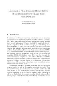
Kenya’s education system comprises eight years of primary school, four years of secondary school, and four years of university. Children must be at least 6 years old before enrolling in the first year of primary. According to the 1999 Kenyan Census, 91% of 15-25 year olds had attended some primary school, but only 68% had completed primary. As can be seen in Figure 1, there was significant geographic variation in primary school attendance prior to 2003. Those in and around the capital city Nairobi had nearly universal primary attendance, while less than half of those in the northeast region of the country had ever attended primary. Between 1991 and 2003, the Gross Enrollment Ratio (GER) in primary school remained relatively constant at 90%. Public schools charged an average of US$16 per year in 1997 although this varied widely, with some schools charging as much as US$350 per year (World Bank, 2004). Kenya eliminated school fees for all public primary schools in the country shortly after the election of a new government in December 2002. Beginning with the new school year in January 2003, the nationwide policy mandated public schools to admit all children seeking admission and prevented schools from charging any fees or levies. Primary enrollment increased 18% (900,000 students) within the first year of FPE (World Bank, 2009), resulting in a GER of around 104%, well above the average of 79% across sub-Saharan Africa (World Bank, 2004). Schools received a capitation grant of US$14 per 5

.756 .621 .521 .227 .125 .063 .046 .04 .038 .02 .015 .013

Figure 1: Share of 15-25 year olds that never attended primary school (1999 Census) Notes: Lightest color are subregions in the bottom decile and darkest color are those in those in the top decile.

6

student, jointly financed by the Kenyan government and external donors. Despite the massive increases in school enrollment resulting from FPE, Lucas and Mbiti (2012a) find that the program had a limited negative impact on the academic performance of students who would otherwise have attended primary. Taken together, we view the program as achieving a significant expansion in access to primary education without considerable changes in quality.

2.2

Financial Inclusion in Kenya

Compared to other countries at the same level of economic development, Kenya has remarkably high levels of financial inclusion. The most recent cross-country statistics available from the 2014 Global Findex surveys indicate that 75% of Kenyan adults aged 15 and over have a formal account, substantially higher than the 43% average for lowermiddle income economies but still below the 91% average for high income economies (Demirguc-Kunt et al., 2015). A large part of Kenya’s financial advantage comes from mobile banking – 58% of adults have a mobile financial account, greatly exceeding the 2% worldwide average. Kenya’s mobile money revolution began when Safaricom (the leading telecommunications company) launched M-PESA as a basic money transfer service in March 2007. This technology later expanded with the launch of M-Shwari in November 2012 as a basic savings and loan product. Users can now earn interest on their savings account and have instant access to short term micro credit loans.4 Access to mobile money generates significant benefits including improving risk sharing by facilitating transfers across social networks and lowering prices of money transfer competitors (Aker and Mbiti, 2010; Jack and Suri, 2014; Mbiti and Weil, 2015). Beneath Kenya’s high levels of formal inclusion, there are still multiple indicators of financial fragility. Although saving rates are higher in Kenya (76%) than in high income economies (67%), the adoption of formal saving is substantially lower (30% versus 47%) and so is the likelihood of saving for old age (18% compared to 37%). Additionally, there are persistent disparities in access to formal financial services. Women, younger adults, and those with lower incomes are substantially less likely to have a formal account. Inequalities exist even with respect to access to mobile money: M-PESA users are more educated, urbanized, wealthier, and more likely to have a bank account than are nonusers (Mbiti and Weil, 2015). 4 See

http://www.safaricom.co.ke/personal/m-pesa and http://www.safaricom.co.ke/personal/mpesa/do-more-with-m-pesa/m-shwari for more details (accessed on March 3, 2017).

7

While the minimum age to open an independent bank account in Kenya is 18, most banks offer joint account options that enable minors to open an account with an adult co-signer. Hence, 34% of 16-18 year olds report ever having a formal financial account.5 Overall, Kenya’s financial landscape is precocious but there is a broad scope for improvement in financial security especially for individuals in marginalized groups.6 The expansion of access to primary schooling therefore provides an ideal opportunity to study the causal effects of education on the financial outcomes of youth.

3

Empirical Methodology

3.1

Reduced-Form Estimates

Although Kenya abolished fees for all public schools in the country simultaneously, the effective impact of FPE varied based on the number of children potentially induced to attend primary school in a given location. Essentially, the program had a higher intensity in places where a lower share of school-age children were attending primary school before the reform. Similarly, older people who were already past the typical schoolgoing age would be less likely to benefit from free primary schooling than younger people in the same location. Age and location of birth therefore both determine the intensity of an individual’s exposure to the FPE program.7 This cohort and location-based variation inspire the following reduced-form specification: Yirc = β 0 + ∑ (d a × Intensityr ) β 1a + X i0 Π + δr + δc + ε irc (1) a

where Yirc is an outcome of interest for individual i in subregion r born in cohort c. Intensityr is the intensity of the FPE program in subregion r (defined as the share of 15-25 year olds born in subregion r that did not attend primary school, based on the 1999 Census).8 d a is an indicator for being age a in 2003. X i is a vector of individual characteristics including gender, religion, and marital status. δr is a fixed effect for each of the 13 subregions and δc is a fixed effect for each birth year. This specification allows us to flexibly estimate the impact of the FPE program separately by age. 5 Authors’

calculations using data from the 2015 FinAccess survey. studies on interventions to increase financial inclusion in Kenya include Dupas and Robinson (2013); Dupas, Keats and Robinson (2015); Schaner (2016). 7 Duflo (2001) uses a similar strategy to estimate the effect of Indonesia’s 1973 school construction program on educational attainment and earnings. 8 We use subregions as our geographic area for this measure because the sample in the financial access survey we analyze is representative at this level. 6 Recent

8

To estimate the full effect of exposure to FPE, our preferred specification restricts our sample to six cohorts of interest. Our treatment cohorts consist of individuals aged 4-6 years old when FPE went into effect in 2003, and thus 16-18 years of age at the time our survey data were collected in 2015. Since children can begin primary school if they are at least 6 at the start of the school year, everyone in these cohorts would have had the opportunity to pursue all eight years of primary school under the FPE program. Our counterfactual age cohorts consist of those who would have been 16-18 in 2003 and thus 28-30 in 2015. Since primary school in Kenya is 8 years long, individuals in these age cohorts would have largely completed primary school by the time the program went into effect. Indeed, only 11% of 16-18 year olds were enrolled in primary school in the 1999 Kenyan census.9 As with our first specification, our preferred estimates exploit geographical variation in treatment intensity based on pre-FPE levels of primary school enrollment. Additionally, we compare two cohorts – the affected cohort that would have been 4-6 years old in 2003 and thus would have had their entire primary education for free; and the unaffected cohort who were 16-18 at the time of the reform and generally too old to take advantage of the FPE program. We use the following difference-in-differences specification to identify the impact of free primary education on our outcomes of interest: Yirc = β 0 + (FPEc × Intensityr ) β 1 + X i0 Π + δr + δc + ε irc

(2)

where FPEc is a dummy variable equal to one if age cohort c was exposed to the reform (aged 4-6 in 2003) and equal to zero if not (aged 16-18 in 2003). δr is a fixed effect for each of the 13 subregions and δc is a fixed effect for each of the six age cohorts. We cluster standard errors at the subregion level. Since having only thirteen clusters may lead to over-rejection of the null hypothesis, we follow Cameron, Gelbach and Miller (2008) and also present wild bootstrap clustered p-values.

3.2

Instrumental Variables Estimates

While the above reduced-form specification provides an estimate of the impact of free primary education on our main outcomes, we are also interested in the causal effects of education per se, not merely the effect of the FPE program. To estimate the causal 9 There

were reports of older students entering primary school due to FPE, but this would only work against our finding significant effects. We do not use 14 and 15 year olds in our counterfactual age cohort since 48% of 14 year olds and 33% of 15 year olds were still enrolled in primary school in the 1999 census. Thus, a substantial portion of youth in these age cohorts would have benefited from FPE.

9

effects of education on our outcomes of interest, we would ideally estimate the following Ordinary Least Squares (OLS) equation: Yirc = α0 + α1 Educationirc + X i0 Λ + δr + δc + eirc

(3)

where Educationirc is the years of education completed by individual i in subregion r born in cohort c. Education is potentially endogenous to our outcome variables however, primarily because individual education levels are unlikely to be random, even conditional on observables and age and subregion fixed effects. We therefore implement a Two-Stage Least Squares (2SLS) estimation strategy using intensity of exposure to the FPE program as an instrument for the years of education completed by those in our sample. In particular, we instrument for education using the following first-stage equation: Educationirc = γ0 + (FPEc × Intensityr ) γ1 + X i0 Γ + δr + δc + uirc

(4)

where FPEc × Intensityr is the excluded instrument. Under the standard assumptions for a valid instrumental variable (IV), this approach yields the average causal effect of a year of education for the subgroup of compliers (individuals induced to complete an additional year of schooling as a result of exposure to free primary education). We discuss the validity of the IV assumptions when we present our results and robustness checks below.

4

Data

Our main source of data is the 2015 Kenya FinAccess household survey conducted from August through October 2015 by the Central Bank of Kenya (CBK), the Kenya National Bureau of Statistics (KNBS) and Financial Sector Deepening Kenya (FSD Kenya). This survey measures access to and demand for financial services for a nationally representative sample of 8,665 individuals aged 16 and above. We include the survey weights in all of our analysis and the sample is representative down to the level of 13 subregional clusters. Table 1 presents summary statistics for our restricted sample of 1,619 individuals aged 16-18 and 28-30. Within this sample, 93% attended at least some primary school, 70% completed primary, and 49% attended at least some secondary school. We do not observe years of education in the data, only education level ranging from none to university degree. To facilitate the interpretation of our results we impute years

10

Table 1: Demographic Summary Statistics Mean

Med.

Education level 3.446 Some primary 0.931 Completed primary 0.701 Some secondary 0.487 Years of education (censored) 7.933 Age 23.682 Female 0.508 Currently married 0.434 Christian 0.897 Muslim 0.083 FPE 0.450 Unemployment rate (1999) 0.196 Intensity 0.103 Intensity (Female) 0.125 Intensity (Male) 0.083

3.0 1.0 1.0 0.0 8.0 28.0 1.0 0.0 1.0 0.0 0.0 0.171 0.038 0.039 0.037

SD

Min.

Max.

Obs.

1.434 1 7 0.254 0 1 0.458 0 1 0.500 0 1 3.561 0 12 6.104 16 30 0.500 0 1 0.496 0 1 0.304 0 1 0.276 0 1 0.498 0 1 0.087 0.109 0.435 0.183 0.013 0.756 0.214 0.012 0.831 0.155 0.014 0.689

1619 1619 1619 1619 1619 1619 1619 1617 1619 1619 1619 1619 1619 1008 611

Notes: Education level takes on a value from 1-7, where 1=None, 2=Some primary, 3=Completed primary, 4=Some secondary, 5=Completed secondary, 6=Technical training after secondary, and 7=University degree. Years of education spans from 0-12, where 0=None, 4=Some primary, 8=Completed primary, 10=Some secondary, 12=Completed secondary, technical training after secondary, or university degree. The sample includes 1,008 females and 611 males. All statistics are calculated using sampling weights, the weighted sample is nationally representative at the subregion level.

11

of education such that none is 0 years, some primary is equivalent to 4 years, completing primary is 8 years, some secondary is 10 years, and completing secondary or more is 12 years. Since our treated, younger cohort is 16-18 years of age, we set the maximum number of years of education to 12 for all of those in our sample.10 By this measure, the average respondent in our sample has 7.9 years of education. We take advantage of the detailed survey questions to construct unique indicators for three dimensions of financial well-being: financial inclusion, financial capability, and economic self-sufficiency. Table 2 summarizes our outcomes. We measure financial inclusion using a series of questions about the use of specific bank products, both currently and at any point in the past. The survey explicitly distinguishes between traditional and mobile banking. When excluding the most common forms of mobile money (M-Shwari and M-PESA), only 29% of the sample had ever banked and 24% currently had a bank product. When including M-Shwari and M-PESA as bank products, 62% had ever used a bank product but only 30% were currently using one. We also separately identify individuals who have a formal saving, loan/credit, or insurance product. Respectively, 29%, 9% and 19% currently had one of these products. To measure financial capability, we start with financial literacy using a set of questions that ask how many of the following nine financial terms respondents have heard of: savings account, interest, shares, collateral, guarantor, investment, inflation, pension, and mortgage. On average, respondents in our sample had heard of 4.6 of these items. Although this measure is a subjective assessment of financial literacy, it generates meaningful variation with responses that span the full range from 0 to 9. To complement this subjective measure, we also use two questions on effective numeracy: (1) “You are in a group and win a promotion or competition for KSh 100,000. With 5 of you in the group, how much do each of you get?" and (2) “You take a loan of KSh 10,000 with an interest rate of 10% a year. How much interest would you have to pay at the end of the year?". Respondents could give an explicit answer or say “I don’t know". We adopt the survey-provided scale and assign respondents a value of high (3), medium (2), or low (1), where high is answering both questions correctly, medium is answering one correctly, and low is answering both either incorrectly or with “I don’t know". The average numeracy is 2.0 in our sample, with 66% of respondents correctly answering the first question and 37% correctly answering the second one. Our two measures of financial literacy differ from the standard Big Three questions used in the literature, which assess conceptual understanding of compound interest, 10 As

a robustness check, we also report estimates that use the completion of a given education level as our measure of schooling.

12

Table 2: Outcome Summary Statistics

Financial Outcomes Ever banked (excl. Mpesa) Ever banked (incl. Mpesa) Currently banked (excl. Mpesa) Currently banked (incl. Mpesa) Ever formal savings (incl. Mpesa) Currently formal savings (incl. Mpesa) Ever formal loan/credit (incl. Mpesa) Currently formal loan/credit (incl. Mpesa) Currently has an insurance product Financial literacy Effective numeracy Forward looking retirement No retirement plans Public/private safety net retirement Member of informal savings group Able to get money in case of emergency Have a safe place to save money Improved financially over year Owns mobile phone Earned any income Monthly income Log (monthly income) Primary Money Sources Farming Employed Casual employment Self-employed Family/friends/spouse Other sources Distance to Nearest Bank branch Mobile money agent Bank agent Don’t Know Distance to Nearest Bank branch Mobile money agent Bank agent

13

Mean

Med.

SD

Min.

Max.

0.290 0.622 0.236 0.300 0.344 0.290 0.170 0.085 0.186 4.646 2.036 0.497 0.203 0.149 0.363 0.337 0.871 2.207 0.662 0.718 9670 8.666

0.0 1.0 0.0 0.0 0.0 0.0 0.0 0.0 0.0 5.0 2.0 0.0 0.0 0.0 0.0 0.0 1.0 2.0 1.0 1.0 3000 8.700

0.454 0.485 0.425 0.458 0.475 0.454 0.376 0.278 0.389 2.735 0.806 0.500 0.402 0.357 0.481 0.473 0.335 0.832 0.473 0.450 23325 1.348

0.194 0.097 0.204 0.153 0.326 0.025

0.0 0.0 0.0 0.0 0.0 0.0

0.396 0.297 0.403 0.360 0.469 0.155

0 0 0 0 0 0

1 1 1 1 1 1

1619 1619 1619 1619 1619 1619

2.494 1.774 2.185

2.0 2.0 2.0

1.183 1.076 1.173

1 1 1

9 9 9

1521 1568 1409

0.046 0.016 0.111

0.0 0.0 0.0

0.210 0.125 0.314

0 0 0

1 1 1

1619 1616 1613

0 1 0 1 0 1 0 1 0 1 0 1 0 1 0 1 0 1 0 9 1 3 0 1 0 1 0 1 0 1 0 1 0 1 1 3 0 1 0 1 0 400000 4.605 12.899

Obs. 1619 1619 1619 1619 1619 1619 1619 1619 1619 1619 1619 1606 1606 1606 1619 1619 1619 1619 1619 1617 1617 1129

inflation, and risk diversification (Lusardi and Mitchell, 2014; Hastings, Madrian and Skimmyhorn, 2013). Nonetheless, our alternative measures have crucial advantages. The effective numeracy questions were open ended rather than multiple choice, allowing us to distinguish between a correct calculation and a lucky guess. Additionally, despite being substantially less complicated than the Big Three questions, our measures yield far from uniformly correct responses and therefore have discriminatory power that a more complex measure may have missed given the low levels of basic numeracy in our setting. Finally, familiarity with financial concepts and effective numeracy are both desirable factors that one could reasonably expect to boost financial capability. Beyond focusing on financial literacy, we examine financial capability more broadly. To measure longer-term well-being, we use a question about retirement planning: “How do you intend to make ends meet in your old age?" We define forward looking individuals as those who intend to draw on savings, a pension, provident fund, retirement savings plan, or income from their investments (50%). We define non-forward looking individuals as those who “have no plans” or “don’t know” (20%). We also identify those who intend to rely on a social safety net namely children, other family members, or a government fund for the old (15%). Despite the relatively young age of respondents in the younger cohort, 50% have a forward-looking retirement plan and this is not statistically different for the older cohort. (Appendix Table A1 reports variable means for each cohort and Appendix Table A2 reports variable means by gender.) We analyze participation in informal saving groups to assess the possibility that participation in the formal financial sector displaces participation in informal groups, 36% of respondents regularly contributed to an informal savings group. The survey also asks about individuals’ ability to get money in case of an emergency and to store money in a safe storage place.11 Finally, we examine a subjective assessment of financial well-being: “Compared to one year ago would you say your financial life has improved, remained the same, or worsened?”. The average response was 2.2 on a welfare-increasing scale from 1 to 3. To understand the mechanisms linking education and financial outcomes, we examine economic self-sufficiency drawing on survey questions about employment and income. Respondents were asked what their main source of money was, with 20% citing casual employment, 19% farming, 15% self-employment, 10% formal employment, and 2.5% income from other sources. 32% of the sample relied on friends, family, or their 11 Specifically,

the survey asked: “If you needed KSh 2,500 (for rural respondents) or KSh 6,000 (urban) within three days in case of an emergency would you be able to get it?” and “If you received KSh 500 (rural) or KSh 5,000 (urban) do you have a safe place you can save this money?”. A third of respondents could get money in an emergency and 87% had a safe place to save money.

14

spouse as their primary source of money. A total of 72% reported earning some income on their own, with an average reported monthly income of KSh 9,670 (US$92), including zeros. We summarize these multiple outcomes using a set of indices based on Kling, Liebman and Katz (2007). Essentially, we subtract the mean and divide by the standard deviation of the “control” group for each outcome (individuals aged 28-30 in the Central subregion, which had the highest pre-FPE enrollment rate of 99%). We then take an equally weighted mean of the resulting z-scores.12 Our second data source is the Integrated Public Use Microdata Series, International 5% sample of the 1999 Kenyan census conducted by KNBS (Minnesota Population Center, 2015). As outlined in the preceding section, our identification strategy exploits geographical variation in treatment intensity (Intensityr ), based on pre-FPE educational attainment. By subregion of birth, we calculate the proportion of 15 to 25 year olds who had never attended primary school. The pre-FPE proportion of youth that had never attended primary is an intuitive measure of intensity because it focuses on the marginal compliers. Figure 1 illustrates the geographic variation in Intensityr . The average individual in our sample lived in a subregion where 10% of 15 to 25 year olds in 1999 had never attended primary school. This ranged from 1.3% in the Central subregion to 75% in the Northeastern subregion. As a robustness check, we calculate gender-specific treatment intensities. The average female in our sample resides in a subregion where 12% of females aged 15-25 in 1999 had never attended primary school, the comparable statistic is 8% for males.13 We also use the 1999 census to calculate unemployment rates by subregion as a proxy for existing economic conditions before the FPE reform. Combining individual-level data from the 2015 survey with our subregion-level FPE treatment intensity measure from the 1999 census allows us to adopt a difference-indifferences estimation strategy under the key identifying assumption that differentially 12 Although

we separately report estimates for the full set of available outcomes, our summary indices focus on outcomes occurring for at least 5% of the younger cohort to account for the fact that we may not be able to observe differences in low-probability outcomes at young ages, biasing us towards a mechanical result of significant difference-in-differences estimates even when there are no real effects. Specifically, our financial inclusion index comprises indicators for ever having banked, currently being banked, and ever having a formal savings account, all including mobile banking; our financial capability index comprises financial literacy, effective numeracy, forward looking retirement, being a member of an informal savings group, being able to access funds in an emergency, having a safe place to store money, and whether a respondent’s financial life has improved in the last year; and our economic self-sufficiency index comprises an indicator for earning any income, income earned, and an indicator for relying on another source (usually employment) besides family, friends or a spouse as a primary source of income. 13 Appendix Table A3 documents the intensity measures for each subregion.

15

affected subregions had parallel trends in financial outcomes prior to the program’s implementation (i.e., the differences between high and low intensity areas would have remained unchanged in the the absence of the FPE program). This assumption is not testable but we use data for 40-42 year olds (28-30 in 2003) to conduct a falsification exercise with a placebo reform for older cohorts not exposed to FPE, to provide supportive evidence.

5

Results

We begin by documenting that FPE increased education levels. We then analyze effects on financial inclusion and financial capability. We turn to effects on economic selfsufficiency before analyzing mechanisms. Finally, we present two stage least squares estimates of the effect of education on financial outcomes, with FPE intensity as an instrument for education.

5.1

Impact of FPE on Educational Attainment

Figure 2 presents a visual illustration of the effect of FPE on educational attainment. We plot coefficients and 95% confidence intervals for the vector of (d a × Intensityr ) interaction terms in our flexible specification that allows the impact of the program to vary by age (equation 1). The largest impacts of the program on years of education appear to be for those in the youngest cohorts. Consistent with the parallel trends assumption, we find insignificant differences in education levels for older adults who would have been above the typical primary school age by the time FPE began in 2003. Table 3 presents results from estimating the impact of free primary education on the years of education completed. Column 1 includes only the FPEc indicator, Intensityr , and the (FPEc × Intensityr ) interaction. Column 2 includes cohort fixed effects and an indicator for females.14 Column 3 additionally includes subregion fixed effects, reflecting to our specification outlined in equation 2.15 Overall, the results indicate that greater exposure to the FPE program increased the highest education level achieved, where moving from the lowest to highest intensity subregion increased education by about 3.2 years.16 Appendix Table A4 presents results from estimating the impact of free primary education on the highest education level 14 We

exclude FPEc as it is collinear with the cohort fixed effects. exclude Intensityr as it is collinear with the subregion fixed effects. 16 These effect sizes are based on the difference in intensity for the highest and lowest subregion displayed in Appendix Table A3. For the pooled sample, this was 0.756 − 0.013 = 0.743 15 We

16

10 5 0 -5 -10

4

6

8

10

12

14 16 18 Age in 2003

20

22

24

26

28

Figure 2: Coefficients on Interactions of Age and FPE Intensity for Years of Education Notes: Dependent variable is imputed years of education censored at 12 years, where 0=None, 4=Some primary, 8=Completed primary, 10=Some secondary, 12=Completed secondary. Plots coefficients on an interaction of cohort and intensity, with the age 28 in 2003 cohort as the excluded group. 95% confidence intervals presented based on standard errors clustered at the subregion level.

Table 3: Years of Education (Censored at 12) (1) Mean Dep. Var. [SD] FPE × Intensity

FPE

Intensity

Observations Adjusted R2 FPE×Intensity F-stat Cohort FE Subregion FE

(2) 7.933 [3.561]

4.514*** (1.199) [0.004] -0.260 (0.431) [0.595] -9.757*** (1.134) [0.002] 1619 0.182 14.17

4.697*** (1.059) [0.000]

-9.729*** (1.048) [0.002] 1619 0.191 19.68 X

(3) 4.351*** (1.134) [0.004]

1619 0.225 14.72 X X

Note: Robust standard errors in parentheses clustered by 13 subregions. ∗ p < 0.10, ∗∗ p < 0.05, ∗ ∗ ∗ p < 0.01. Wild bootstrap clustered p-values in brackets with 999 replications. Dependent variable is imputed years of education censored at 12 years, where 0=None, 4=Some primary, 8=Completed primary, 10=Some secondary, 12=Completed secondary.

17

achieved. The results are similar to those using years of education as an outcome and show that the largest effects of FPE were on the likelihood of completing some primary. These reduced-form results establish a strong first stage – free primary education increased the education levels of those exposed, and this impact was larger in subregions that had lower primary attendance prior to the program’s implementation.

5.2

Impact of FPE on Financial Outcomes

Table 4 presents the reduced-form impacts of free primary education on financial inclusion, financial capability, and economic self-sufficiency (illustrated in Figure 3) We estimate an identical set of specifications to those in Table 3 but with a given outcome of interest instead of education as the dependent variable. Our preferred specification indicates that moving from a pre-FPE primary nonenrollment rate of 0 to 100% increases financial inclusion by 0.76 standard deviations of the control group mean (column 3), increases financial capability by 0.31 standard deviations (column 6), and increases economic self-sufficiency by 1.1 standard deviations (column 9). Scaling these effects based on the variation observed in our sample implies that going from the highest to the lowest intensity subregion in our sample increased financial inclusion, financial capability, and economic self-sufficiency by 0.57, 0.23, and 0.82 standard deviations respectively. All of these estimates are statistically significant using the clustered standard errors, however, the effects on financial inclusion are no longer significant when we use the more conservative wild bootstrapped standard errors. Decomposing the financial inclusion index, reduced-form estimates for specific outcomes in Table 5 indicate that those in the highest intensity subregions were 26 percentage points more likely to have ever banked than those in the lowest intensity subregions when including the use of mobile banking, relative to a mean of 62%. This estimate is statistically significant using both sets of standard errors. We find similar effects on the likelihood of ever having a formal saving account, but smaller and marginally significant effects on the likelihood of currently having any formal account. We further investigate the effects of FPE on financial inclusion using data on specific bank products used in Appendix Table A5. We find significant increases in the likelihood of currently and ever having a formal savings product and in ever using a formal loan or credit product. The coefficient for insurance products indicates an increase in their use but is not statistically significant. Consistently, the strongest effects on banking access, in terms of both magnitude and statistical significance, are found only when we include mobile banking.

18

1

0

4

6

8

12

14 16 18 Age in 2003

20

22

4

24

6

26

8

28

12

14 16 18 Age in 2003

20

(a) Financial inclusion

10

22

4

24

6

26

8

10

12

14 16 18 Age in 2003

20

22

(c) Economic self-sufficiency

28

Figure 3: Coefficients on Interactions of Age and Intensity for Summary Indices

(b) Financial capability

10

2 1 0 -1

24

26

28

Notes: Dependent variable is a) financial inclusion summary index (comprised of ever having banked, currently being banked, and ever having a formal savings account, all including mobile banking), b) financial capability summary index (comprised of financial literacy, effective numeracy, forward looking retirement, being a member of an informal savings group, able to access funds in an emergency, have a safe place to store money, and whether respondent’s financial life has improved in the last year), and c) economic self-sufficiency summary index (comprised of an indicator for earning any income, income earned, and an indicator for relying on another source besides family, friends or a spouse as a primary source of income). Plots coefficients on an interaction of cohort and intensity, with the age 28 cohort as the excluded group. 95% confidence intervals presented based on standard errors clustered at the subregion level.

-1

2 1 0 -1 -2

19

20

(1) 0.889** (0.330) [0.470] -1.198*** (0.026) [0.002] -1.403*** (0.356) [0.054] 1619 0.333 -1.387*** (0.314) [0.048] 1619 0.363 X

(2) 0.968*** (0.259) [0.193]

1619 0.420 X X

(3) 0.764** (0.275) [0.312]

Financial Inclusion (4) (5) (6) 0.350** 0.390*** 0.308** (0.115) (0.109) (0.117) [0.000] [0.000] [0.000] -0.318*** (0.043) [0.002] -0.949*** -0.950*** (0.165) (0.150) [0.002] [0.002] 1619 1619 1619 0.132 0.155 0.196 X X X

Financial Capability

(7) (8) (9) 0.893*** 1.066*** 1.099*** (0.279) (0.220) (0.240) [0.020] [0.000] [0.000] -1.277*** (0.100) [0.002] -0.538*** -0.559*** (0.143) (0.113) [0.002] [0.002] 1619 1619 1619 0.290 0.338 0.350 X X X

Economic Self-Sufficiency

Note: Robust standard errors in parentheses clustered by 13 subregions. ∗ p < 0.10, ∗∗ p < 0.05, ∗ ∗ ∗ p < 0.01. Wild bootstrap clustered p-values in brackets with 999 replications. Dependent variable is a summary index using Kling, Liebman and Katz (2007) method. Columns 2, 3, 5, 6, 8 and 9 additionally control for gender.

Observations Adjusted R2 Cohort FE Subregion FE

Intensity

FPE

FPE × Intensity

Dependent Variable

Table 4: Reduced-Form Results for Summary Indices

Table 5: Reduced-Form Results for Specific Outcomes Panel A: Financial Inclusion Dependent Variable Ever Banked (1) FPE × Intensity

Observations Adjusted R2

Currently Banked (2)

Ever Formal Savings (3)

0.249* (0.138) [0.190] 1619 0.255

0.310** (0.131) [0.060] 1619 0.271

Financial Literacy (1)

Numeracy (2)

Forward Looking Retirement (3)

2.063*** (0.606) [0.000] 1619 0.218

0.210 (0.171) [0.298] 1619 0.073

-0.121 (0.114) [0.336] 1606 0.072

IHST Monthly Income (2)

Not Reliant on Friends/Family/Spouse (3)

4.870*** (0.986) [0.000] 1617 0.383

0.362*** (0.088) [0.004] 1619 0.311

0.354** (0.144) [0.086] 1619 0.400

Panel B: Financial Capability Dependent Variable FPE × Intensity

Observations Adjusted R2

Panel C: Economic Self-Sufficiency Earned Dependent Variable Any Income (1) FPE × Intensity

Observations Adjusted R2

0.403*** (0.096) [0.006] 1617 0.299

Note: Robust standard errors in parentheses clustered by 13 subregions. ∗ p < 0.10, ∗∗ p < 0.05, ∗ ∗ ∗ p < 0.01. Wild bootstrap clustered p-values in brackets with 999 replications. All specifications include subregion and cohort fixed effects and controls for gender. Each cell presents the coefficient on FPE×Intensity from reduced-form estimations of equation 2.

21

In contrast to these effects on financial inclusion, we find limited impacts on broader indicators of financial well-being. Individuals in the highest intensity subregions were familiar with 1.5 more financial terms than those in the lowest intensity subregions (panel B in Table 5). Yet there is no statistically significant impact on effective numeracy, although the coefficient is positive, and there are no significant changes in retirement planning. As Appendix Table A6 illustrates, individuals exposed to FPE are more likely to participate in an informal savings group and are more likely to report being able to get money in case of an emergency. They are no more likely to say they have a safe place to save money or that their financial life has improved over the past year. Since financial inclusion potentially increases risk, we look at responses to shocks as a final outcome. Appendix Tables A7 and A8 report summary statistics on respondents’ experiences of financial shocks in the preceding two years, 79% of respondents experienced some type of shock. Appendix Table A9 indicates that individuals exposed to FPE were more likely to use savings to deal with a financial shock to their household rather than relying on help from others or doing nothing. Altogether, these results suggest that education increases the use of both formal and informal financial services and facilitates access to money in an emergency but does not appear to improve effective numeracy, long-term financial planning, or subjective assessments of financial well-being.

5.3

Impact of FPE on Economic Self-Sufficiency

In addition to evaluating financial outcomes, we explore the returns to education in terms of income and employment in panel C of Table 5. Column 1 reports income effects on the extensive margin. Moving from the lowest to highest intensity subregion resulted in a 30 percentage point increase in the likelihood of earning any income. To examine impacts on the intensive margin, we begin by using the inverse hyperbolic sine transformation of monthly income (Burbidge, Magee and Robb, 1988) and the log of (1 + monthly income), retaining the full sample including those who did not earn any income. We find very large increases in income, with a coefficient of 4.87 for the inverse sine transformation of earnings (3.62 going from the lowest to the highest intensity subregion).17 Appendix Table A10 investigates the log of monthly income as the dependent vari17 By comparison, Duflo, Dupas and Kremer (2017) find that winning a secondary school scholarship in Ghana increased the inverse hyperbolic sine of earnings at age 25 by 0.308. They also find a much smaller (10%) increase in the likelihood of earning any income, compared to our 30 percentage point increase on a mean of 47% for the younger cohort.

22

able. Note that this drops all of the zeros from our sample. In column 1, we see that the magnitude of the impact on income earners is still very large, moving from the lowest to the highest intensity subregion increased log monthly income by 1.27. Appendix Table A11 investigates the impact of FPE on respondents’ primary source of money. The survey asked the primary source of money in the last 12 months out of farming, employment, casual work, self-employment, family/friends/spouse, or other sources.18 Reduced-form results in column 1 indicate that moving from the lowest to highest intensity subregion is associated with being 27 percentage points less likely to rely on family, friends, or a spouse as a primary source of money, compared with a sample mean of 32%. Additionally, respondents were 23 percentage points more likely to rely on self-employment and 11 percentage points more likely to rely on employment. These estimates are large in magnitude compared to a sample means of 15% and 10%, respectively. Altogether, we find large impacts on income and employment outcomes.

5.4

Heterogeneity by Gender

Having estimated the overall effects of FPE, we now turn to consider gender-specific effects. Appendix Table A3 indicates not only significant heterogeneity in baseline levels of our intensity measure, primary attendance from the 1999 census, across subregions but also by gender within subregions. For example, in the Coastal subregion 12.9% of males 15-25 had never attended primary school, while this was 31.3% for females. Hence, it is possible this heterogeneity in baseline primary attendance levels by gender could generate heterogeneity in the impact of FPE by gender. In order to test for this possibility, we repeat our reduced-form analysis but introduce an additional interaction between FPE, intensity, and female to our baseline specification. Appendix Table A12 presents these results, where panel A uses the average intensity from column 1 in Appendix Table A3 and panel B uses gender-specific intensities from columns 2 and 3. There is some evidence of a larger impact for females on financial inclusion, but not for years of education, financial capability, or economic self-sufficiency.

5.5

Analysis of Mechanisms

Thus far, we have presented evidence that free primary education increased financial inclusion and had moderate impacts on financial capability. However, it also led to higher income and lower reliance on family, friends, and spouses for money. It therefore 18 Other

sources included subletting of property, renting equipment, investments, assistance from NGOs or the government.

23

Table 6: Including Demographic and Income Controls Additional Control Dependent Variable Financial Inclusion

Religion & Income Money Distance to Bank Products Base (1)

0.764** (0.275) [0.302] Financial Capability 0.308** (0.117) [0.000] Econ. Self-Sufficiency 1.099*** (0.240) [0.000] Observations 1619

Marriage (2)

Cubic (3)

Source (4)

Branch (5)

0.791** (0.283) [0.276] 0.354** (0.118) [0.004] 1.080*** (0.241) [0.000] 1619

0.449 (0.300) [0.457] 0.100 (0.133) [0.466] 0.539*** (0.156) [0.010] 1617

0.557** (0.247) [0.303] 0.218* (0.114) [0.062] 0.321*** (0.086) [0.000] 1619

0.740*** (0.200) [0.008] 0.156 (0.094) [0.174] 1.035*** (0.264) [0.000] 1619

Agent (6)

Mpesa (7)

0.684*** 0.809*** (0.177) (0.150) [0.000] [0.000] 0.123 0.202** (0.081) (0.083) [0.184] [0.016] 1.049*** 1.002*** (0.262) (0.272) [0.002] [0.002] 1613 1616

Note: Robust standard errors in parentheses clustered by 13 subregions. ∗ p < 0.10, ∗∗ p < 0.05, ∗ ∗ ∗ p < 0.01. Wild bootstrap clustered p-values in brackets with 999 replications. All specifications include subregion and cohort fixed effects and column 1 controls for gender. Dependent variable is a summary index using Kling, Liebman and Katz (2007) method.

seems plausible that the link between higher financial inclusion, financial capability, and education primarily operates through increased income and changes in employment outcomes. We examine this possibility and other potential causal mechanisms below. Table 6 displays our main results with controls for different factors that could be channels through which increased financial inclusion, financial capability, or economic self-sufficiency could be occurring. Column 1 repeats our baseline results from columns 3, 6 and 9 of Table 4 for comparison. Column 2 additionally controls for marital status and religion, and finds that this does not change our results.19 Column 3 controls for a cubic polynomial of monthly income. This attenuates financial inclusion by nearly half, and financial capability by about two-thirds such that both point estimates are no longer statistically different from zero. Column 4 controls for whether the primary source of money was farming, employment, self-employment, casual employment, family/friends/spouse, or other sources. This also attenuates the magnitude of the coefficients on financial capability and inclusion, but not by as much as when we control for income. We also examine the potential role of supply-side changes. Results in Appendix Table A14 show that those exposed to FPE reported being closer to banking products. There19 Consistent

with this finding, reduced-form results presented in Appendix Table A13 indicate that FPE did not significantly impact religion or the probability of being married.

24

fore, it is possible that the intensity of FPE was simply correlated with an expansion of financial services. Columns 5-7 report results controlling for the distance reported to the nearest bank branch, bank agent, and M-PESA agent. Controlling for these factors does not meaningfully change the magnitude of our estimated effects on financial inclusion, but appreciably increases the precision of our estimates. Thus, changes in financial inclusion do not appear to result from changes in access to financial services. In contrast, this same exercise attenuates the estimated effects on financial capability by 34%-60%, suggesting that proximity to financial products could partly explain improvements in our proxies for financial decision-making. Controlling for marital status, religion, and distance to banking products does not meaningfully change the results for economic self-sufficiency. Overall, these results provide evidence that employment outcomes are likely to be an important channel through which free primary education increased financial inclusion and capability.

5.6

Instrumental Variables Estimates

We have presented evidence that free primary education in Kenya led to higher levels of financial inclusion, financial capability, and economic self-sufficiency. Nonetheless, these results do not allow us to make inferences about the causal impact of educational attainment on our main outcomes of interest. In order to directly quantify the effects of education, we impose some additional assumptions and present results from a two-stage least squares estimation. Beyond the necessary criteria for our difference-in-differences strategy, the IV approach requires relevance of the instrument, monotonicity, and satisfaction of an exclusion restriction. Our original results on the impact of FPE on years of education in Table 3 represent the first-stage in our two-stage estimation. In our preferred specification in column 3, the F-stat for the excluded instrument (FPE × Intensity) is 14.7. This establishes that the instrument is relevant and sufficiently strong. To satisfy the monotonicity condition, we need that no one would defy the encouragement of free primary education. Essentially, there should be no individuals who would attend primary if it was not free but refuse to attend once it is free. Based on the available evidence, this condition is likely to be satisfied. Although many students reportedly shifted from the public to private sector, we are not aware of any reports of students withdrawing from school altogether, consistent with the trend of an aggregate increase in school enrollment following the introduction of FPE. Under our framework, the final IV assumption implies that the intensity of free primary education must be correlated with our outcomes of

25

Table 7: OLS and 2SLS Results OLS (1)

Dependent Variable Financial Inclusion

Financial Capability

Economic Self-Sufficiency

Observations 1st Stage F-Stat

2SLS (2)

0.095*** 0.175*** (0.008) (0.052) [0.000] 0.067*** 0.071*** (0.005) (0.021) [0.000] -0.002 0.253*** (0.007) (0.066) [0.790] 1619

1619 14.84

Note: Robust standard errors in parentheses clustered by 13 subregions. ∗ p < 0.10, ∗∗ p < 0.05, ∗ ∗ ∗ p < 0.01. Wild bootstrap clustered p-values in brackets with 999 replications. All specifications include subregion and cohort fixed effects and controls for gender. Each column presents the coefficient on years of education, censored at 12 years, from estimates of equation 3. Column 1 presents simple OLS results while column 2 presents two-stage least squares estimates with FPE×Intensity as the excluded instrument. Dependent variable is a summary index using Kling, Liebman and Katz (2007) method.

interest only through the level of education attained by those in our sample. The most obvious violation for this assumption would be if FPE affected the quality as well as the level of education received. As discussed earlier, Lucas and Mbiti (2012a) find limited changes in educational quality after the introduction of FPE. Under these assumptions, we can estimate the local average treatment effect (LATE) of education on the financial outcomes of compliers. In our setting, compliers would be those induced by the FPE program to increase their educational attainment. Appendix Table A4 provides evidence that compliers were largely on the margin of obtaining any formal education since completing some primary school is the level with the strongest effect, although there also appears to be a smaller but statistically significant impact on completing secondary. Table 7 presents our first set of results estimating the naive OLS equation 3 in column 1 and then the second stage of a two-stage least squares (2SLS) in column 2. In each case, we report the coefficient on years of education, censored at 12 years. Our 2SLS estimates of the effects of education on financial inclusion are larger than the OLS estimates, with coefficients of 0.175 and 0.095 respectively. The financial capability estimates are comparable (0.067 for OLS and 0.071 for 2SLS). The 2SLS estimates of effects on economic 26

self-sufficiency of 0.253 are considerably larger than the OLS estimates, which are close to zero and statistically insignificant. Appendix Tables A5 and A6 report results for the use of specific banking products and indicators of financial capability with the OLS results in column 2 and 2SLS results in column 3. Higher education levels are correlated with increased access to banking services, higher financial literacy, and higher effective numeracy. 2SLS results in column 3 indicate that each additional year of education is causally linked with being 8.1 percentage points more likely to have ever banked, 5.7 percentage points more likely to be currently banked, being familiar with 0.47 more financial terms, and scoring higher on effective numeracy by 0.05 levels. With the exception of effective numeracy, these are all larger in magnitude then the associated OLS coefficients. A plausible explanation for this is that the marginal compliers in our sample were those induced to attend at least some primary school as opposed to never having any formal education. This population was also likely the poorest in any subregion, so large effects for this population of compliers is not surprising. Columns 2 and 3 of Appendix Table A10 present analogous results but for income. OLS estimates indicate that the raw correlation between years of education and earning any income is zero or slightly negative, however the 2SLS estimates indicate a 9.3 percentage point increase in the likelihood of earning any income for each additional year of education. The OLS estimates for effects on income earned show a statistically insignificant increase, but 2SLS results show a large increase in income per year of education. Appendix Table A11 reports effects on employment outcomes. From OLS estimates in column 2, higher education is associated with a lower probability of casual employment, and a higher probability of employment and relying on family, friends, or a spouse. This estimate could be biased if, for example, those with higher education come from richer families, and those from richer families are more reliant on their family as their primary source of income, particularly when they are younger. 2SLS estimates in column 3 are in line with our reduced-form results. Recall again that our complier population are those from more disadvantaged backgrounds who were induced by FPE to attend primary school when they otherwise would have had no formal education. Based on our IV estimates, an additional year of education generates a 3 percentage point increase in being employed, a 7 percentage point increase in being self-employed, and an 8 percentage point decrease in relying on family, friends, and/or spouse as the primary source of money.

27

6

Robustness Checks

The validity of our preceding analysis depends on several crucial assumptions and we address the main confounding factors in the discussion below. Each row of Table 8 reports an alternative set of estimates from a different robustness check. The dependent variable for each estimate in column 1 is the financial inclusion index, the financial capability index in column 2, and the economic self-sufficiency index in column 3. For comparison, the first row repeats the baseline results from our preferred specification in columns 3, 6 and 9 of Table 4. One potential concern is that other contemporaneous government programs could have targeted subregions with lower economic performance, which also had low primary school attendance levels. We proxy for this possibility by controlling for the pre-FPE unemployment rate in each subregion from the 1999 census, interacted with each age cohort. Our results are robust to these inclusions and our estimates do not significantly change. We also check the robustness of our treatment intensity measure. In our main results we use a subregion-level intensity measure based on average pre-FPE enrollment rates. However, Appendix Table A3 indicates there was variation in intensity for males and females within each subregion. We present alternative estimates using the respective gender-specific intensities for males and females in the sample. These results are in line with our baseline results. An argument could be made that FPE potentially impacted the likelihood of completing primary education, not merely the likelihood of attending primary. We check whether our results change if we redefine intensity as the pre-FPE share of those in each subregion aged 15-25 that never completed primary school, instead of the share that never attended primary school. The results using completed primary as the intensity are of similar magnitude to our baseline results but are less precisely estimated. One limitation of our data is that we only observe where individuals in our sample were residing at the time they were surveyed, not where they were born. In the 1999 Census, 87.3% of 16-18 year olds and 73.5% of 28-30 year olds still lived in their subregion of birth. To address the potential for endogenous migration, we exclude Nairobi and Mombasa since these are the two largest cities in Kenya and attract a large number of migrants from the rest of the country.20 Alternatively, we exclude the 8% of respondents 20 20%

of residents in Nairobi and Mombasa had moved in the last 12 months compared to 6% in the rest of the sample. The two subregions account for 15% of the sample. Moreover, from the 1999 Census, these were the subregions that had the lowest share of residents that were also born there. For example, only 36% of those aged 16-18 and 13% aged 28-30 residing in Nairobi were born there, and this was 50%

28

Table 8: Robustness Checks Dependent Variable - Index Robustness Check Baseline ( N = 1619)

1999 Subregion unemployment ( N = 1619)

Alternative intensities ( N = 1619)

Completed primary intensity ( N = 1619)

Exclude Nairobi and Mombasa ( N = 1446)

Exclude migrants ( N = 1495)

Mobile phone ownership ( N = 1619)

Internet usage ( N = 1619)

Donald-Lang two step estimation ( N = 26)

Placebo for 28-30 vs. 40-42 ( N = 1486)

Financial Inclusion (1)

Financial Capability (2)

Econ. SelfSufficiency (3)

0.764** (0.275) [0.312] 0.735** (0.253) [0.216] 0.805*** (0.232) [0.164] 0.627* (0.324) [0.180] 0.811** (0.277) [0.276] 0.811*** (0.242) [0.137] 0.775** (0.257) [0.130] 0.828*** (0.263) [0.143] 0.837** (0.340)

0.308** (0.117) [0.000] 0.310** (0.119) [0.000] 0.349*** (0.107) [0.000] 0.223 (0.144) [0.162] 0.323** (0.129) [0.000] 0.292** (0.134) [0.048] 0.313*** (0.100) [0.000] 0.346** (0.119) [0.000] 0.422** (0.192)

1.099*** (0.240) [0.000] 1.148*** (0.242) [0.011] 1.051*** (0.216) [0.000] 1.441*** (0.320) [0.016] 0.929*** (0.193) [0.000] 1.125*** (0.229) [0.000] 1.101*** (0.243) [0.000] 1.098*** (0.238) [0.000] 0.907*** (0.241)

0.314* (0.161) [0.124]

-0.014 (0.124) [0.891]

-0.334 (0.201) [0.255]

Note: Robust standard errors in parentheses clustered by 13 subregions. ∗ p < 0.10, ∗∗ p < 0.05, ∗ ∗ ∗ p < 0.01. All specifications include subregion and cohort fixed effects and controls for gender. Wild bootstrap clustered p-values in brackets with 999 replications. Each cell reports the coefficient on FPE × Intensity for a separate regression. Each row focuses on a different robustness check.

29

who moved in the last 12 months. The results from both of these robustness checks are in line with our main results. Given that we find FPE increased mobile banking substantially more than traditional banking, access to mobile telecommunications networks may be driving our results. To explore this possibility, we control for mobile phone ownership and internet usage. Again, this does little to change our results. An alternative to the wild bootstrap cluster that is robust to the possibility of overrejection of the null in the presence of few clusters is the two step method devised by Donald and Lang (2007). We also present results from using this method and they are in line with the main results presented in Table 4.21 Notably, the effects on all three indices are statistically significant. Finally, we construct a placebo FPE treatment using an older cohort. Effectively, we let those aged 28-30 in our sample (16-18 in 2003) be “treated” by FPE and compare them with a control older cohort aged 40-42 in our sample (28-30 in 2003). This check shows a marginally significant positive coefficient for financial inclusion in column 1, however the magnitude of the coefficient is only two-fifths the size and the wild-bootstrap clustered p-value is 0.124. The impact on the other two indices is indistinguishable from zero. Overall, the results from our placebo experiment provide supportive evidence that we are not simply picking up any prior differential trends in our main outcomes of interest.

7

Conclusions

This paper provides new evidence on the causal effects of education on the financial outcomes of young adults using a wide-reaching policy in a developing economy. Our results demonstrate positive impacts on financial literacy, savings, and the use of formal financial services. At the same time, we find smaller improvements in financial capability and significant impacts in economic self-sufficiency, which point to increased earnings as a key causal mechanism. Is FPE a cost-effective strategy to increase financial inclusion? The Kenyan government provided schools a capitation grant of $14 (Ksh 1,020) per student per year (World Bank, 2009). Our 2SLS estimates reported in Appendix Table A5 indicate that completing one additional year of education generates an 8.1 percentage point increase in the likeliand 23% for Mombasa. For all other subregions this ranged from 79% to 99% for 16-18 year olds and 61%-98% for 28-30 year olds. 21 The sample size is only 26 as this method collapses the individual data down to the means within each subregion for the FPE and non-FPE cohorts. The coefficients differ from our baseline estimates because this approach weights each subregion equally.

30

hood of ever having a formal account. A back of the envelope calculation therefore puts the cost of opening one additional bank account at $14/0.081 = $173. Alternatively, the cost of inducing one additional person to currently have a formal account is $14/0.057 = $246. Three common alternative interventions to promote banking are financial literacy training, bank account subsidies, and behavioral approaches such as commitments, reminders, labels, and peer pressure (Dupas et al., 2016, summarize results from 16 recent studies). Most studies do not provide enough information to construct a costeffectiveness estimate. In a notable exception, Dupas and Robinson (2013) evaluate a randomized intervention for rural market vendors and bicycle taxi drivers in Kenya and find that offering a $7.83 subsidy to open a formal bank account generates a 41 percentage point increase in the likelihood of being an active account user (making two deposits within the first six months), implying a cost of $19 per active account. Focusing on a more general population but in a different context, Cole, Sampson and Zia (2011) present estimates from a randomized evaluation for a sample of unbanked households in Indonesia. They estimate that offering subsidies costs $145 per savings account opened and financial literacy training costs $340. By comparison, FPE falls between these two alternatives. This suggests that FPE is a competitive policy tool even under a conservative valuation that isolates the benefit of FPE on the financial inclusion margin, independently of all the other returns to education. We conclude with two caveats. First, our estimates identify the effects of education for a sample of youth (primarily 16-18 year olds). Given the recentness of Kenya’s adoption of FPE in 2003, we cannot yet observe longer run outcomes for the main beneficiaries. Perhaps improvements in financial capability accrue over time. We hope to explore this possibility in future work. Second, we focus on Kenya, where rates of financial inclusion are high relative to other countries at similar levels of economic development, largely due to the prevalence of mobile banking. The effects of education could be rather different in a more traditional banking environment. Indeed, only 6.2% of 16 to 18 year olds in our sample had ever banked in a traditional bank while 33.8% had ever banked once we include mobile banking. Ultimately, our results suggest that digital financial services could be a crucial complement to education in efforts to improve the financial outcomes of youth.

31

References Agarwal, Sumit, John Driscoll, Xavier Gabaix, and David Laibson. 2009. “The Age of Reason: Financial Decisions over the Life-Cycle and Implications for Regulation.” Brookings Papers on Economic Activity, 2009(2): 51–117. Aker, Jenny C., and Isaac M. Mbiti. 2010. “Mobile Phones and Economic Development in Africa.” Journal of Economic Perspectives, 24(3): 207–32. Ashraf, Nava, Dean Karlan, and Wesley Yin. 2010. “Female Empowerment: Impact of a Commitment Savings Product in the Philippines.” World Development, 38(3): 333–344. Bernheim, B.Douglas, Daniel M. Garrett, and Dean M. Maki. 2001. “Education and Saving: The Long-Term Effects of High School Financial Curriculum Mandates.” Journal of Public Economics, 80(3): 435 – 465. Berry, James, Dean Karlan, and Menno Pradhan. 2015. “The Impact of Financial Education for Youth in Ghana.” National Bureau of Economic Research Working Paper 21068. Brown, Meta, John Grigsby, Wilbert van der Klaauw, Jaya Wen, and Basit Zafar. 2016. “Financial Education and the Debt Behavior of the Young.” The Review of Financial Studies, 29(9): 2490. Bruhn, Miriam, Gabriel Lara Ibarra, and David McKenzie. 2014. “The Minimal Impact of a Large-Scale Financial Education Program in Mexico City.” Journal of Development Economics, 108: 184–189. Bruhn, Miriam, Luciana de Souza Leao, Arianna Legovini, Rogelio Marchetti, and Bilal Zia. 2016. “The Impact of High School Financial Education: Evidence from a LargeScale Evaluation in Brazil.” American Economic Journal: Applied Economics, 8(4): 256–95. Burbidge, John B., Lonnie Magee, and A. Leslie Robb. 1988. “Alternative Transformations to Handle Extreme Values of the Dependent Variable.” Journal of the American Statistical Association, 83(401): 123–127. Burgess, Robin, and Rohini Pande. 2005. “Do Rural Banks Matter? Evidence from the Indian Social Banking Experiment.” American Economic Review, 95(3): 780–795. Cameron, A. Colin, Jonah B. Gelbach, and Douglas L. Miller. 2008. “Bootstrap-Based Improvements for Inference with Clustered Errors.” Review of Economics and Statistics, 90(3): 414–427. 32

Cole, Shawn, Anna Paulson, and Gauri Kartini Shastry. 2014. “Smart Money? The Effect of Education on Financial Outcomes.” Review of Financial Studies, 27(7): 2022– 2051. Cole, Shawn, Anna Paulson, and Gauri Kartini Shastry. 2016. “High School Curriculum and Financial Outcomes: The Impact of Mandated Personal Finance and Mathematics Courses.” Journal of Human Resources, 51(3): 656–698. Cole, Shawn, Thomas Sampson, and Bilal Zia. 2011. “Prices or Knowledge? What Drives Demand for Financial Services in Emerging Markets?” Journal of Finance, 66(6): 1933–1967. Demirguc-Kunt, Asli, Leora Klapper, Dorothe Singer, and Peter Van Oudheusden. 2015. “The Global Findex Database 2014: Measuring Financial Inclusion around the World.” World Bank Policy Research Working Paper 7255. Donald, Stephen G, and Kevin Lang. 2007. “Inference with Difference-in-Differences and Other Panel Data.” Review of Economics and Statistics, 89(2): 221–233. Duflo, Esther. 2001. “Schooling and Labor Market Consequences of School Construction in Indonesia: Evidence from an Unusual Policy Experiment.” American Economic Review, 91(4): 795–813. Duflo, Esther, Pascaline Dupas, and Michael Kremer. 2017. “The Impact of Free Secondary Education: Experimental Evidence from Ghana.” Working Paper. Dupas, Pascaline, and Jonathan Robinson. 2013. “Savings Constraints and Microenterprise Development: Evidence from a Field Experiment in Kenya.” American Economic Journal: Applied Economics, 5(1): 163–92. Dupas, Pascaline, Anthony Keats, and Jonathan Robinson. 2015. “The Effect of Savings Accounts on Interpersonal Financial Relationships: Evidence from a Field Experiment in Rural Kenya.” National Bureau of Economic Research Working Paper 21339. Dupas, Pascaline, Dean Karlan, Jonathan Robinson, and Diego Ubfal. 2016. “Banking the Unbanked? Evidence From Three Countries.” National Bureau of Economic Research Working Paper 22463. Fernandes, Daniel, John G. Lynch, Jr., and Richard G. Netemeyer. 2014. “Financial Literacy, Financial Education, and Downstream Financial Behaviors.” Management Science, 60(8): 1861–1883. 33

Hastings, Justine S., Brigitte C. Madrian, and William L. Skimmyhorn. 2013. “Financial Literacy, Financial Education, and Economic Outcomes.” Annual Review of Economics, 5(1): 347–373. Jack, William, and Tavneet Suri. 2014. “Risk Sharing and Transactions Costs: Evidence from Kenya’s Mobile Money Revolution.” American Economic Review, 104(1): 183–223. Kling, Jeffrey R, Jeffrey B Liebman, and Lawrence F Katz. 2007. “Experimental Analysis of Neighborhood Effects.” Econometrica, 75(1): 83–119. Larreguy, Horacio, and John Marshall. forthcoming. “The Effect of Education on Political Engagement in Non-Consolidated Democracies: Evidence from Nigeria.” Review of Economics and Statistics. Lucas, Adrienne M., and Isaac M. Mbiti. 2012a. “Access, Sorting, and Achievement: The Short-Run Effects of Free Primary Education in Kenya.” American Economic Journal: Applied Economics, 4(4): 226–53. Lucas, Adrienne M., and Isaac M. Mbiti. 2012b. “Does free primary education narrow gender differences in schooling? Evidence from Kenya.” Journal of African Economies, 21(5): 691–722. Lusardi, Annamaria, and Olivia S. Mitchell. 2014. “The Economic Importance of Financial Literacy: Theory and Evidence.” Journal of Economic Literature, 52(1): 5–44. Mbiti, Isaac, and David N. Weil. 2015. “Mobile Banking: The Impact of M-Pesa in Kenya.” African Successes: Modernization and Development, Volume 3. University of Chicago Press. Miller, Margaret, Julia Reichelstein, Christian Salas, and Bilal Zia. 2015. “Can You Help Someone Become Financially Capable? A Meta-Analysis of the Literature.” The World Bank Research Observer, 30(2): 220–246. Minnesota Population Center. 2015. Integrated Public Use Microdata Series - International: Version 6.4 [Machine-readable database]. Minneapolis: University of Minnesota. Osili, Una Okonkwo, and Bridget Terry Long. 2008. “Does Female Schooling Reduce Fertility? Evidence from Nigeria.” Journal of Development Economics, 87(1): 57 – 75. Oyelere, Ruth Uwaifo. 2010. “Africa’s Education Enigma? The Nigerian Story.” Journal of Development Economics, 91(1): 128 – 139. 34

Schaner, Simone. 2016. “The Persistent Power of Behavioral Change: Long-Run Impacts of Temporary Savings Subsidies for the Poor.” Working Paper. World Bank. 2004. “Kenya: Strengthening the Foundation of Education and Training in Kenya - Opportunities and Challenges in Primary and General Secondary Education.” 28064-KE. World Bank. 2009. Abolishing School Fees in Africa: Lessons from Ethiopia, Ghana, Kenya, Malawi and Mozambique. Washington, DC: World Bank. Xu, Lisa, and Bilal Zia. 2012. “Financial Literacy around the World: An Overview of the Evidence with Practical Suggestions for the Way Forward.” World Bank Policy Research Working Paper 6107.

35

-2

-1

0

1

2

3

Appendix

4

6

8

10

12

14 16 18 Age in 2003

20

22

24

26

28

(a) Entire Sample

Figure A1: Coefficients on Interactions of Age and Intensity for Education Level Notes: Dependent variable takes an ordinal value from 1-7, where 1=None, 2=Some primary, 3=Completed primary, 4=Some secondary, 5=Completed secondary, 6=Technical training after secondary, 7=University degree. Plots coefficients on an interaction of cohort and intensity, with the age 28 cohort as the excluded group. 95% confidence intervals presented based on standard errors clustered at the subregion level.

36

1

1

.5

.5

0

0

-.5

-.5 -1

4

6

8

10

12

14 16 18 Age in 2003

20

22

24

26

28

4

6

8

10

14 16 18 Age in 2003

20

24

26

28

22

24

26

28

1 .5

.5

0

0

-.5

-.5 -1

37

22

(b) Completed primary

1

(a) Some primary

12

4

6

8

10

12

14 16 18 Age in 2003

(c) Some secondary

20

22

24

26

28

4

6

8

10

12

14 16 18 Age in 2003

20

(d) Completed secondary

Figure A2: Coefficients on Interactions of Age and Intensity for Educational Outcomes Notes: Dependent variable is an indicator for a) ever attending primary, b) completing primary, d) ever attending secondary, and d) completing secondary. Plots coefficients on an interaction of cohort and intensity, with the age 28 cohort as the excluded group. 95% confidence intervals presented based on standard errors clustered at the subregion level.

1.5 1 .5 0 -.5

4

6

8

10

12

14 16 18 Age in 2003

20

22

24

26

28

4

6

8

10

12

1

1

(a) Ever banked

-1

-.5

-.5

0

0

.5

.5

38 4

6

8

10

12

14 16 18 Age in 2003

20

(b) Currently banked

22

24

26

28

14 16 18 Age in 2003

20

22

24

26

28

(c) Ever formal savings

Figure A3: Coefficients on Interactions of Age and Intensity for Banking Outcomes Notes: Dependent variable is an indicator for a) ever having a bank account, b) currently having a bank account, and c) ever having a formal savings account. Plots coefficients on an interaction of cohort and intensity, with the age 28 cohort as the excluded group. 95% confidence intervals presented based on standard errors clustered at the subregion level.

10 5 0 -5

4

6

8

10

12

14 16 18 Age in 2003

20

22

24

26

28

4

6

8

10

12

1

2

(a) Financial literacy

0 -1

-2

-1

-.5

0

1

.5

39 4

6

8

10

12

14 16 18 Age in 2003

20

(b) Effective numeracy

22

24

26

28

14 16 18 Age in 2003

20

22

24

26

28

(c) Forward-looking retirement

Figure A4: Coefficients on Interactions of Age and Intensity for Financial Capability Outcomes Notes: Dependent variable is a) financial literacy, b) effective numeracy, and c) an indicator for having forward-looking retirement plans. Plots coefficients on an interaction of cohort and intensity, with the age 28 cohort as the excluded group. 95% confidence intervals presented based on standard errors clustered at the subregion level.

1 .5 0 -.5 -1

4

6

8

10

12

14 16 18 Age in 2003

20

22

24

26

28

6

8

10

12

10

1.5

(a) Earned any income

-10

-.5

-5

0

0

.5

5

1

40 4

6

8

10

12

14 16 18 Age in 2003

(b) Income earned

20

22

24

26

28

4

14 16 18 Age in 2003

20

22

24

26

28

(c) Income independence

Figure A5: Coefficients on Interactions of Age and Intensity for Economic Outcomes Notes: Dependent variable is a) an indicator for earning any income, b) IHST of income earned, and c) an indicator for not relying on family/friends/spouse as a main income source. Plots coefficients on an interaction of cohort and intensity, with the age 28 cohort as the excluded group. 95% confidence intervals presented based on standard errors clustered at the subregion level.

Table A1: Means by FPE Cohort All

Education level 3.446 Some primary 0.931 Completed primary 0.701 Some secondary 0.487 Years of education (censored) 7.933 Age 23.682 Female 0.508 Currently married 0.434 Christian 0.897 Muslim 0.083 Ever banked (excl. Mpesa) 0.290 Ever banked (incl. Mpesa) 0.622 Currently banked (excl. Mpesa) 0.236 Currently banked (incl. Mpesa) 0.300 Ever formal savings (incl. Mpesa) 0.344 Currently formal savings (incl. Mpesa) 0.290 Ever formal loan/credit (incl. Mpesa) 0.170 Currently formal loan/credit (incl. Mpesa) 0.085 Currently has an insurance product 0.186 Earned any income 0.718 Monthly income 9670.327 Farming 0.194 Employed 0.097 Casual employment 0.204 Self-employed 0.153 Family/friends/spouse 0.326 Other sources 0.025 Financial literacy 4.646 Effective numeracy 2.036 Forward looking retirement 0.497 No retirement plans 0.203 Public/private safety net retirement 0.149 Member of informal savings group 0.363 Able to get money in case of emergency 0.337 Have a safe place to save money 0.871 Improved financially over year 2.207 Owns mobile phone 0.662 N

1619

41

No FPE (28 to 30 in 2015)

FPE (16 to 18 in 2015)

3.526 0.895 0.673 0.422 7.789 29.149 0.586 0.739 0.898 0.085 0.477 0.854 0.395 0.470 0.527 0.456 0.278 0.145 0.301 0.922 15541.944 0.251 0.156 0.206 0.251 0.121 0.016 5.271 1.990 0.497 0.171 0.166 0.539 0.412 0.927 2.133 0.821

3.348 0.974 0.735 0.566 8.108 17.002 0.413 0.061 0.896 0.080 0.062 0.338 0.042 0.093 0.121 0.089 0.038 0.011 0.046 0.470 2502.188 0.125 0.026 0.203 0.033 0.578 0.035 3.882 2.093 0.498 0.242 0.130 0.148 0.246 0.804 2.298 0.467

931

688

Table A2: Means by Gender All Education level 3.446 Some primary 0.931 Completed primary 0.701 Some secondary 0.487 Years of education (censored) 7.933 Age 23.682 Female 0.508 Currently married 0.434 Christian 0.897 Muslim 0.083 Ever banked (excl. Mpesa) 0.290 Ever banked (incl. Mpesa) 0.622 Currently banked (excl. Mpesa) 0.236 Currently banked (incl. Mpesa) 0.300 Ever formal savings (incl. Mpesa) 0.344 Currently formal savings (incl. Mpesa) 0.290 Ever formal loan/credit (incl. Mpesa) 0.170 Currently formal loan/credit (incl. Mpesa) 0.085 Currently has an insurance product 0.186 Earned any income 0.718 Monthly income 9670.327 Farming 0.194 Employed 0.097 Casual employment 0.204 Self-employed 0.153 Family/friends/spouse 0.326 Other sources 0.025 Financial literacy 4.646 Effective numeracy 2.036 Forward looking retirement 0.497 No retirement plans 0.203 Public/private safety net retirement 0.149 Member of informal savings group 0.363 Able to get money in case of emergency 0.337 Have a safe place to save money 0.871 Improved financially over year 2.207 Owns mobile phone 0.662 N

1619

42

Female

Male

3.279 0.912 0.673 0.424 7.590 24.677 1.000 0.542 0.897 0.092 0.273 0.624 0.216 0.273 0.314 0.265 0.158 0.069 0.149 0.693 7115.286 0.193 0.067 0.153 0.195 0.361 0.030 4.401 1.889 0.451 0.236 0.172 0.425 0.327 0.858 2.120 0.644

3.618 0.949 0.729 0.552 8.287 22.653 0.000 0.322 0.897 0.074 0.308 0.619 0.257 0.328 0.375 0.317 0.183 0.100 0.224 0.745 12311.427 0.196 0.128 0.257 0.109 0.290 0.019 4.898 2.189 0.544 0.169 0.127 0.299 0.347 0.886 2.297 0.680

1008

611

Table A3: FPE Intensity Measures Didn’t Attend Primary Subregion Central Central Rift Coastal Lower Eastern Mid-Eastern Mombasa Nairobi North Eastern North Rift Nyanza South Rift Upper Eastern Western

Didn’t Complete Primary

(1) All

(2) Female

(3) Male

(4) All

(5) Female

(6) Male

0.013 0.046 0.227 0.020 0.040 0.063 0.015 0.756 0.621 0.020 0.125 0.521 0.038

0.012 0.047 0.313 0.023 0.039 0.079 0.017 0.831 0.667 0.024 0.152 0.586 0.040

0.014 0.045 0.129 0.018 0.042 0.047 0.014 0.689 0.576 0.016 0.096 0.456 0.037

0.170 0.278 0.496 0.274 0.330 0.203 0.106 0.820 0.796 0.255 0.380 0.674 0.304

0.149 0.258 0.557 0.254 0.298 0.220 0.108 0.880 0.829 0.251 0.381 0.734 0.280

0.194 0.299 0.427 0.296 0.366 0.185 0.103 0.767 0.763 0.259 0.379 0.614 0.331

Note: Columns 1-3 Display the share of 15-25 year olds in each subregion in the 1999 Census that never attended primary school. Columns 4-6 display the share that didn’t complete primary school.

43

Table A4: Education Levels

Dependent Variable Some primary

Completed primary

Some secondary

Completed secondary

Observations

At Least (1)

Exactly (2)

0.595*** (0.091) [0.000] 0.244 (0.156) [0.224] 0.095 (0.139) [0.573] 0.402*** (0.118) [0.020]

0.351** (0.121) [0.010] 0.149 (0.133) [0.292] -0.307** (0.108) [0.036] 0.192** (0.080) [0.088]

1619

1619

Note: Robust standard errors in parentheses clustered by 13 subregions. ∗ p < 0.10, ∗∗ p < 0.05, ∗ ∗ ∗ p < 0.01. All specifications include subregion and cohort fixed effects and controls for gender. Wild bootstrap clustered p-values in brackets with 999 replications. Each cell is the coefficient on FPE × Intensity for a separate regression. The dependent variable in column 1 is an indicator for completing at least the education level for that row. In column 2, the dependent variable is for completing exactly the corresponding education level.

44

Table A5: Banking Products

Dependent Variable Ever banked (excl. Mpesa)

Ever banked (incl. Mpesa)

Currently banked (excl. Mpesa)

Currently banked (incl. Mpesa)

Ever formal savings (incl. Mpesa)

Currently formal savings (incl. Mpesa)

Ever formal loan/credit (incl. Mpesa)

Currently formal loan/credit (incl. Mpesa)

Currently has an insurance product

Observations F-Stat of Excluded Instrument

RF (1)

OLS (2)

2SLS (3)

0.313* (0.160) [0.128] 0.354** (0.144) [0.080] 0.219 (0.161) [0.247] 0.249* (0.138) [0.218] 0.310** (0.131) [0.110] 0.249* (0.139) [0.166] 0.327*** (0.045) [0.000] 0.157*** (0.042) [0.008] 0.240 (0.164) [0.312]

0.047*** (0.004) [0.000] 0.028*** (0.005) [0.000] 0.045*** (0.004) [0.000] 0.048*** (0.004) [0.000] 0.047*** (0.004) [0.000] 0.047*** (0.004) [0.000] 0.027*** (0.003) [0.000] 0.017*** (0.004) [0.000] 0.031*** (0.003) [0.000]

0.072*** (0.023)

1619

1619

1619 14.84

0.081** (0.036) 0.050* (0.026) 0.057*** (0.021) 0.071*** (0.020) 0.057*** (0.021) 0.075*** (0.016) 0.036*** (0.008) 0.055** (0.027)

Note: Robust standard errors in parentheses clustered by 13 subregions. ∗ p < 0.10, ∗∗ p < 0.05, ∗ ∗ ∗ p < 0.01. All specifications include subregion and cohort fixed effects and controls for gender. Wild bootstrap clustered p-values in brackets with 999 replications. Column 1 presents the coefficient on FPE×Intensity from reduced from estimations of equation 2. Columns 2 and 3 presents the coefficient on Years of Education censored at 12 years from OLS estimates of equation 3 in column 2 and two-stage least squares estimates in column 3 with FPE×Intensity as the excluded instrument. Formal savings product includes through a mobile banking service, postbank account, formal bank account, checking account, and bank account for everyday needs without a checking account. Formal credit/loan product includes personal/business loan through a traditional or mobile bank, microfinance, government institution, hire purchase, loan to buy or mortgage through a bank, building society, SACCO, or government institution, or a credit card.

45

Table A6: Retirement and Financial Security

Dependent Variable Panel A: Retirement Forward looking retirement

No retirement plans

Public/private safety net retirement

Observations F-Stat of Excluded Instrument

RF (1)

OLS (2)

2SLS (3)

-0.121 (0.114) [0.303] 0.152 (0.166) [0.448] -0.211 (0.125) [0.346]

0.036*** (0.005) [0.000] -0.017*** (0.004) [0.012] -0.006* (0.003) [0.096]

-0.027 (0.030)

1606

1606

1606 15.83

0.002 (0.006) [0.686] 0.027*** (0.004) [0.000] 0.012** (0.004) [0.008] 0.018 (0.013) [0.198] 0.416*** (0.020) [0.000] 0.085*** (0.004) [0.000]

0.105*** (0.025)

1619

1619 14.84

Panel B: Financial Security Member of informal savings group

0.455*** (0.079) [0.000] Able to get money in case of emergency 0.298** (0.126) [0.060] Have a safe place to save money -0.012 (0.097) [0.939] Improved financially over year -0.141 (0.111) [0.262] Financial literacy 2.063*** (0.606) [0.000] Effective numeracy 0.210 (0.171) [0.259] Observations F-Stat of Excluded Instrument

1619

0.034 (0.042) -0.047 (0.033)

0.068* (0.041) -0.003 (0.022) -0.032 (0.026) 0.474*** (0.145) 0.048* (0.028)

Note: Robust standard errors in parentheses clustered by 13 subregions. ∗ p < 0.10, ∗∗ p < 0.05, ∗ ∗ ∗ p < 0.01. All specifications include subregion and cohort fixed effects and controls for gender. Wild bootstrap clustered p-values in brackets with 999 replications. Column 1 presents the coefficient on FPE×Intensity from reduced from estimations of equation 2. Columns 2 and 3 presents the coefficient on Years of Education censored at 12 years from OLS estimates of equation 3 in column 2 and two-stage least squares estimates in column 3 with FPE×Intensity as the excluded instrument.

46

Table A7: Shocks Summary Statistics

Shock to finances of household Used savings Borrowed from bank, moneylender, etc. Sold assets Help from family/church/mosque Fundraising Other Did nothing

Mean

Med.

SD

Min.

Max.

Obs.

0.787 0.431 0.063 0.052 0.234 0.083 0.085 0.226

1.0 0.0 0.0 0.0 0.0 0.0 0.0 0.0

0.410 0.495 0.242 0.223 0.424 0.276 0.278 0.419

0 0 0 0 0 0 0 0

1 1 1 1 1 1 1 1

1608 1180 1180 1180 1180 1180 1180 1180

Table A8: Shocks Summary Statistics - by FPE and Gender

Shock to finances of household Used savings Borrowed from bank, moneylender, etc. Sold assets Help from family/church/mosque Fundraising Other Did nothing

47

Total

No FPE

FPE

Female

Male

0.787 0.431 0.063 0.052 0.234 0.083 0.085 0.226

0.825 0.543 0.089 0.061 0.198 0.077 0.084 0.151

0.740 0.275 0.025 0.040 0.284 0.092 0.085 0.332

0.793 0.411 0.055 0.051 0.259 0.100 0.075 0.229

0.780 0.453 0.071 0.054 0.208 0.066 0.095 0.224

Table A9: Dealing with Shocks Dependent Variable

(1)

Shock to finances of household

Observations

0.232* (0.116) [0.076] 1608

How did you deal with the shock Used savings

0.294*** (0.064) [0.000] Borrowed from bank, moneylender, etc. 0.005 (0.077) [0.959] Sold assets 0.003 (0.051) [0.943] Help from family/church/mosque -0.186 (0.160) [0.350] Fundraising -0.041 (0.058) [0.559] Other -0.039 (0.084) [0.733] Did nothing -0.065 (0.139) [0.713] Observations

1180

Note: Robust standard errors in parentheses clustered by 13 subregions. ∗ p < 0.10, ∗∗ p < 0.05, ∗ ∗ ∗ p < 0.01. All specifications include subregion and cohort fixed effects and controls for gender. Wild bootstrap clustered p-values in brackets with 999 replications. Each cell is the coefficient on FPE × Intensity for a separate regression.

48

Table A10: Income

Dependent Variable Earned any income

IHST of monthly income

Log (1 + monthly income)

Observations F-Stat of Excluded Instrument Log (monthly income)

Observations F-Stat of Excluded Instrument

RF (1)

OLS (2)

2SLS (3)

0.403*** (0.096) [0.006] 4.870*** (0.986) [0.002] 4.591*** (0.920) [0.002]

-0.006** (0.003) [0.026] 0.027 (0.027) [0.376] 0.031 (0.025) [0.267]

0.093*** (0.024)

1617

1617

1617 14.83

1.719*** (0.223) [0.000]

0.091*** (0.012) [0.000]

0.686** (0.333)

1129

1129

1129 4.14

1.120*** (0.274) 1.056*** (0.258)

Note: Robust standard errors in parentheses clustered by 13 subregions. ∗ p < 0.10, ∗∗ p < 0.05, ∗ ∗ ∗ p < 0.01. All specifications include subregion and cohort fixed effects and controls for gender. Wild bootstrap clustered p-values in brackets with 999 replications. Column 1 presents the coefficient on FPE×Intensity from reduced from estimations of equation 2. Columns 2 and 3 presents the coefficient on Years of Education censored at 12 years from OLS estimates of equation 3 in column 2 and two-stage least squares estimates in column 3 with FPE×Intensity as the excluded instrument.

49

Table A11: Primary Source of Money RF (1)

Dependent Variable Farming

OLS (2)

0.009 -0.010 (0.112) (0.006) [0.943] [0.162] 0.147** 0.012** (0.059) (0.004) [0.037] [0.016] -0.054 -0.013*** (0.076) (0.003) [0.503] [0.002] 0.311*** 0.004 (0.073) (0.004) [0.002] [0.362] -0.362*** 0.006** (0.088) (0.003) [0.004] [0.006] -0.051 -0.000 (0.043) (0.001) [0.452] [0.899]

Employed

Casual employment

Self-employed

Family/friends/spouse

Other sources

Observations F-Stat of Excluded Instrument

1619

1619

2SLS (3) 0.002 (0.025) 0.034*** (0.008) -0.012 (0.018) 0.071*** (0.018) -0.083*** (0.022) -0.012 (0.010)

1619 14.84

Note: Robust standard errors in parentheses clustered by 13 subregions. ∗ p < 0.10, ∗∗ p < 0.05, ∗ ∗ ∗ p < 0.01. All specifications include subregion and cohort fixed effects and controls for gender. Wild bootstrap clustered pvalues in brackets with 999 replications. Column 1 presents the coefficient on FPE×Intensity from reduced from estimations of equation 2. Columns 2 and 3 presents the coefficient on Years of Education censored at 12 years from OLS estimates of equation 3 in column 2 and two-stage least squares estimates in column 3 with FPE×Intensity as the excluded instrument.

50

Table A12: Gender Differences Index Dependent Variable

Years of Education (1)

Financial Inclusion

Financial Inclusion (2)

Financial Capability (3)

Econ. SelfSufficiency (4)

Ever Banked (5)

Currently Banked (6)

Ever Formal Saving (7)

0.645** (0.293) [0.132] 0.417 (0.368) [0.408] -0.264*** (0.051) [0.002]

0.079 (0.212) [0.718] 0.265 (0.200) [0.178] -0.161** (0.055) [0.002]

0.176 (0.219) [0.495] 1.005*** (0.262) [0.000] -0.389*** (0.068) [0.002]

0.263 (0.216) [0.458] 0.212 (0.204) [0.422] -0.081** (0.030) [0.030]

0.283*** (0.078) [0.002] 0.097 (0.126) [0.565] -0.127*** (0.033) [0.010]

0.248** (0.084) [0.014] 0.177 (0.142) [0.364] -0.135*** (0.030) [0.002]

0.472 (0.361) [0.382] 0.480 (0.421) [0.424] -0.265*** (0.051) [0.002]

-0.027 (0.182) [0.925] 0.368* (0.175) [0.044] -0.161** (0.055) [0.002]

-0.011 (0.228) [0.944] 1.058*** (0.269) [0.000] -0.393*** (0.069) [0.002]

0.168 (0.246) [0.621] 0.247 (0.230) [0.418] -0.080** (0.030) [0.032]

0.243** (0.085) [0.020] 0.108 (0.142) [0.575] -0.128*** (0.033) [0.010]

0.187* (0.102) [0.102] 0.202 (0.161) [0.378] -0.136*** (0.030) [0.002]

Panel A: Same Intensity By Gender FPE × Intensity × Female

FPE × Intensity 51

Female

0.925 (0.708) [0.200] 3.854** (1.318) [0.029] -0.618* (0.289) [0.094]

Panel B: Gender Specific Intensity FPE × Intensity × Female

FPE × Intensity

Female

0.008 (0.928) [0.978] 4.246** (1.481) [0.034] -0.629* (0.292) [0.089]

Note: Robust standard errors in parentheses clustered by 13 subregions. ∗ p < 0.10, ∗∗ p < 0.05, ∗ ∗ ∗ p < 0.01. All specifications include subregion and cohort fixed effects. Wild bootstrap clustered p-values in brackets with 999 replications. Panel A includes the intensity measure that varies across sub-regions but is the same for each gender. Panel B includes the gender-specific intensity measures. Total number of observations in all specifications is 1,619.

Table A13: Other Potential Outcomes Dependent Variable

(1)

Currently married

-0.041 (0.123) [0.771] Ever married 0.067 (0.085) [0.468] Christian -0.096 (0.088) [0.290] Muslim 0.081 (0.096) [0.482] Other religion 0.014 (0.027) [0.641] Owns mobile phone -0.014 (0.099) [0.908] Changed residence in last 12 months -0.040 (0.037) [0.320] Accessed internet in past 4 weeks -0.090 (0.084) [0.340] Observations

1617

Note: Robust standard errors in parentheses clustered by 13 subregions. ∗ p < 0.10, ∗∗ p < 0.05, ∗ ∗ ∗ p < 0.01. All specifications include subregion and cohort fixed effects and controls for gender. Wild bootstrap clustered p-values in brackets with 999 replications. Each cell is the coefficient on FPE × Intensity for a separate regression.

52

Table A14: Distance to Banking Products Dependent Variable

(1)

Panel A: Time to nearest Bank branch

Mobile money agent

Bank agent

Financial service provider

Panel B: Don’t know time to nearest Bank branch

Mobile money agent

Bank agent

Financial service provider

Observations

-1.886*** (0.560) [0.053] -1.034** (0.398) [0.032] -1.486*** (0.477) [0.004] -0.692** (0.292) [0.187] -0.054 (0.074) [0.545] 0.054 (0.056) [0.488] -0.143 (0.094) [0.108] -0.021 (0.047) [0.675] 1619

Note: Robust standard errors in parentheses clustered by 13 subregions. ∗ p < 0.10, ∗∗ p < 0.05, ∗ ∗ ∗ p < 0.01. All specifications include subregion and cohort fixed effects and column 1 controls for gender. Wild bootstrap clustered p-values in brackets with 999 replications. Each cell is the coefficient on FPE × Intensity for a separate regression. Intensity is different for male and female only samples. Time to nearest is a discrete variable form 1-9 where 1 is “Under 10 minutes," 2 “About 10 to 30 minutes," 3 “Over 30 mins to 1 hour," 4 “About 2 hours," 5 “About 3 hours," 6 “About 4 hours," 7 “about 5 hours," 8 “About 6 hours," 9 “7 hours or more."

53