The Difficulty of Training Deep Architectures and the Effect of Unsupervised Pre-Training
Anonymous Author Affiliation Address
Anonymous Coauthor Affiliation Address
Abstract Whereas theoretical work suggests that deep architectures might be more efficient at representing highly-varying functions, training deep architectures was unsuccessful until the recent advent of algorithms based on unsupervised pretraining. Even though these new algorithms have enabled training deep models, many questions remain as to the nature of this difficult learning problem. Answering these questions is important if learning in deep architectures is to be further improved. We attempt to shed some light on these questions through extensive simulations. The experiments confirm and clarify the advantage of unsupervised pre-training. They demonstrate the robustness of the training procedure with respect to the random initialization, the positive effect of pre-training in terms of optimization and its role as a regularizer. We empirically show the influence of pre-training with respect to architecture depth, model capacity, and number of training examples.
1
Introduction: Deep Architectures
Deep learning methods attempt to learn feature hierarchies. Features at higher levels are formed by the composition of lower level features. Automatically learning multiple levels of abstraction would allow a system to induce complex functions mapping the input to the output directly from data, without depending heavily on human-crafted features. Such automatic learning is especially important for higher-level abstractions, which humans often do not know how to specify explicitly in terms of raw sensory input. As the amount of data and the range of applications of machine learning methods continue to grow, such ability to automatically learn powerful features might become increasingly important. Because deep learning strategies are based on learning internal representations of the
Anonymous Coauthor Affiliation Address
data, another important advantage they offer is the ability to naturally leverage (a) unsupervised data and (b) data from similar tasks (the multi-task setting) to boost performance on large and challenging problems that routinely suffer from a poverty of labelled data (Collobert & Weston, 2008). A theoretical motivation for deep architectures comes from complexity theory: when a function can be represented compactly with an architecture of depth k, representing it with an architecture of depth k − 1 might require an exponential size architecture (Hastad & Goldmann, 1991; Bengio, 2007). However, training deep architectures involves a potentially intractable non-convex optimization problem (Bengio, 2007), which complicates their analysis. There were no good algorithms for training fully-connected deep architectures before (Hinton, Osindero, & Teh, 2006), which introduces a learning algorithm that greedily trains one layer at a time. It exploits an unsupervised generative learning algorithm for each layer: a Restricted Boltzmann Machine (RBM) (Freund & Haussler, 1994). Shortly after, strategies for building deep architectures from related variants were proposed (Bengio, Lamblin, Popovici, & Larochelle, 2007; Ranzato, Poultney, Chopra, & LeCun, 2007). These works showed the advantage of deep architectures over shallow ones and of the unsupervised pre-training strategy in a variety of settings. Since then, deep architectures have been applied with success not only in classification tasks (Bengio et al., 2007; Ranzato et al., 2007; Larochelle, Erhan, Courville, Bergstra, & Bengio, 2007; Ranzato, Boureau, & LeCun, 2008), but also in regression (Salakhutdinov & Hinton, 2008), dimensionality reduction (Hinton & Salakhutdinov, 2006; Salakhutdinov & Hinton, 2007), natural language processing (Collobert & Weston, 2008; Weston, Ratle, & Collobert, 2008), and collaborative filtering (Salakhutdinov, Mnih, & Hinton, 2007). Nonetheless, training deep architectures is a difficult problem and unsupervised pre-training is relatively poorly understood. The objective of this paper is to explore learning deep architectures and the advantages brought by unsupervised pre-training, through the analysis and visualizations
of a large number of training experiments. The following questions are of interest to us: Why is it more difficult to train deep architectures than shallow architectures? How does the depth of the architecture affect the difficulty of training? What does the cost function landscape of deep architectures look like? Is the advantage of unsupervised pre-training related to optimization, or perhaps some form of regularization? What is the effect of random initialization on the learning trajectories? We find that pre-training behaves like a regularizer, though not in the usual sense. We found evidence that pre-training is especially helpful in optimizing the parameters of the lower-level layers. The mean test error and its variance are reduced with pre-training for sufficiently large models. This effect is more pronounced for deeper models. Interestingly, pre-training seems to hurt performance for smaller layer sizes and shallower networks. We have also verified that unsupervised pre-training does something rather different than induce a good initial marginal distribution and we have used a variety of visualization tools to explore the difference that pre-training makes.
2
Stacked Denoising Auto-Encoders
All of the successful methods (Hinton et al., 2006; Hinton & Salakhutdinov, 2006; Bengio et al., 2007; Vincent, Larochelle, Bengio, & Manzagol, 2008; Weston et al., 2008; Lee, Ekanadham, & Ng, 2008) in the literature for training deep architectures have something in common: they rely on an unsupervised learning algorithm that provides a training signal at the level of a single layer. In a first phase, unsupervised pre-training, all layers are initialized using this layer-wise unsupervised learning signal. In a second phase, fine-tuning, a global training criterion (a prediction error, using labels in the case of a supervised task) is minimized. In the algorithms initially proposed (Hinton et al., 2006; Bengio et al., 2007), the unsupervised pretraining is done in a greedy layer-wise fashion: at stage k, the k-th layer is trained (with respect to an unsupervised criterion) using as input the output of the previous layer, and while the previous layers are kept fixed. As suggested in (Bengio et al., 2007), we adapt all the layers adapted simultaneously during the unsupervised pre-training phase. Ordinary auto-encoders can be used as single-layer components (Bengio et al., 2007) but they perform slightly worse than the Restricted Boltzmann Machine (RBM) in a comparative study (Larochelle et al., 2007). The RBMs trained by contrastive divergence and the auto-encoder training criterion have been shown to be close (Bengio & Delalleau, 2007), in that both minimize a different approximation of the log-likelihood of a generative model. The denoising auto-encoder is a robust variant of the ordinary autoencoder. It is explicitly trained to denoise a corrupted version of its input. It has been shown on an array of datasets to perform significantly better than ordinary auto-encoders
and similarly or better than RBMs when stacked into a deep supervised architecture (Vincent et al., 2008). We have used denoising auto-encoders for all the pre-training experiments described here. We now summarize the training algorithm. More details can be found in (Vincent et al., 2008). Each denoising auto-encoder operates on its inputs x, either the raw inputs or the outputs of the previous layer. The denoising auto-encoder is trained to reconstruct x from a stochastically corrupted (noisy) transformation of it. The output of each denoising auto-encoder is the “code vector” h(x). In our experiments h(x) = sigmoid(b+W x) is an ordinary neural network layer, with hidden unit biases b, weight matrix W, and sigmoid(a) = 1/(1 + exp(−a)). Let C(x) represent a stochastic corruption of x. As in (Vincent et al., 2008), we set Ci (x) = xi or 0, with a random subset (of a fixed size) selected for zeroing. The “reconstruction” is obtained from the noisy input with xˆ = sigmoid(c + W T h(C(x))), using biases c and the transpose of the feed-forward weights W. A stochastic gradient estimator is then obtained by computing ∂KL(x|| xˆ)/∂θ for θ = (b, c, W). An L2 regularizer gradient can also be added. The gradient is stochastic because of the stochastic choice of x and because of the stochastic corruption C(x). Stochastic gradient descent θ ⇐ θ − � · ∂KL(x|| xˆ)/∂θ is then performed with learning rate �, for a fixed number of pre-training iterations. Here KL(x|| xˆ) denotes the sum of component-wise KL divergence between the Bernoulli probability distributions associated with each element of x and its reconstruction probabilities xˆ Using KL divergence only makes sense for inputs in [0, 1]. A number (1 to 5) of denoising auto-encoders are stacked on top of each other and pre-trained simultaneously. An output layer uses softmax units to estimate P(class|x). In the fine-tuning phase, this output layer is stacked on top of the last denoising auto-encoder and initialized randomly (Vincent et al., 2008). From the pre-training initialization of the denoising auto-encoder layers, the whole network is then trained as usual for multi-layer perceptrons, to minimize the output prediction error. In our experiments, we minimize the negative log-likelihood of the correct class given the raw input.
3
Experimental Methodology
We experimented on two datasets. The first one, Shapeset, is a synthetic dataset. The underlying task is binary classification of 10 × 10 images of triangles and squares. The examples show images of shapes with many variations, such as size, orientation and gray-level. The dataset is composed of 50000 training, 10000 validation and 10000 test images. The second dataset, MNIST, is the well-known digit image classification problem, composed of 60000 training examples and 10000 test examples; we further split the original training set into a training set and a validation set of 50000
and 10000 examples respectively. The experiments involve the training of deep architectures with a variable number of layers with and without pretraining. For a given layer, weights√ are initialized using √ random samples from uniform[−1/ k, 1/ k], where k is the number of connections that a unit receives from the previous layer (the fan-in). Either supervised gradient descent or pre-training follows. Training requires determining appropriate hyperparameter values. For the model without pre-training, the hyperparameters are the number of units per layer1 , the learning rate and the `2 cost penalty over the weights. The model with pre-training has all the previous model’s hyperparameters plus a learning rate for the pre-training phase, the corruption probability and whether or not to tie the encoding and decoding weights in the auto-encoders. We first launched a number of experiments using a cross-product of hyperparameter values2 applied to 10 different random initialization seeds. We used 50 iterations over the training data for pre-training as well as 50 iterations for finetuning. We then selected the hyperparameter sets giving the best validation error for each combination of model (with or without pre-training), number of layers, and number of training iterations. Using these hyper-parameters, we launched experiments using an additional 400 initializations.
4
Experimental Results
4.1
Effect of Depth, Pre-Training and Robustness to Random Initialization
Whereas previous work with deep architectures was performed with only one or a handful of different random initialization seeds, one of the goals of this study was to ascertain the effect of the random seed used when initializing ordinary neural networks (deep or shallow) and the pretraining procedure. For this purpose, between 50 and 400 different seeds were used to obtain the graphics in this empirical study. Figure 1 shows the resulting distribution of test classification error, obtained with and without pre-training, as we increase the depth of the network. Figure 2 shows these distributions as histograms in the case of 1 and 4 layers. As can be seen in Figure 1, pre-training allows classification error to go down steadily as we move from 1 to 4 hidden layers, whereas without pre-training the error goes up after 2 hidden layers. It should also be noted that we were unable to effectively train 5-layer models without use 1
The same number is used for all layers. Number of hidden units ∈ {400, 800, 1200}; learning rate ∈ {0.1, 0.05, 0.02, 0.01, 0.005}; `2 cost penalty ∈ {10−4 , 10−5 , 10−6 , 0}; pre-training learning rate ∈ {0.01, 0.005, 0.002, 0.001, 0.0005}; corruption probability ∈ {0.0, 0.1, 0.25, 0.4}; tied weights ∈ {yes, no}. 2
of pre-training. Not only is the error obtained on average with pre-training systematically lower than without the pretraining, it appears also more robust to the random initialization. With pre-training the variance stays at about the same level up to 4 hidden layers, with the number of bad outliers growing slowly. Contrast this with the case without pre-training: the variance and number of bad outliers grows sharply as we increase the number of layers beyond 2. The gain obtained with pre-training is more pronounced as we increase the number of layers, as is the gain in robustness to random initialization. This can be seen in Figure 2. The increase in error variance and mean for deeper architectures without pre-training suggests that increasing depth increases the probability of finding poor local minima when starting from random initialization. It is also interesting to note the low variance and small spread of errors obtained with 400 seeds with pre-training: it suggests that pre-training is robust with respect to the random initialization seed (the one used to initialize parameters before pre-training). It should however be noted that there is a limit to the success of this technique: performance degrades for 5 layers on this problem. So while pre-training helps to increase the depth limit at which we are able to successfully train a network, it is certainly not the final answer. 4.2
The Pre-Training Advantage: Better Optimization or Better Generalization?
The above results confirm that starting the supervised optimization from pre-trained weights rather than from random initialized weights consistently yields better performing classifiers. To better understand where this advantage came from, it is important to realize that the supervised objective being optimized is exactly the same in both cases. The gradient-based optimization procedure is also the same. The only thing that differs is the starting point in parameter space: either picked at random or obtained after pre-training (which also starts from a random initialization). Deep architectures, since they are built from the composition of several layers of non-linearities, yield an error surface that is non-convex and hard to optimize, with the suspected presence of many local minima. A gradientbased optimization should thus end in the local minimum of whatever basin of attraction we started from. From this perspective, the advantage of pre-training could be that it puts us in a region of parameter space where basins of attraction run deeper than when picking starting parameters at random. The advantage would be due to a better optimization. Now it might also be the case that pre-training puts us in a region of parameter space in which training error is not necessarily better than when starting at random (or possibly worse), but which systematically yields better generalization (test error).
0
0
10
0
10
10
−1
10
−2
10
3 layers without pretraining 3 layers with pretraining
log(test nll)
2 layers without pretraining 2 layers with pretraining
log(test nll)
log(test nll)
1 layers without pretraining 1 layers with pretraining
−1
10
−2
−4
−3
10
−2
10
−1
10 log(train nll)
10
0
10
10
−1
10
−2
−5
−4
10
−3
10
−2
10
−1
10
10
0
10
10
−5
−4
10
−3
10
10
log(train nll)
−0.6
−0.5
−2
10 log(train nll)
−1
2 layers without pretraining 2 layers with pretraining
1
10
10
3 layers without pretraining 3 layers with pretraining
−0.6
−0.7
0
10
0
1 layers without pretraining 1 layers with pretraining
−0.2
−0.7 −0.8
−0.4
−1
log(test nll)
log(test nll)
log(test nll)
−0.8 −0.9
−0.9
−0.6
−0.8
−1 −1.1
−1
−1.1
−1.2
−1.3 −4
−1.2
−1.2
−3.5
−3
−2.5
−2 log(train nll)
−1.5
−1
−0.5
0
−1.3 −4.5
−4
−3.5
−3
−2.5 −2 log(train nll)
−1.5
−1
−0.5
0
−1.4 −4
−3.5
−3
−2.5
−2 −1.5 log(train nll)
−1
−0.5
0
0.5
Figure 3: Evolution without pre-training (blue) and with pre-training (red) on MNIST of the log of the test NLL plotted against the log of the train NLL as training proceed. Each of the 2 × 400 curves represents a different initialization. The errors are measured after each pass over the data. The rightmost points were measured after the first pass of gradient updates. Since training error tends to decrease during training, the trajectories run from right (high training error) to left (low training error). Trajectories moving up (as we go leftward) indicate a form of overfitting. All trajectories are plotted in the top figures (for 1, 2 and 3 hidden layers), whereas the bottom one shows the mean and standard deviations after each epoch (across trajectories). To ascertain the influence of these two possible explanatory factors, we looked at the test cost (Negative Log Likelihood on test data) obtained as a function of the training cost, along the trajectory followed in parameter space by the optimization procedure. Figure 3 shows 400 of these curves started from a point in parameter space obtained from random initialization, i.e. without pre-training (blue), and 400 started from pre-trained parameters (red). The experiments were performed for networks with 1, 2 and 3 hidden layers. As can be seen in Figure 3, while for 1 hidden layer, pre-training reaches lower training cost than no pre-training, hinting towards a better optimization, this is not necessarily the case for the deeper networks. The remarkable observation is rather that, at a same training cost level, the pre-trained models systematically yield a lower test cost than the randomly initialized ones. Another set of experiments (details not shown for lack of space) was conducted to ascertain the interaction of training set size and pre-training. The result is that pre-training is most helpful for smaller training sets. This is consistent with the previous results. In all cases, the advantage appears to be one of better generalization rather than merely a better optimization procedure. In this sense, pre-training appears to have a similar effect to that of a good regularizer or a good “prior” on the parameters, even though no explicit regularization term is apparent in the cost being optimized. It might be reasoned that restricting the possible starting points in parameter space to those that minimize the pre-training criterion (as with Stacked denoising auto-encoders), does in effect restrict the
set of possible final configurations for parameter values. To formalize that notion, let us define the following sets. To simplify the presentation, let us assume that parameters are forced to be chosen in a bounded region S ⊂ Rd . Let S be split in regions Rk that are the basins of attraction of descent procedures in the training error (note that {Rk } depends on the training set, but the dependency decreases as the number of examples increases).R We have ∪k Rk = S and Ri ∩ R j = ∅ for i , j. Let vk = 1θ∈Rk dθ be the volume associated with region Rk . Let rk be the probability that a purely random initialization (according to our initialization procedure, which factorizes across parameters) lands in Rk , and let πk be the probability that pre-training (following a P P random initialization) lands in Rk , i.e. k rk = k πk = 1. We can now take into account the initialization procedure as a regularization term: regularizer = − log P(θ). For pre-trained models, the prior is X Ppre−training (θ) = 1θ∈Rk πk /vk .
(1)
(2)
k
For the models without pre-training, the prior is X Pno−pre−training (θ) = 1θ∈Rk rk /vk .
(3)
k
One can verify that Ppre−training (θ ∈ Rk ) = πk and Pno−pre−training (θ ∈ Rk ) = rk . When πk is tiny, the penalty is high when θ ∈ Rk , with pre-training. The derivative of this regularizer is zero almost everywhere because we
Figure 1: Effect of depth on performance for a model trained (top) without pre-training and (bottom) with pretraining, for 1 to 5 hidden layers (we were unable to effectively train 5-layer models without use of pre-training). Experiments on MNIST. Box plots show the distribution of errors associated with 400 different initialization seeds (top and bottom quartiles in box, plus outliers beyond top and bottom quantiles). Other hyperparameters are optimized away (on the validation set). Increasing depth seems to increase the probability of finding poor local minima.
have chosen a uniform prior inside each region Rk . Hence, to take the regularizer into account, and having a generative model for Ppre−training (θ) (the pre-training procedure), it is reasonable to sample an initial θ from it (knowing that from this point on the penalty will not increase during the iterative minimization of the training criterion), and this is exactly how the pre-trained models are obtained in our experiments. Like regularizers in general, pre-training with denoising auto-encoders might thus be seen as decreasing the variance and introducing a bias3 . Unlike ordinary regularizers, pre-training with denoising auto-encoders does so in a datadependent manner.
3 towards parameter configurations suitable for performing denoising
Figure 2: Histograms presenting the test errors obtained on MNIST using models trained with or without pre-training (400 different initializations each). Top: 1 hidden layer. Bottom: 4 hidden layers. 4.3
Effect of Layer Size on Pre-Training Advantage
Next we wanted to investigate the relationship between the size of the layers (number of units per layer) and the effectiveness of the pre-training procedure. We trained models on MNIST with and without pre-training using increasing layer sizes: 25, 50, 100, 200, 400, 800 units per layer. Results are shown in Figure 4. Qualitatively similar results were obtained on Shapeset, but are not included due to space constraints. We were expecting the denoising pre-training procedure to help classification performance most for large layers. This is because the denoising pretraining allows useful representations to be learned in the over-complete case, in which a layer is larger than its input (Vincent et al., 2008). What we observe is a more systematic effect: while pre-training helps for larger layers and deeper networks, it also appears to hurt for too small networks. This is consistent with the view that pre-training acts as a kind of regularizer: small networks have a limited capacity already so further restricting it (or introducing an additional bias) can harm generalization. 4.4
A Better Random Initialization?
Next we wanted to rule out the possibility that the pretraining advantage could be explained simply by a better “conditioning” of the initial values of the parameters. By conditioning, we mean the range and marginal dis-
Figure 5: Effect of various initialization techniques on the test error obtained with a 2-layer architecture: what matters most is to pre-train the lower layers. weights. Figure 4: Effect of layer size on the changes brought by pre-training, for networks with 1, 2 or 3 hidden layers. Experiments on MNIST. Error bars have a height of two standard deviation (over initialization seed). Pre-training hurts for smaller layer sizes and shallower networks, but it helps for all depths for larger networks. tribution from which we draw initial weights. In other words, could we get the same performance advantage as pre-training if we were still drawing the initial weights independently, but √ form √ a more suitable distribution than the uniform[−1/ k, 1/ k]? To verify this, we performed pre-training, and computed marginal histograms for each layer’s pre-trained weights and biases. We then resampled new “initial” random weights and biases according to these histograms, and performed fine-tuning from there. Two scenarios can be imagined. In the first, the initialization from marginals leads to better performance than the standard initialization (when no pre-training is used). This would mean that pre-training does provide a better marginal conditioning of the weights. In the second scenario, the marginals lead to performance similar or worse to that without pre-training4 . What we observe in table 1 falls within the first scenario. However, though the mean performance using the initialization from the marginals is better than that using the standard initialization, it remains far from the performance using pre-training. This supports the claim that pre-training offers more than simply better marginal conditioning of the 4 We observed that the distribution of weights after unsupervised pre-training is fat-tailed. It is conceivable that sampling from such a distribution in order to initialize a deep architecture could actually hurt the performance of a deep architecture (compared to random initialization from a uniform distribution), since the fat-tailed distribution allows for configurations of initial weights, which are unlikely to be learned by unsupervised pretraining, because large weights could be sampled independently
initialization. 1 layer 2 layers
Uniform 1.81 ± 0.07 1.77 ± 0.10
Histogram 1.94 ± 0.09 1.69 ± 0.11
Unsup.pre-tr. 1.41 ± 0.07 1.37 ± 0.09
Table 1: Effect of various initialization strategies on 1 and 2-layer architectures: independent uniform densities (one per parameter), independent densities from the marginals after pre-training, or unsupervised pre-training (which samples the parameters in a highly dependent way so that they collaborate to make up good denoising autoencoders.) 4.5
Pre-Training Only Some Layers
We decided to conduct an additional experiment to determine the added value of pre-trained weights at the different layers. The experiments consist of a hybrid initialization: some layers are taken from a pre-trained model and others are initialized randomly in the usual way5 . We ran this experiment using a 2 hidden layer network. Figure 5 presents the results. The model with the pre-trained first layer performs almost as well as a fully pre-trained one, whereas the network with the pre-trained second layer performs as badly as the model without pre-training. This is consistent with the hypothesis (Bengio, 2007) that training the lower layers is more difficult because gradient information becomes less informative as it is backpropagated through more layers. Instead, the second hidden layer is closer to the output. In a 2-hidden-layer network, the second hidden layer can be considered as the single hidden layer of onehidden-layer neural network whose input is the output of the first hidden layer. Since we know (from experiments) that shallower networks are easier to train than deeper one, it makes sense that pre-training the lower layers is more important. 5
Let us stress that this is not the same as selectively pretraining some layers but rather as doing usual pre-training and then reinitializing some layers.
There is another reason we may have anticipated this finding: the pre-trained second layer weights are trained to reconstruct the activations of the first layer, which are themselves trained to reconstruct the input. By changing the underlying first layer weights to random ones, the pre-trained second layer weights are not suited anymore for the task on which they were trained. Regardless, the fact that pretraining only the first layer makes such a difference is surprising. It indicates that pre-training earlier layers has a greater effect on the result than pre-training layers that are close to the supervised layer. Moreover, this result also provides an empirical justification for performing a greedy layer-wise training strategy for pre-training deep architectures. 4.6
Error Landscape Analysis
We analyzed models obtained at the end of training, to visualize the training criterion in the neighborhood of the parameter vector θ∗ obtained. This is achieved by randomly sampling a direction v (from the stochastic gradient directions) and by plotting the training criterion around θ∗ in that direction, i.e. at θ = θ∗ + αv, for α ∈ {−2.5, −2.4, . . . , −0.1, 0, 0.1, . . . 2.4, 2.5}, and v normalized (||v|| = 1). This analysis is visualized in Figure 6. The error curves look close to quadratic. We seem to be near a local minimum in all directions investigated, as opposed to a saddle point or a plateau. A more definite answer could be given by computing the full Hessian eigenspectrum, which might be expensive. Figure 6 also suggests that the error landscape is a bit flatter in the case of pre-training, and flatter for deeper architectures. To visualize the trajectories followed in the landscape of the training criterion, we use the following procedure. For a given model, we compute all its outputs on the test set examples as one long vector summarizing where it stands in “function space”. We get as many such vectors per model as passes over the training data. This allows us to plot many learning trajectories for each model (each associated with a different initialization seed), with or without pre-training. Using a dimensionality reduction algorithm (t-Distributed Stochastic Neighbor Embedding (van der Maaten & Hinton, 2008) or tSNE) we then map these vectors to a twodimensional space for visualization. Figure 7 shows all those points. Each point is colored according to the training iteration, to help follow the trajectory movement. We have also made corresponding movies to better visualize these trajectories. What seems to come out of these pictures and movies are the following: 1. The pre-trained and not pre-trained models start and stay in different regions of function space. This is coherent with Figure 3 in which the error distributions are different. 2. All trajectories of a given type (with pre-training or
Figure 6: Training errors obtained on Shapeset when stepping in parameter space around a converged model in 7 random gradient directions (stepsize of 0.1). Left: no pretraining. Right: with pre-training. Top: 1 hidden layer. Middle: 2 hidden layers. Bottom: 3 hidden layers. without) initially move together, but at some point (after about 7 epochs), different trajectories diverge (slowing down into the elongated jets seen in Figure 7) and never get back close to each other. This suggests that each trajectory moves into a different local minimum. One may wonder if the divergence points correspond to a turning point in terms of overfitting. Looking at Figure 3, we see that test error does not improve much after the 7th epoch, which reinforces this hypothesis.
5
Discussion and Conclusions
Understanding and improving deep architectures remains a challenge. Our conviction is that devising improved strategies for learning in deep architectures requires a more profound understanding of of the difficulties that we face with them. This work addresses this via extensive simulations and answers many of the questions from the introduction. We have shown that pre-training adds robustness to a deep architecture. The same set of results also suggests that increasing the depth of an architecture that is not pre-trained increases the probability of finding poor local minima. Pretraining does not merely result in a better optimization procedure, but it also gives consistently better generalization.
Figure 7: 2D visualization with tSNE of the functions represented by 50 networks with and 50 networks without pretraining, as supervised training proceeds over MNIST. See section 4.6 for an explanation. Color from dark blue to yellow and red indicates a progression in training iterations (training is longer without pre-training). The plot shows models with 2 hidden layers but results are similar with other depths.
Our simulations suggest that unsupervised pre-training is a kind of regularization: in the sense of restricting the starting points of the optimization to a data-dependent manifold. In a separate set of experiments, we have confirmed the regularization-like behavior of pre-training by reducing the size of the training set—its effect is increased as the dataset size is decreasing. Pre-training does not always help. With small enough layers, pre-trained deep architectures is systematically worse that randomly initialized deep architectures. We have shown that pre-training is not simply a way of getting a good initial marginal distribution, and that it captures more intricate dependencies. Our results also indicate that pretraining is more effective for lower layers than for higher layers. Finally, we have attempted to visualize the error landscape and provide a function space approximation to the solutions learned by deep architectures and confirmed that the solutions corresponding to the two initialization strategies are qualitatively different.
References Bengio, Y. (2007). Learning deep architectures for AI. Tech. rep. 1312, Universit´e de Montr´eal, dept. IRO. Bengio, Y., & Delalleau, O. (2007). Justifying and generalizing contrastive divergence. Tech. rep. 1311, Dept. IRO, Universit´e de Montr´eal. Bengio, Y., Lamblin, P., Popovici, D., & Larochelle, H. (2007). Greedy layer-wise training of deep networks. In Sch¨olkopf, B., Platt, J., & Hoffman, T. (Eds.), Advances in
Neural Information Processing Systems 19, pp. 153–160. MIT Press. Collobert, R., & Weston, J. (2008). A unified architecture for natural language processing: Deep neural networks with multitask learning. In Proc. ICML 2008. Freund, Y., & Haussler, D. (1994). Unsupervised learning of distributions on binary vectors using two layer networks. Tech. rep. UCSC-CRL-94-25, University of California, Santa Cruz. Hastad, J., & Goldmann, M. (1991). On the power of small-depth threshold circuits. Computational Complexity, 1, 113–129. Hinton, G. E., & Salakhutdinov, R. R. (2006). Reducing the dimensionality of data with neural networks. Science, 313(5786), 504–507. Hinton, G. E., Osindero, S., & Teh, Y.-W. (2006). A fast learning algorithm for deep belief nets. Neural Computation, 18, 1527–1554. Larochelle, H., Erhan, D., Courville, A., Bergstra, J., & Bengio, Y. (2007). An empirical evaluation of deep architectures on problems with many factors of variation. In Ghahramani, Z. (Ed.), Twenty-fourth International Conference on Machine Learning (ICML 2007), pp. 473–480. Omnipress. Lee, H., Ekanadham, C., & Ng, A. (2008). Sparse deep belief net model for visual area V2. In Platt, J. C., Koller, D., Singer, Y., & Roweis, S. (Eds.), Advances in Neural Information Processing Systems 20. MIT Press, Cambridge, MA. Ranzato, M., Boureau, Y.-L., & LeCun, Y. (2008). Sparse feature learning for deep belief networks. In Platt, J., Koller, D., Singer, Y., & Roweis, S. (Eds.), Advances in Neural Information Processing Systems 20. MIT Press, Cambridge, MA. Ranzato, M., Poultney, C., Chopra, S., & LeCun, Y. (2007). Efficient learning of sparse representations with an energybased model. In Sch¨olkopf, B., Platt, J., & Hoffman, T. (Eds.), Advances in Neural Information Processing Systems 19. MIT Press. Salakhutdinov, R., & Hinton, G. (2007). Learning a nonlinear embedding by preserving class neighbourhood structure. In Proceedings of AISTATS 2007 San Juan, Porto Rico. Omnipress. Salakhutdinov, R., & Hinton, G. (2008). Using deep belief nets to learn covariance kernels for gaussian processes. In Platt, J. C., Koller, D., Singer, Y., & Roweis, S. (Eds.), Advances in Neural Information Processing Systems 20. MIT Press, Cambridge, MA. Salakhutdinov, R., Mnih, A., & Hinton, G. (2007). Restricted boltzmann machines for collaborative filtering. In ICML ’07: Proceedings of the 24th international conference on Machine learning, pp. 791–798 New York, NY, USA. ACM. van der Maaten, L. J. P., & Hinton, G. E. (2008). Visualizing highdimensional data using t-sne. Journal of Machine Learning Research (To appear). Vincent, P., Larochelle, H., Bengio, Y., & Manzagol, P.-A. (2008). Extracting and composing robust features with denoising autoencoders. In Proceedings of the Twenty-fifth International Conference on Machine Learning (ICML 2008), pp. 1096–1103. Weston, J., Ratle, F., & Collobert, R. (2008). Deep learning via semi-supervised embedding. In Proceedings of the Twenty-fifth International Conference on Machine Learning (ICML 2008).