The differential Hilbert function of a differential rational mapping can be computed in polynomial time Guillermo Matera
F-78153 Le Chesnay Cedex, France
[email protected]
[email protected]
ABSTRACT We present a probabilistic seminumerical algorithm that computes the differential Hilbert function associated to a differential rational mapping. This algorithm explicitly determines the set of variables and derivatives which can be arbitrarily fixed in order to locally invert the differential mapping under consideration. The arithmetic complexity of this algorithm is polynomial in the input size.
Keywords Differential algebra, differential Hilbert function, seminumerical algorithm.
1.
Alexandre Sedoglavic
IDH, Univ. Nacional de General Sarmiento Campus Universitario, J.M. Gutierrez 1150 ´ (1613) Los Polvorines, Buenos Aires, Argentina
INTRODUCTION
In this paper, we consider systems of ordinary algebraic differential equations ´ ³ (e) (e) f , . . . , x , . . . , x = y1 , 1 x1 n 1 , . . . , xn .. (1) . ³ ´ fn x1(e) , . . . , xn(e) , . . . , x1 , . . . , xn = yn , with generic second members i.e. the yi ’s are differentially algebraically independent. Here e and n denote two positive integers and the fi ’s denote rational fractions. When the jacobian matrix of (f1 , . . . , fn ) w.r.t. the higher order indeterminates (its symbol) has full rank, the system (1) can be locally rewritten as an equivalent explicit system using the Implicit Function Theorem. In fact, each xi(e) may be locally expressed as a function of the yi ’s and of some lower order derivatives of the xi ’s. Hence, if the yi ’s and enough initial conditions are given, one can obtain numerical approximations for the xi ’s as a consequence of Cauchy Theorem. Hence, the mapping (1) is numerically invertible.
Projet Algorithmes
INRIA – Rocquencourt
If the symbol of the system (1) is singular, the solution of such a Cauchy problem is not straightforward. A formal process which involves differentiation and elimination is usually applied in order to obtain an explicit system equivalent to (1) in this case. This process can be done using rewriting techniques such as the Rosenfeld – Gr¨ obner algorithm [3, 8] or the algorithm presented in [13]. The complexity of these procedures is not precisely known but it is likely to be exponential in the input size. Here we adopt a different point of view and propose an algorithm which determines only some specific information concerning the prime ordinary differential ideal associated to the system (1). This information does not include the computation of an explicit system equivalent to (1). Nevertheless, our algorithm determines • the highest order ν of derivatives of the equations in (1) which must be computed in order to (locally) obtain an equivalent explicit form of system (1). This—non intrinsic—number ν is usually called the differentiation index of the system (1) (see [4] for more details about this notion); • for each order of derivation i, the number of independent initial conditions which can be arbitrarily fixed in the set of derivatives {x1(i) , . . . , xn(i) }’s. This number is given by the differential Hilbert function associated to the rational mapping defined by the system (1). • more precisely, our algorithm explicitly determines a maximal set of variables whose initial conditions can be arbitrarily fixed and therefore, a set of variables which are algebraic w.r.t. them (see Example 1 below). Our algorithm is based on the computation of formal derivatives and ranks of generically specialized matrices. It avoids the computation of characteristic sets and its arithmetic complexity is polynomial in the input size. Our interest in these questions is due to the fact that the above information can be used as a basis for an elimination algorithm inspired by the techniques developed by the tera group [11, 6, 7]. This elimination algorithm, which is not based on rewriting techniques, takes system (1) as input and returns a program computing a numerical approximation
of the xi ’s, given the values of the yi ’s and enough initial conditions. Furthermore, its complexity is precisely known (see Section 4 in [16] for more details); this result will be the subject of a forthcoming work. We finish this introduction by presenting three simple examples of differential rational mappings which illustrate the notions introduced above. Example 1. Our first example is the following linear system introduced by M. Fliess and col. x1 = y1 , x˙ 1 + x2 = y2 , .. (2) . x˙ n−2 + xn−1 = yn−1 , x˙ n + x˙ n−1 = yn , When the yi ’s are specialized into arbitrary functions of the time variable t, this system describes a vector field x˙ n = yn − y˙ n−1 + · · · + (−1)n y1 (n−1) ,
(3)
on the constraint variety defined by the following relations x1 = y1 , x2 = y2 − y˙ 1 , (4) .. . xn−1 = yn−1 − y˙ n−2 + · · · + (−1)n−2 y1 (n−2) . This example shows that it is necessary to compute derivatives of the original equations—and thus, some higher order derivatives of the variables yi ’s—to obtain an equivalent explicit form of our original system. The differentiation index of system (3) – (4) is n − 1, the initial condition of variable xn can be arbitrarily fixed and the variables x1 , . . . , xn−1 and x˙ n are algebraic w.r.t. the field extension generated by the yi ’s and their derivatives. Our algorithm provides this information without computing the equivalent explicit system (3) – (4). Example 2. The following system is an involutive differential transformation originally introduced by P. Rouchon. ( x˙ 2 /¨ x1 = y1 , (x˙ 2 /¨ x1 )0 x1 − x˙ 1 x˙ 2 /¨ x1 + x2 = y2 . Our algorithm indicates that the differentiation index is 3, and determines that x1 and x2 are algebraic over the extension field generated by the yi ’s and their derivatives. In fact, using differentiation and elimination, one can retrieve the following relations: x1 = y˙ 2 /¨ y1 ,
x2 = (y˙ 2 /¨ y1 )0 y1 − y˙ 1 y˙ 2 /¨ y1 + y2 .
Hence, if we suppose that y¨1 is different from 0, the xi ’s are—non differential—rational functions of the yi ’s and their derivatives. Hence, there is no need of fixing initial conditions for the xi ’s in this example. Example 3. Let us consider a curve C in a three dimensional space with coordinates x1 , x2 and x3 . The following
classical system expresses—the square of—the speed y1 , the curvature y2 and the torsion y3 of the curve C in terms of its parametrization. x˙ 12 + x˙ 22 + x˙ 32 = y1 , ¯ ¯ ¯2 ¯ ¯2 2 ¯¯ ¯ ¯ ¯ ¯ ¯ ¯ x ˙ 1 x˙ 2 ¯¯ ¯¯ x˙ 2 x˙ 3 ¯¯ ¯¯ x˙ 3 x˙ 1 ¯¯ ¯ + + ¯ ¯ x ¨1 x ¨2 ¯¯ ¯¯ x ¨2 x ¨3 ¯¯ ¯¯ x ¨3 x ¨1 ¯¯ = y2 , 3 2 2 2 (x˙ 1 +x˙ 2 +x˙ 3 ) ¯ ¯ (5) ¯ ¯ ¯ x ¯ ˙1 x˙ 2 x˙ 3 ¯ ¯ ¯ ¯ ¨1 x ¨2 x ¨3 ¯ x ¯ ¯ ¯ ¯ (3) ¯ x1 x2 (3) x3 (3) ¯¯ ¯2 ¯ ¯2 ¯ ¯2 ¯¯ = y3 . ¯ x ˙ 1 x˙ 2 ¯¯¯ ¯¯¯ x˙ 2 x˙ 3 ¯¯¯ ¯¯¯ x˙ 3 x˙ 1 ¯¯¯ ¯¯¯ ¯ +¯ ¯ +¯ ¯ x ¨1 x ¨2 ¯ ¯ x ¨2 x ¨3 ¯ ¯ x ¨3 x ¨1 ¯ Unlike Example 2, the explicit form of the system (5) can not be easily determined by hand computations. Our method allows us to retrieve the following well-known property of a space curve: a smooth curve is locally uniquely determined by this system if the speed, the curvature, the torsion and six initial conditions are given. There are also similar systems which describe the same situation in higher dimensional ambient spaces. Although the solution of the above examples does not require any sophisticated algorithm, it is easy to see that a slightly different situation may become intractable for real– world computers. In fact, from the above examples it is possible to construct implicit systems whose equivalent explicit forms cannot be computed by the available computer algebra software packages, based on rewriting techniques. This is the reason why our algorithm, whose complexity is polynomial in the input size, avoids rewriting techniques. In the next sections we give a precise statement of our assertions and the outline of the paper.
1.1
Differential-Algebraic Setting
Let us recall some conventions and introduce some notation. Hereafter, considering t = yt as an equation of our original problem, we may restrict ourselves to study the autonomous case. We denote by e the order of our system and by n the dimension of its configuration space. Capi(i) tal letters stand for vector-valued objects; ¡ (i) ¢ thus, X stands (i) for the i-th derivatives x1 , . . . , xn of the configuration variables. Differential algebra can be seen as a generalization to the setting of differential equations of the concepts of commutative algebra and algebraic geometry. We refer to [14] and [10] for a thorough presentation of differential algebra, and briefly recall here some notions which we are going to use in the sequel. Let k denote a field containing the field of rational numbers. The differential algebra k{X} is the kalgebra of polynomials defined by an infinite set of inde¡ ¢ terminates X (i) i∈N , equipped with a derivation δ defined by δx(i) = x(i+1) for any i ≥ 0. Its differential fraction field is denoted by khXi. For a given finite set P := {p1 , . . . , pn } of polynomials of k{X}, we denote by [P ] the differential ideal generated by P in k{X}, i.e. the minimal ideal of k{X} containing the set P and closed under derivation. In Section 2, we associate a prime differential ideal I to the
system (1). In this situation, one can define the differential transcendence function Hk associated to I w.r.t. to k as follows: Hk (i) is £the Krull dimension of the non-differential ¤ £ ¤ prime ideal I ∩ k X (i), . . . , X in the algebra k X (i), . . . , X . The following theorem shows that this function has a similar behavior as the standard Hilbert function of algebraic geometry (compare [10, Chapter II, Theorem 6]). Theorem 1. For any integer i large enough, the differential transcendence function Hk (i) of a differential ideal I w.r.t. the field k, is equal to the differential dimension polynomial (i + 1) dimk I +ordk I, where dimk I denotes the differential dimension of the ideal I over k and ordk I denotes its order. The function Hk is also called the differential Hilbert function of the ideal I w.r.t. k. Notice that the number dimk I is an invariant of I over k. Indeed, any solution of I depends on dimk I arbitrary functions and, when they are selected, on ordk I arbitrary constants. If I is a zero-dimensional ideal over k, the number ordk I is an invariant of I and it is an upper bound for the sum of the order of the elements in any characteristic set of I. In [15], the author shows that the complexity of the computation of a characteristic set of a given ideal I requires single exponential time (we refer to [3, 8] for more details on these computations). In our framework, the least integer ν such that the value of the Hilbert function Hk (ν) equals the differential dimension polynomial (ν + 1) dimk I + ordk I is called the differentiation index of the ideal I (see Proposition 2 for more details). In the case of system (1), our assumptions on the genericity of the variables y1 , . . . , yn imply that dimk I is n. Furthermore, taking into account that any equivalent explicit form of a given system F is a characteristic set of the ideal defined by the system F for a suitable ranking of the variables, the computation of the number ordk I provides an upper bound for the order of any explicit form equivalent to system (1).
1.2
Main Result and Outline of the Paper
Hereafter, we use intensively a common encoding of multivariate polynomials in numerical analysis (see [11, 6, 7, 17] for other applications in computer algebra). A polynomial f in k[x1 , . . . , xn ] may be represented by the vector of its coefficients or by the polynomial function it defines. A straightline program representing f is a program which evaluates f at any point x in kn . Its complexity is measured by its length (i.e. number of arithmetic operations) Lf . For example, the polynomial f := (x + 1)5 may be represented by the following sequence of instructions: t1 := x + 1,
t2 := t1 2 ,
t3 := t2 2 ,
f := t3 t1 .
In this case, the length Lf is 4 (see Section 4.1). The following theorem summarizes the contribution of this paper. Theorem 2. Let be given the system of ordinary algebraic differential equations with generic second members represented by system (1). Suppose that the rational functions defining this system are represented by a straight-line program of length L. There exists a probabilistic algorithm
which computes the differentiation index and the differential Hilbert function associated to system (1). Furthermore, this algorithm finds a maximal set of variables whose initial conditions can be arbitrarily fixed. The arithmetic complexity of this algorithm is ³ ¡ ¢´ O n (L + n3 e2 )M(ne) + e N (n2 e) , ¡ ¢ where M(i) resp. N (i) denotes the complexity of the multiplication of two univariate power series in k[[t]] up to order i + 1 (resp. of (i × i)-matrix multiplication). Outline of the paper. In the next Section, we introduce a prime differential ideal associated to system (1) which has an evident generic solution. Then, in Section 3, we restate our problems in terms of a suitable module of K¨ ahler differentials, showing thus that the differential Hilbert function and the information we want to compute can be determined by rank computations. Finally, in Section 4 we exhibit an algorithm, based on specialization techniques, which proves the statement of Theorem 2.
2.
DIFFERENTIAL IDEALS ASSOCIATED TO A DIFFERENTIAL RATIONAL MAPPING
In the next section, we introduce a differential ideal Γ which represents the Zariski closure of the graph associated to the rational mapping induced by system (1). Then, we define an ideal ∆ which has the same differential Hilbert function as Γ and an evident generic solution.
2.1
Zariski Closure of a Graph
Let I be a differential ideal of k{X}, let S be a finite subset of k{X} and let S ∞ denote the multiplicative semigroup generated by the elements in S. We define the saturation (I : S ∞ ) of the ideal I by the set S as © ª (I : S ∞ ) = p ∈ k{X} | ∃ s ∈ S ∞ , sp ∈ I . We observe that (I : S ∞ ) is a differential ideal which contains I (see [10] for more details). We now associate a saturation to system (1). For any i with 1 ≤ i ≤ n, let us denote the numerator and denominator of the rational function fi of system (1) by pi and qi respectively. System (1) is equivalent to the following system of polynomial equations and inequations: ³ ´ ³ ´ (e) (e) p , . . . , X − q , . . . , X y1 = 0, 1 X 1 X .. . ³ ´ ³ ´ pn X (e) , . . . , X − qn X (e) , . . . , X yn = 0, ³ ´ (e) q , . . . , X 6= 0, 1 X .. . ³ ´ (e) qn X , . . . , X 6= 0. Let I be the differential ideal generated by the differential polynomials pi − yi qi for 1 ≤ i ≤ n, let S := {q1 , . . . , qn } and let Γ denote the saturation of the ideal I by the set S
in k{X, Y }. The solutions of this differential ideal constitute the Zariski closure of the graph associated to the rational mapping defined by system (1). Taking into account that this graph is an irreducible variety, we deduce that the differential ideal Γ := (I : S ∞ ) is a prime ideal of k{X}. We consider now another ideal that provides the same information as Γ, having nevertheless an evident generic solution.
2.2
Generic Section of a Graph
Let x e1 , . . . , x en be new indeterminates and let ψ be the more that maps the fracphism defined from khY i into khXi ¡ (e) ¢ e ,...,X e for 1 ≤ i ≤ n. Let K denote tion ψ(yi ) to fi X the image of this morphism. Then we have: D ¡ E ¢ ¡ (e) ¢ e (e) , . . . , X e /qi X e ,...,X e , 1≤i≤n . K = k pi X Let us denote by A the differential field KhXi and let us consider the following morphism of differential algebras: ψ :
k{Y, X} → xi 7→ yi 7→
¡
K{X} ¢xi , ¡
set for an elimination ordering such that the xi ’s are greater than the yi ’s. Last, we need a technical hypothesis, namely that differential ideal under consideration is supposed to be regular (see [3] for more details).
3.
LINEARIZATION OF A COMPLETION PROCESS
The K¨ ahler differentials constitute an algebraic analogue of the linearization process of differential geometry. In this section, we are going to show how the differential Hilbert function of the prime differential ideal ∆ defined in the previous section can be computed working in a suitable module of K¨ ahler differentials. Furthermore, as shown by Example 1, in order to determine this differential Hilbert function it may be necessary to compute derivatives of the original equations up to order ν, the differentiation index associated to the system defined by the ideal ∆. We also show how this index ν can be effectively determined.
3.1 ¢
e (e) ,...,X e . e (e) ,...,X e /qi X pi X
We denote by ∆ the image of Γ under the morphism ψ. The following proposition gives the main properties of ∆ that we will need in the sequel. Proposition 1. ∆ is a nontrivial prime differential ideal of K{X}. The differential Hilbert function of ∆ w.r.t. K is equal to the differential Hilbert function of Γ w.r.t. khY i. ® e of k X e is a generic solution Furthermore, the element X of the differential ideal ∆. Proof. Since we have supposed that k{Y } ∩ Γ = {0}, the localization khY i ⊗k{Y } Γ is a nontrivial differential ideal of the khY i-algebra khY i{X}. From the primality of Γ, we deduce that khY i ⊗k{Y } Γ is a prime ideal. Since the morphism ψ is identity on S and its maps isomorphically the field khY i into the field K, we conclude that the ideal ψ(Γ) denoted by ∆ is a prime differential ideal of K{X}. This proves the first two assertions. In order to prove the last ase that sertion, we consider the morphism ϕ : K{X} → khXi maps xi to x ei for 1 ≤ i ≤ n. We remark that Ker(ϕ) = ∆ e This imand the image of ϕ contains the k-algebra k{X}. plies that the fraction field of the quotient ring K{X}/∆ is e This shows the last assertion. isomorphic to khXi. Remark 1. In what follows, we are going to assume without loss of generality that system (1) has order e = 1. Indeed, adding new variables to represent higher order derivatives (and the corresponding new relations) we can easily obtain a first-order system equivalent to the original system under consideration. Let us also remark that if the original has singular symbol then the first-order system obtained by the procedure explained above has also singular symbol. Furthermore, this observation allows us to be more precise in our definition of an explicit system. We remark that the differential mapping defined by x˙ 1 = y1 and x2 = y2 is explicit even if its symbol—defined in introduction—is always singular. Hence, a system is implicit if it is not a characteristic
Module of K¨ahler differentials
Let F denote the fraction field of the quotient ring K{X}/∆, which is a finitely generated extension of the field K. Let us consider the following two F-vector spaces: • the space DerK (F, F ) is the set of all K-linear derivations ∂ : F → F ; • the space ΩF /K of K¨ ahler differentials may be defined by the following universal property: for any Fvector space G we have an isomorphism DerK (F , G) ∼ = HomF (ΩF /K , G). In fact, let df be the image of an element f of the field F by the universal derivation d from F into ΩF /K . For any ∂ in DerK (F, G), there exist a unique linear homomorphism δ from ΩF /K into G such that δ(dz) is equal to ∂z. We refer to [5, Chapter 16] for standard definitions and properties of these vector spaces, and to [9] for analogous constructions in differential algebra. In the setting of effective differential algebra this approach was already applied in [2, 17]. We observe that the space ΩF /K of K¨ ahler differentials possesses a canonical structure of F-differential vector space, defined in the following way: for any f in F, we define (df )0 := df˙. Our computations are mainly based on the following result (see [5, Theorem 16.14]): Theorem 3. Let K ⊂ F be a finitely generated extension of fields of characteristic zero. For any collection of elements {xλ } in F, the collection {dxλ } is a basis of ΩF /K as F -vector space if, and only if, {xλ } is a transcendence basis of F over K. Now we explain the relationship between the differential Hilbert function of the ideal ∆ and the F-vector space ΩF /K . First, we define the order of an element of K{X} as its order w.r.t. the X variables (for example, the element xe x(h) has order 0 for any h ≥ 0). Next, we define the order of an equivalence class f in K{X}/∆ as the minimal order of the elements belonging to the equivalence class f . Finally we define a sequence (Fi )i∈N of (non-differential) subfields of the
© ª field F in the following way: Fi = f ∈ F | ord f ≤ i for any integer i. It can be £easily shown¤ that Fi£ is isomorphic ¤ to the fraction field of K X, . . . , X (i) /∆ ∩ K X, . . . , X (i) . Remark 2. On one hand, the value HK (i) of the differential Hilbert function is equal to the (algebraic) transcendence degree of Fi over K. Therefore, from Theorem 3 we deduce that the computation of HK (i) can be reduced to the computation of the dimension of ΩFi /K as Fi -vector space. On the other hand, we remark that the initial condition satisfied by any element z in F can be arbitrarily fixed if and only if the element z is transcendental over K i.e. if the transcendence degrees of F over K and of F over K(z) are different. This shows that our problems can be reduced to linear algebra computations in the F-vector space ΩF /K . These computations are described in the next section.
3.2
Representation of ΩF /K
We introduce some notations. We denote by A and A the Kalgebra A := K{X} and its fraction field by A := F r(K{X}). We are going to study the transcendence degree of some field extensions associated to the prime differential ideal ∆ ⊆ A of Section2.2. Using the notations, ¡ ¢ ¡˙ ¢ ¡ ¢ ˙ X − fi X, e X e qi X, ˙ X for 1 ≤ i ≤ n, gi := pi X, and S := {q1 , . . . , qn }∞ , it is easy to see that the ideal ∆ equals the saturation of the differential ideal [g1 , . . . , gn ] by the multiplicative set S in A. Furthermore, using the universal property of localizations (see e.g. [5, Chapter 2]) it can be shown the fraction field of the quotient rings F r(K{X}/∆) and F r(K{X}/[g1 , . . . , gn ]) are isomorphic. For the sake of simplicity of notations we shall assume in the sequel that ∆ is the differential ideal generated by g1 , . . . , gn . Finally, we recall that F := F r(A/∆) denotes the fraction field of the quotient algebra A/∆. In our next argumentation we will deal with the F -vector space F ⊗A ΩA/K , obtained from the A-module ΩA/K by tensorization by the field F . We observe that this vector space is not isomorphic to the vector space ΩF /K . In fact, we have the following conormal sequence of F-vector spaces (see [5, Chapter 16]): ¡ ¢ F ⊗A ∆/∆2 −→ F ⊗A ΩA/K −→ ΩF /K −→ 0. (6) In order to effectively study the F-vector space ΩF /K , for any integer i ≥ 1£we are going ¤ to consider the K-algebra defined as Ai := K X, . . . , X (i) and the non-differential ideal ∆i , generated by the polynomials G, . . . , G(i−1) in Ai . We also denote by Ai := F r(Ai /∆i ) the fraction field of the quotient algebra Ai /∆i . We observe that the ideals ∆i are prime as a consequence of the genericity of second members of system (1). Similarly to (6), the relation between the Fvector spaces ΩAi /K and ΩAi /K is explained by the following associated conormal sequence of F-vector spaces: ¡ ¢ F ⊗Ai ∆i /∆i 2 → F ⊗AiΩAi /K → F ⊗AiΩAi /K → 0. (7) Our computations will rely on the following two key points: • We have an explicit representation of F ⊗Ai ΩAi /K . Let h, i and j be integers such that j ≤ i ≤ h − 1, and
let J(h, i, j) denote the following Jacobian (block) matrix: ∂G(h) ∂G(h) ∂G(h) · · · (i) (i−1) (j) ∂X ∂X ∂X. .. .. , .. . . ∂G ∂G ∂G · · · ∂X (i) ∂X (i−1) ∂X (j) where the submatrix ∂G(h)/∂X (i) is (h) ∂g1(h) 1 . . . ∂g ∂xn(i) ∂x1(i) .. .. . . ∂gn(h) ∂gn(h) . . . ∂x (i) ∂x (i) 1
given by .
n
Then the F-vector space F ⊗Ai ΩAi /K is represented by the cokernel of the Jacobian matrix J(i, i + 1, 0) (see [5, §16.1]). In fact, this space is isomorphic to the quotient of the F -vector space ΩA/K by the subspace generated by dG, . . . , dG(i) i.e. by the image of the Fmorphism encoded by J(i, i + 1, 0); © ª • The field Fi = f ∈ F | ord f ≤ i of the previous section and the field Ai may not coincide (see Example 1). This is due to the fact that the non-differential ideals ∆ ∩ Ai and ∆i of the K–algebra Ai , which define the fields Fi and Ai , may differ for 1 < i ≤ n − 1. Hence, the dimension of the vector space F ⊗Ai ΩAi /K arising in the conormal sequence (7) may differ from the dimension of ΩFi /K and therefore, may differ from the value of the differential Hilbert function HK (i). Nevertheless, for any sufficiently large integer i, the—nondifferential—ideals ∆ ∩ Ai and ∆i coincide. We are now going to show how we can determine the least integer ν such that for any i ≥ ν this property holds, and how to compute the dimension of F ⊗Ai ΩAi /K for i < ν. For this purpose, instead of analyzing the behavior of the sequence of ideals ¡ (∆i )i∈N , ¢we are going to study the sequence of matrices J(i, i + 1, 0) i∈N . First, let us consider the sequence of fraction fields (πi )i∈N associated © to the prime ideª als ∆i ∩ K[X] i.e. for any i we define πi = f ∈ Ai | ord f = 0 . Since the ideals ∆i ∩ K[X] form an ascending chain of prime ideals in a Noetherian ring, there exists an integer ν (ν ≤ n) such that the sequence (πi )i∈N becomes stationary. More precisely, we have the following proposition. Proposition 2. Let φ : N → N be the function such that φ(i) is equal to the transcendence degree of the field πi over K for any i ≥ 0. Then φ is a strictly decreasing function for 1 ≤ i ≤ ν and is stationary for i ≥ ν. Furthermore, ν is the differentiation index of the ideal ∆. Proof. We just give a sketch of the proof, which is based on the analysis of the properties of the matrices J(i, i + 1, 0). These properties remain generically valid after the specialization of the matrix J(i, i + 1, 0) at generic solution of ∆. e define a Since Proposition 1 shows that the variables X e of ∆, this field is isomorphic to F generic solution in khXi (see also Example 4 in Section 4.2). We conclude that
it suffices to consider that, for any integer i, the matrie ces J(i, i + 1, 0) encode khXi-linear mappings. We are going to argue by induction, starting with the analysis of the matrix J(0, 1, 0). This is an n × 2n-matrix whose ith row is defined by the coordinates of the K¨ ahler differential i dx˙ 1 +· · ·+ ∂g dx˙ n , ∂ x˙ n © ª with respect to the basis defined by dX, dX˙ . In order to determine the dimension of the cokernel of J(0, 1, 0), we consider the vector space Span(dG) generated by the dgi ’s. Let us now fix an orderly admissible ordering on derivatives, i.e. an ordering of the variables such that α < β implies dxh(α) < dxj(β) and dxh < dxj implies dxh(α) < dxj(α) . Using a simplified version of differential standard basis algorithm (see [12] for details), we obtain a basis {e0,0,h } of the vector space E0,0 := Span(dG) ∩ Span(dX) (observe P that the differentials e0,0,h are of the form ai dxi ). By construction, the dimension of E0,0 is equal to n − φ(0) and the dimension of Span(dG) is equal to 2n − dim ΩA0 /K . Now we complete the basis {e0,0,h } of E0,0 , adding elements e0,1,h of Span(dG), to a basis of Span(dG). Let us denote by E0,1 the space generated by the {e0,1,h }. Then we have E0,0 ⊕ E0,1 = Span(dG).
dgi =
∂gi ∂x1
dx1 +· · ·+
∂gi ∂xn
dxn +
∂gi ∂ x˙ 1
Now we analyze the matrix J(1,¢2, 0), which ¡ ¡ is associated ¢ to the vector space Span dG, dG0 in Span dX, dX 0 , dX 00 . From the identity (dg)0 = dg 0 we conclude that the set of differentials {e ¡ 0,0,h , e˙ 0,0,h ¢ , e0,1,h , e˙ 0,1,h } defines a basis of the space Span dG, dG0 . Now we obtain a reduced basis {e1,0,h } of E1,0 = Span(dG, dG0 ) ∩ Span(dX), and complete this basis to bases of Span(dG, dG0 ) ∩ Span(dX, dX 0 ) and Span(dG, dG0 ), adding elements {e1,1,h } and {e1,2,h } of the vector space Span(dG, dG0 ). Let us denote by E1,1 and E1,2 the vector spaces defined by these elements respectively. Then we have E1,0 ⊕ E1,1 ⊕ E1,2 = Span(dG, dG0 ). By construction, the dimension of Span(dG, dG0 ) is equal to 3n − dim ΩA1 /K and the dimension of E1,0 is n − φ(1). Inductively we define for any i ≥ 0 and any j ≤ i + 1 vector spaces Ei,j with analogous properties, associated to the matrices J(i, i + 1, 0). We claim that we have the following properties: • for any positive integer i, the dimension of Ei,0 is equal to n − φ(i) and the dimension of the space ΩAi /K is P equal to n(i + 1) − i+1 j=0 dim Ei,j ; • for any integers i ≥ 0 and j ≥ 1, the dimension of Ei+1,j is equal to the dimension of Ei,j−1 ; • The sequence (dim Ei,0 )i∈N is strictly increasing for any integer i s.t. 1 ≤ i ≤ ν and for i > ν. Our first claim is a direct consequence of the definition of the Ei,j and sequence (7). In fact, the field πi is the fraction field of the quotient algebra A0 /(∆i ∩ A0 ) and the ei,0,h ’s form a basis of the associated K¨ ahler differentials. Similar results hold for the Ei,j . © ª Let us consider the subset Ld Ei,j of dX (i) of leading monomials of the elements in {ei,j,h }. For any j ≥ i + 2,
the spaces Ei,j are reduced to © ª {0} and for any i ≥ 0 we have Ld Ei,i+1 = Ld e0,1,h(i) . We remark that Ld E1,1 is equal to Ld E0,1 ∪ Ld {e˙ 0,0,h } and thus, the set Ld {e˙ 1,1,h } contains the set Ld {e˙ 0,1,h }. Since Ld E1,2 is Ld {e˙ 0,1,h } and Ld E2,2 = Ld E1,2 ∪Ld {e˙ 1,1,h } hold, we see that Ld E2,2 is Ld {e˙ 1,1,h }. A similar argument allows us to prove the identity Ld Ei+1,i+1 = Ld {e1,1,h(i) } and, more generally, we have Ld Ei+j,i+j = Ld {ej,1,h(i) }. Since the cardinal of the set Ld Ei+1,i+1 is the dimension of Ei+1,i+1 , we have proved that dim Ei+j,i+j = dim Ej,1 , that is our second claim. In order to prove our last claim, we observe that the sequence of vector spaces (Ei,0 )i∈N is an ascending chain of vector spaces in the finite dimensional space Span (dX). Hence, this sequence is stationary and there exists an integer ν such that Ld Eν,0 is equal to Ld Eν+1,0 . There is no new eliminations between the elements of {e˙ ν+1,0,h } and the elements of {eν+1,1,h }. Therefore, for any j ≥ 0 we have Eν,0 = Eν+j,0 and Eν,1 = Eν+j,1 . This proves our last claim and the proposition. Let us observe that the differentiation index ν introduced above is bounded by ne, where e is the order of the original system (1). The following proposition gives the formulae which permits the computation of the differential Hilbert function. Proposition 3. For any integer i ≥ 0, we have the relation: φ(i) = n − rankF J(i, i + 1, 0) + rankF J(i, i + 1, 1). Furthermore, for any 1 ≤ i ≤ ν, the value of the differential Hilbert function HK (i) is given by HK (i) = n(i+1) − rankF J(ν, ν +1, 0) + rankF J(ν, ν +1, i). The order of the differential ideal ∆ over K is HK (ν). Proof. From Theorem 3 we easily deduce that the number φ(i) = tr-degK (πi ) equals of the F¡ the codimension ¢ vector subspace Ei,0 := Span dG, . . . , dG(i) ∩ Span(dX) in the F -vector space Span(dX). Let us observe ¡ that the ma¢ trix J(i, i + 1, 0) describes the space Span dG, . . . , dG(i) . Therefore, we have the identity dimK Ei,0 = rankF J(i, i + 1, 0) − rankF J(i, i + 1, 1). For our second assertion, from the definition of the differentiation index ν we deduce the identity ∆ ∩ Aν = ∆ν . As above, we deduce that the number rankF J(ν, ν + 1, 0) − rankF J(ν, ν + 1, i) equals the codimension of the subspace ¡ ¢ ¡ ¢ Span dG, . . . , dG(ν) ∩ Span dX, . . . , dX (i) . Therefore from this remark and Theorem 3 we deduce as above the identity HK (i) = n(i+1) − rankF J(ν, ν +1, 0) + rankF J(ν, ν +1, i).
Observe that, as the matrix J(i, i + 1, 0) encodes the vector space ΩAi /K , the submatrix obtained by suppressing the
column associated to dX in J(i, i + 1, 0) encode the vector space ΩAi /K(x) . This shows that the transcendence degree presented in Remark 2 can all be computed using rank computations presented above. But, let us recall that all the matrices introduced in this section encode linear mappings over the field F = Fr(K{X}/∆). Unfortunately, elementary arithmetic operations in F cannot be performed at unit cost. In the next section we show how we can reduce this cost by using a specialization in a generic solution of the ideal ∆.
4.
COMPUTATIONAL ASPECTS
In the next section we describe the data encoding of multivariate polynomials and rational functions used in our algorithm. We also show how all mathematical entities introduced in the previous sections can be represented by a straight-line program. Then, we show how we can compute the differential Hilbert function HK using a specialization in a generic solution. Finally, we give an estimate of the complexity of the evaluation of the specialized Jacobian matrix J(h, h + 1, 0) arising in our computations.
4.1
Data Encoding and Complexity Model
All the results presented up to now can be expressed in the dense complexity model, i.e. representing any multivariate polynomial by the vector of its coefficients. Instead of this, we are going to adopt the straight-line program model, in which polynomials are represented by the polynomial functions they define. This is the classical point of view of numerical analysis, and it has been also applied in computer algebra for complexity issues or the development of practical algorithms (see [11, 6, 7] and the references therein). More precisely, we have the following definition: Definition 1. Let V be a finite set of variables over a field k. A straight-line program over k[V] is a finite sequence of assignments bi ← b0 ◦i b00 , where ◦i ∈ {+, −, ×, ÷} Si−1 {bj } ∪ V ∪ k. Its complexity is measured and {b0 , b00 } ∈ j=1 by its length (number of arithmetic operations ◦i ). Hereafter, we use the abbreviation slp for straight-line program. We say that a slp β represents a rational function f in k(X) if, on input η in kn, β computes the value f (η) whenever this value is well-defined. Hereafter, we are going to represent some Jacobian matrices by means of division-free slp. For this purpose, we must be able to compute the numerator, denominator and the gradient ∇f of a given rational function f . The following constructive results allows us to handle these questions. Theorem 4 ([1], [11]). Let be given a slp β of length L computing a rational function f . Then, there exists a slp β1 of length 5L which computes the gradient ∇f and there exists a slp β2 of length 4L which computes polynomials f1 and f2 such that f = f1 /f2 . The next section presents the computational strategy that allows us to compute the differential Hilbert function and the related information we want to compute with complexity polynomial in the input size.
4.2
Specialization on a Generic Solution
Up to now, all the mathematical entities introduced in the previous sections may be computed by any standard computer algebra system. Indeed, Proposition 3 shows how we can reduce the computation of the differential Hilbert function HK and the related information we want to compute to some rank computations involving the matrices J(ν, ν + 1, 0) in a suitable field. Now, we are going to prove that these rank computations can be performed in polynomial time in the input size. Unfortunately, as showed in [18], the arithmetic complexity of computing multiple partial derivatives is likely to be exponential in the order of derivation i. If the equations defining system (1) are represented by a slp of length L, Theorem 4 shows that the computation of the matrix J(ν, ν + 1, 0) requires at least (5n)i L arithmetic operations. Hence, applying purely symbolic techniques cannot lead to a polynomial time algorithm. Furthermore, the Symbolic computation ∆
-
J(ν, ν + 1, 0) Specialization
?
Seminumerical computation - J(ν, ν + 1, 0) Specialized computation of the rank of the matrices J(ν, ν + 1, 0) introduced in the previous sections are also cumbersome because they are performed working in the field F. Nevertheless, the variables X can be specialized into a generic solution of the ideal ∆ and the desired ranks can be computed numerically with high probability of success. This strategy is represented in the above figure by the thin arrows. In Proposition 4, we propose an alternative strategy based on the same idea which avoids the computation of the entries ∂gr(h)/∂xs(i) in F of the matrix J(ν, ν + 1, 0). It is represented in the above figure by the thick arrow. In order to describe this strategy we show in an example how we can simplify the computations in F by specialization in a generic solution of the ideal ∆. Example 4. Let us consider the prime differential ideal generated by x˙ + x2 in k{x}. The solution 0 is not generic P while the formal power series η = i∈N (−1)i x0 i+1 ti is a generic solution of this differential ideal. Hence, the differential field khηi and the £ fraction ¤ field F associated to the quotient algebra k{x}/ x˙ + x2 k{x} are isomorphic. Arithmetic operations and derivation in F can be done using rewriting techniques, while these operations can be easily in khηi manipulating formal power series as usual. The computations presented below are based on this remark. Let us recall that our rank computations are done in the field Fr(K{X}/∆) and that we have proved that the varie form a generic solution of ∆ in khXi. e ables X Hence, e by a vector of formal power sereplacingPthe variables X ries η = ci ti/i! defined by generic sequences (ci )i∈N with coefficients in k we also obtain a generic solution of ∆. The following proposition shows how we can compute the matrix J(h, h + 1, 0) specialized in such formal power series.
Proposition 4. Let us assume © that ª the set {g1 , . . . , gn } of differential polynomials in k X, X˙ is represented by a slp of length L. Then there exists a slp β that takes the first h coefficients of n formal power series η as input and returns the constant coefficient of the power series obtained by specialization of the matrix J(h, h + 1, 0) in the power series η. The arithmetic complexity of the slp β is ³ ´ O n(L + nh2 )M(h) , where M(i) denotes the complexity of multiplication of two power series with coefficients in k up to order i + 1. Proof. Since the set of polynomials {g1 , . . . , gn } is represented by a slp of complexity L, Theorem 4 shows that there exists a slp of length 3nL which evaluates the Jacobian matrix whose rows are the coordinates of the differen˙ X)) in the basis {dX, dX}, ˙ namely tials d(gi (X, ∂gi ∂ x˙ 1
dx˙ 1 + · · · +
∂gi ∂ x˙ n
dx˙ n +
∂gi ∂x1
dx1 + · · · + 0
∂gi ∂xn
dxn .
0
Furthermore, from the identity d(f ) = (df ) , we deduce the following expression of the differential dgi 0 : ∂gi dgi 0 = ∂∂gx˙ i1 d¨ x1 + ··· + d¨ xn + ∂ x˙ n ³³ ´0 ´ ³³ ´0 ´ ∂gi ∂gi i i + ∂g dx˙ 1 + · · · + + ∂g dx˙ n + ∂ x˙ 1 ∂x1 ∂ x˙ n ∂xn ´0 ³ ´0 ³ ∂gi ∂gi dx1 + ··· + dxn . ∂x1 ∂xn
Analogously, one can express the coordinates of the differentials dgi(j) as sums of of ∂g/∂xi , ∂g/∂ x˙ i and their derivatives. We now estimate the evaluation complexity of dgi(j) . First, we observe that the first h − j coefficients of the power series (∂g/∂xi )(j) (η) and (∂g/∂ x˙ i )(j) (η) can be obtained in linear time from the first h coefficients of the power series (∂g/∂xi )(η) and (∂g/∂ x˙ i )(η). We also observe that, if the first h − j coefficients of the coordinates of the differential dgi(j) are known, the Leibniz rule shows that the first h − j − 1 coefficients of the coordinates of the differential dpi(j+1) can be computed with jn additional operations on formal power series. Each such operation requires M(h) arithmetic operations in the base field k. Hence, by a recurrence argument, we conclude that the constant term of the coordinates of the¡ differentials dg (j) ¢ for 0 ≤ j ≤ h can be computed with O (L + nh2 )M(h) arithmetic operations. Since there are n such expressions to compute, we deduce the complexity result of Proposition 4. The above proposition gives an estimate of the complexity of computing the constant term of a specialization of the matrix J(ν, ν + 1, 0). We have reduced the determination of the differentiation index ν, the differential Hilbert function HK and of a—maximal—set of initial conditions to the computation of the rank of some suitably specialized submatrices of the matrix J(ν, ν + 1, 0) (see Section 3.2 and the remarks before Proposition 4). We observe that, in order to determine these ranks, it suffices to compute the constant term of the specialization of some suitably chosen minors of the matrices J(ν, ν + 1, 0). Therefore, Proposition 4 immediately implies the complexity result of Theorem 2. Acknowledgments This work was partially supported by the program ECOS-SECyT (action n◦ A99E06) between Ar-
gentina and France. G. Matera is supported by the Argentinian grants UBACyT X–198 and CONICET PIP 4571. G. Matera thanks to the Facultad de Ing., Ciencias Exactas y Naturales, Univ. Favaloro, where he did part of this work.
5.
REFERENCES
[1] Baur, W., and Strassen, V. The complexity of partial derivatives. Theor. Comp. Sc. 22, 3 (1983). [2] Boulier, F. Efficient computation of regular differential systems by change of rankings using K¨ ahler differentials. Preprint 1999-14, Univ. de Lille I, 1999. [3] Boulier, F., Lazard, D., Ollivier, F., and Petitot, M. Representation for the radical of a finitely generated differential ideal. In Proceedings of ISSAC (1995), ACM, pp. 158–166. [4] Campbell, S., and Gear, C. The index of general nonlinear DAE’s. Numer. Math. 72, 2 (1995), 173–196. [5] Eisenbud, D. Commutative algebra with a view toward algebraic geometry. 150 in gtm. Springer, 1994. [6] Giusti, M., Lecerf, G., and Salvy, B. A Gr¨ obner free alternative for polynomial systems solving. Journal of Complexity 17, 1 (2001), 154–211. [7] Heintz, J., Matera, G., and Waissbein, A. On the time-space complexity of geometric elimination procedures. AAECC 11, 4 (2001), 239–296. ´ Factorisation free decomposition [8] Hubert, E. algorithms in differential algebra. Journal of Symbolic Computation 29, 4 & 5 (Apr./May 2000), 641–662. [9] Johnson, J. K¨ ahler differentials and differential algebra. Annals of Mathematics 89, 1 (1969), 92–98. [10] Kolchin, E. R. Differential algebra and algebraic groups, vol. 54 of Pure and applied Mathematics. Academic press, New York, 1973. [11] Matera, G. Probabilistic algorithms for geometric elimination. AAECC 9, 6 (1999), 463–520. [12] Ollivier, F. Standard bases of differential ideals. In Proceedings of AAECC-8 (1990), S. Sakata, Ed., vol. 508 of LNCS, Springer, pp. 304–321. [13] Reid, G., Lin, P., and Wittkopf, A. Differential elimination-completion algorithms for DAE and PDAE. Stud. Appl. Math. 106, 1 (2001), 1–45. [14] Ritt, J. F. Differential algebra. Dover Publ., 1966. [15] Sadik, B. A bound for the order of characteristic set elements of an ordinary prime differential ideal and some applications. AAECC 10, 3 (2000), 251–268. [16] Sedoglavic, A. A mixed symbolic-numeric method to study prime ordinary differential ideal. Manuscript 2000-04, GAGE laboratory, Jan. 2000. Available at http://www.medicis.polytechnique.fr/˜sedoglav. [17] Sedoglavic, A. A probabilistic algorithm to test local algebraic observability in polynomial time. In Proceedings of ISSAC (2001), ACM, pp. 309–316. [18] Valiant, L. G. Reducibility by algebraic projections. L’enseig. Math. IIe S´eries 28, 3-4 (1982), 253–268.