TEXTURE CLASSIFICATION ON WOOD IMAGES FOR SPECIES RECOGNITION
By
TOU JING YI
A dissertation submitted to the Department of Computer Science and Information Systems, Faculty of Information and Communication Technology, Universiti Tunku Abdul Rahman, In partial fulfillment of the requirements for the degree of Master of Computer Science December 2009
To my family and friends
ii
ABSTRACT
Surface textures are the most salient characteristics of an object as it encode surface details. Texture classification is the process to classify the images into different classes of textures and has been widely used in various implementations based on the textural information of the subjects, such as face detection, defects detection and rock classification. The implementation of it in the identification of wood species is a recent research and has yet to be widely researched on. The primary aim of this work is to study the identification of various wood species. Three texture classification techniques were investigated: 1) grey level co-occurrence matrices (GLCM); 2) Gabor filters, and; 3) covariance matrix; on three different datasets, namely: 1) the 32 Brodatz textures, 2) the wood dataset from the Centre for Artificial Intelligence and Robotics (CAIRO), and 3) the wood dataset from the Forestry and Forest Products Research Institute (FFPRI). Later, a framework was proposed to deploy the wood species recognition system onto an embedded platform to provide mobility and compactness. Here, the Embedded Computer Vision (ECV) platform used, which includes an ARM processing board, a VGA webcam and a network card, were specifically designed for this work and experimental results were encouraging even though the computational capability and speed are limited due to its processing power in comparison to regular PC desktops. Three major work were conducted: 1) on the wood species datasets using GLCM and covariance matrix with the verification-based recognition; 2) on the 32 Brodatz textures using GLCM, Gabor filters, covariance matrix and a few combined algorithms to investigate their accuracy and speed; 3) to determine the time duration of processing raw GLCM on the ECV platform. Experimental results show that the covariance matrix using feature images generated by Gabor filters implemented with the verification-based recognition has the best accuracy of 98.33% on six wood species from the CAIRO dataset. Experimental results also show that the covariance matrix using feature images generated by Gabor filters provide the best accuracy of 91.86% while the raw GLCM has the shortest time duration of 3708 ms for an image of 64 × 64 pixels on the ECV platform with a slightly lower accuracy of 90.86% among all the experimented algorithms on the 32 Brodatz textures. These results have shown huge potential for implementing texture classification techniques on wood species recognition in real time and the high possibility of implementing it onto the ECV platform.
iii
ACKNOWLEDGEMENT
I would like to specially thank my supervisor Associate Professor Dr Tay Yong Haur for his continuous guidance and support. He has been sharing his ideas and knowledge that has helped me a lot in my research. And also to my co-supervisor Assistant Professor Dr Lau Phooi Yee who was physically half a globe away in Portugal and the Republic of Korea working on her post-doctorate research. Despite the fact of being geographically separated, she has continued to show full support and often helps out with my work especially in my written publications. Both of them have provided me with lots of recommendations and suggestions that are proven useful for my research. The help and knowledge sharing by my fellow peers in the Computer Vision and Intelligent Systems (CVIS) group especially Mr. Kenny Khoo Kuan Yew, Ms. Chan Siew Keng, Mr. Lim Hao Wooi, Mr. Ho Wing Teng, Mr. Richard Ng Yew Fatt, Mr. Heng Eu Sin and Mr. Lee Chee Wei have helped me discover new methods and ideas in my work. Mr. Kenny Khoo Kuan Yew has been helping out to fill my gaps of knowledge in embedded platforms and engineering. I would specially thank Mr. Yap Wooi Hen as well who has been briefly attached to the group and has never hesitated to share knowledge of his work on Gabor filters. Not to forget to thank my parents and siblings who has shown full support for my research and also to my fellow course mates who has been helping out by sharing their knowledge, especially Mr. Derek Chan Mun Hoe, Ms. Lim Hooi Lian, Mr. Chin Teik Min, Mr. Teh Chia Ching, Mr. Woo Chuan Siang, Mr. Goo Kay Yaw, Ms. Eng Siao Pei and Mr. Chong Khung Mun,. They have also been very good friends that has been supportive by my side all along the process and has made this part of my life challenging yet enjoyable and memorable. Lastly, I would like to express my special thanks to FFPRI of Japan, Sarawak Forestry Corporation of Sarawak and Royal Forest Department of Thailand for sending us feedbacks regarding the project and especially to FFPRI who allows us to use their wood samples obtained from their online database for our experiments. Also special thanks to Ms. Eileen Lew who has provided us with part of the CAIRO dataset for the main experiments on wood species recognition in this research.
iv
APPROVAL SHEET
This dissertation entitled “TEXTURE CLASSIFICATION ON WOOD IMAGES FOR SPECIES RECOGNITION” was prepared by TOU JING YI and submitted as partial fulfillment of the requirements for the degree of Master of Computer Science at Universiti Tunku Abdul Rahman.
Approved by:
____________________________ (Associate Professor Dr. Tay Yong Haur) Date: 18th December 2009 Supervisor Department of Computer Science and Information Systems Faculty of Information and Communication Technology Universiti Tunku Abdul Rahman
v
FACULTY OF INFORMATION AND COMMUNICATION TECHNOLOGY UNIVERSITI TUNKU ABDUL RAHMAN
Date:
18th December 2009
PERMISSION SHEET
It is hereby certified that TOU JING YI (ID No: 06UIM07595) has completed this dissertation entitled “TEXTURE CLASSIFICATION ON WOOD IMAGES FOR SPECIES RECOGNITION” under supervision of Associate Professor Dr Tay Yong Haur (Supervisor) from the Department of Computer Science and Information Systems, Faculty of Information and Communication Technology, and Assistant Professor Dr Lau Phooi Yee (Co-supervisor) from the Department of Computer and Communication Technology, Faculty of Science, Engineering and Technology.
I hereby give permission to my supervisors to write and prepare manuscript of these research findings for publishing in any form, if I did not prepare it within six (6) months time from this date provided that my name is included as one of the author for this article. Arrangement of the name depends on my supervisors.
vi
DECLARATION
I hereby declare that the dissertation is based on my original work except for quotations and citations which have been duly acknowledged. I also declare that it has not been previously or concurrently submitted for any other degree at UTAR or other institutions.
Name
Tou Jing Yi
Date
18th December 2009
vii
TABLE OF CONTENTS
Page DEDICATION ABSTRACT ACKNOWLEDGEMENTS APPROVAL SHEET PERMISSION SHEET DECLARATION TABLE OF CONTENTS LIST OF TABLES LIST OF FIGURES LIST OF ABBREVIATIONS
ii iii iv v vi vii viii xi xiii xv
CHAPTER 1.0 INTRODUCTION 1.1 Background 1.2 Motivation 1.3 Objective 1.4 Scope of Work 1.5 Thesis Outline
1 1 2 5 5 6
2.0 LITERATURE REVIEW 2.1 Textures 2.2 Texture Classification Techniques 2.2.1 Structural Methods 2.2.2 Statistical Methods 2.2.2.1 Grey Level Co-occurrence Matrices (GLCM) 2.2.2.2 Covariance Matrix 2.2.3 Signal Processing Methods 2.2.3.1 Spatial Domain Filters 2.2.3.2 Gabor and Wavelet Models 2.2.4 Stochastic Model-based Methods 2.2.5 Morphology-based Methods 2.3 Wood Species Identification 2.3.1 Malaysian Timbers 2.3.2 Wood Surfaces 2.3.3 Structure of Wood 2.3.3.1 Structural Features of Hardwood 2.3.3.2 Structural Features of Softwood 2.3.3.3 Physical Features
8 8 9 9 10 11 11 12 13 14 14 15 15 15 16 17 19 21 22
viii
2.3.4
Traditional Methods for Wood Identification 2.3.4.1 Visual Comparison 2.3.4.2 Dichotomous Key 2.3.4.3 Multiple Entry Keys 2.3.5 Computer-based Methods for Wood Identification 2.3.5.1 Dichotomous and Multiple Entry Keys 2.3.5.2 Vision Technology 2.4 Embedded Systems 2.5 Summary
23 24 24 26
3.0 DESIGN OF SOFTWARE FOR TEXTURE CLASSIFICATION 3.1 Introduction 3.2 Software Architecture 3.3 Image Pre-processing 3.3.1 Histogram Equalization 3.4 Feature Extraction 3.4.1 Grey Level Co-occurrence Matrices (GLCM) 3.4.1.1 One-dimensional GLCM 3.4.2 Gabor Filters 3.4.2.1 Reducing Dimensionality for Gabor Features 3.4.3 Covariance Matrix 3.4.4 Feature Normalization 3.5 Classification 3.5.1 k-Nearest Neighbor (k-NN) 3.5.1.1 Distance Calculation for Covariance Matrix 3.5.2 Multi-layer Perceptron (MLP) 3.5.2.1 Back-propagation (BP) Learning 3.6 Verification-based Recognition 3.6.1 Feature Extraction for Verification-based Recognition 3.6.2 Verification Process 3.6.3 Recognition Process 3.7 Summary
31 31 31 33 33 34 35 39 41
4.0 INTEGRATION OF ALGORITHM ONTO EMBEDDED PLATFORM 4.1 Introduction to Embedded Devices 4.2 Process for Embedding 4.3 Online Personal Computer-based System 4.3.1 Image Acquisition for PC-based System 4.3.2 Development Tools 4.4 Embedded System Architecture 4.4.1 Exporting Codes to ECV Platform 4.5 Summary
27 27 28 29 30
43 44 46 47 47 47 48 51 54 54 56 58 58
59 59 59 60 61 62 62 64 65
ix
5.0 EXPERIMENTS AND ANALYSIS 5.1 Introduction 5.2 Experimental Materials and Settings 5.2.1 Experimental Datasets 5.2.2 Experimental Tools 5.2.3 Neural Network Settings 5.3 Experimental Phases 5.4 Experiment Phase 1 5.4.1 Analysis on GLCM Features 5.4.2 Experiment using GLCM Features 5.5 Experiment Phase 2 5.5.1 Experiment on CAIRO Dataset 5.5.2 Experiment on FFPRI Dataset 5.6 Experiment Phase 3 5.6.1 Experiment using GLCM 5.6.2 Experiment using Gabor Filters 5.6.3 Experiment using GLCM and Gabor Filters 5.6.4 Experiment using Raw GLCM 5.6.5 Experiment using Covariance Matrix 5.6.5.1 Edge-based Derivative as Feature Images 5.6.5.2 GLCM as Feature Images 5.6.5.3 Gabor Filters to Generate Feature Images 5.7 Experiment Phase 4 5.7.1 Experiment for GLCM as Feature 5.7.2 Experiment for Covariance Matrix as Feature 5.7.3 Comparison of Experimental Results for Different Techniques 5.7.4 Analysis and Findings 5.8 Comparison of Experimental Time Duration 5.9 Summary
66 66 66 66 68 68 70 70 71 75 79 79 81 83 84 86 88 91 93 94 94 95 96 97 100
6.0 CONCLUSION AND FUTURE WORKS 6.1 Findings of Research 6.2 Difficulty of Research 6.3 Future Works
114 114 116 117
BIBLIOGRAPHY APPENDICES
121 127
101 107 110 112
x
LIST OF TABLES
Table
Page
5.1
Functions of the neural networks
69
5.2
Training parameters of the neural networks
69
5.3
Confusion matrix of experimental results on 20 GLCM features
76
Confusion matrix of experimental results on 16 GLCM features
77
Comparison of experimental results for GLCM and onedimensional GLCM
81
5.6
Comparison of experimental results for k-NN and MLP
82
5.7
Comparison of experimental results for 5 spatial distances
82
5.8
Experimental results of GLCM
85
5.9
Experimental results of one-dimensional GLCM
85
5.10
Experimental results of normalized GLCM features
85
5.11
Comparison of experimental results for Gabor filters
87
5.12
Experimental results for GLCM + Gabor
88
5.13
Experimental results for normalized GLCM + Gabor
89
5.14
Comparison of GLCM + Gabor
89
5.15
Comparison of normalized GLCM + Gabor
90
5.16
Experimental results of raw GLCM
91
5.17
Experimental results of normalized raw GLCM
92
5.18
Comparison of experimental results for raw GLCM + Gabor filters
92
5.19
Experimental results for different numbers of grey level
94
5.20
Experimental results for Gabor filters to generate feature images
95
5.4
5.5
xi
5.21
Confusion matrix of experimental result on images of 576 × 768
97
Confusion matrix of experimental result on images of 512 × 512
98
Confusion matrix of experimental result on images of 256 × 256
99
Confusion matrix of experimental results for T of Equation (3.49)
100
Confusion matrix of experimental results for T of Equation (3.50)
101
5.26
Experimental results for GLCM and raw GLCM
102
5.27
Confusion matrix of experimental results for GLCM with spatial distance of 3 pixels and 32 grey levels
102
Confusion matrix of experimental results for down-sampled raw GLCM with spatial distance of 1 pixel and 32 grey pixels
103
Confusion matrix of experimental results for raw GLCM with spatial distance of 1 pixel and 8 grey pixels
103
5.30
Experimental results for Gabor filters
104
5.31
Confusion matrix of experimental results for 7 Gabor features
104
5.32
Experimental results for GLCM + Gabor filters
105
5.33
Confusion matrix of experimental results for GLCM + Gabor filters for spatial distance of 1 pixel, 64 grey levels and 20 features
105
5.34
Confusion matrix of experimental results for covariance matrix
105
5.35
Comparison of experimental results for different texture classification techniques on wood species recognition
106
Comparison of experimental results for k-NN and verificationbased recognition
106
5.22
5.23
5.24
5.25
5.28
5.29
5.36
5.37
Comparison of time duration and accuracy for different methods 111
5.38
Comparison of time duration on different platforms
112
xii
LIST OF FIGURES
Figure
Page
2.1
Three surfaces of the wood
17
2.2
Structure of the wood
19
2.3
A small extraction from the dichotomous key for usage of those familiar with the anatomical features of timbers
25
A multiple entry keys example for some hardwood of Tennessee
26
Sample screen of graphical user interface of FFPRI microscopic database for wood identification
28
3.1
The architecture of the texture classification system
32
3.2
Four orientations for generation of GLCM
35
3.3
Example of generating GLCMs
37
3.4
Real part (left) and imaginary part (right) of a Gabor filter
42
3.5
Structure of a neuron
49
3.6
Structure of an MLP
51
3.7
Eight directions of the GLCMs
55
3.8
Four directions of the Gabor filters
55
4.1
Process of embedding the texture classification system
60
4.2
Setup of the online PC-based system
60
4.3
Acquisition Device
61
4.4
Setup of the ECV platform
63
5.1
Energy on 0° for Terentang (Campnosperma auriculatum)
72
5.2
Energy on 0° for Jelutong (Dyera costulata)
72
5.3
Contrast on 90° for Terentang (Campnosperma auriculatum)
73
5.4
Contrast on 90° for Jelutong (Dyera costulata)
73
2.4
2.5
xiii
5.5
Entropy on 135° for Terentang (Campnosperma auriculatum)
75
5.6
Entropy on 135° for Jelutong (Dyera costulata)
74
5.7
Images of 576 × 768, 512 × 512, 256 × 256 and the original image in the center
100
5.8
Comparison between Punah (left) and Nyatoh (right)
107
5.9
Sample from the training set (left) compared to the sample from the testing set (right) 108
5.10
A few samples of obvious defects circled in the images
108
6.1
Design of the embedded wood species recognition system
120
xiv
LIST OF ABBREVIATIONS
ECV
Embedded Computer Vision
CV
Computer Vision
CAIRO
Centre for Artificial Intelligence and Robotics
FFPRI
Forestry and Forest Products Research Institute
GLCM
Grey Level Co-occurrence Matrices
k-NN
k-Nearest Neighbor
MLP
Multi-layer Perceptrons
PDF
Probability Density Function
CDF
Cumulative Distribution Function
ASM
Angular Second Moment
FFT
Fast Fourier Transform
IFFT
Inverse Fast Fourier Transform
PCA
Principal Component Analysis
SVD
Singular Value Decomposition
BP
Back-propagation
SSE
Sum of Squared Error
PC
Personal Computer
xv
CHAPTER 1.0
INTRODUCTION
1.1 Background
Textures are generally known to be the characteristics or properties appearing on the object surfaces, such as woody textures, shiny textures or rocky textures. Textures appear all around our lives, everything that we can percept through our eyes is filled with different kinds of textures that possess various properties of their own.
Texture classification is a task to identify how an object could be differently grouped or separated. Texture classification by itself does not show much practical implementations, as it is difficult to find a complete implementation that uses computer vision to help identify all the textures that exists around us. However, texture classification is widely used in more specific implementations which have the nature of recognizing texture-liked subjects. Sample of these implementations include rock texture recognition (Partio et al., 2002) (Lepisto et al., 2003), wood species identification (Lew, 2005), script identification (Tan, 1998), face detection, text detection, document analysis and defects inspection (Tuceryan and Jain, 1998) (Niskanen et al., 2001). These different implementations shared a same idea, where different classes are viewed as different textures when they are
performing the classification process. However, for different applications, the same algorithms or parameters used must be reviewed in order to adapt to the implementation scenario. Some of these implementations are more challenging due to the similarities of their textures, such as rock texture classification and wood species classification.
This thesis proposes to study texture classification algorithms, wood species recognition, its implementation and finally, its deployment onto an embedded platform. Many texture classification implementations require portability, unlike many other systems that do not require mobility and are normally employed inside a factory or workspace. Embedded platforms, which could provide mobility to any system, are often applied at various environments, as a mobile device. Normally, such embedded systems include components such as camera, LCD screen, power supply, light source and controls as a single device.
1.2 Motivation
The main motivations for the development of an embedded system for wood species recognition are listed as below: 1. Replacing human experts with computers: Wood species recognition is a task that is currently conducted mainly by wood experts. However, these experts have to be trained for a period of 2
time before they are qualified to accomplish the task. In tropical country such as Malaysia, there are more species of trees compared to temperate countries, so it is more challenging to identify all the species easily. The experts will have to study the characteristics observed on the cross-section surface and to make a decision on which species it is using methods explained in 2.3.4. Close resemblance of certain species with the others will cause further difficulty in accomplishing the task. The time required to identify the species of a piece of wood can therefore vary from a couple of minutes to hours or days depending on their difficulty. On the other hand, the identification time is also related to the expertise and experience of the wood experts themselves. 2. Fulfilling the market demand: Wood species recognition is not only required in the studies of wood in wood firms and research labs. In reality, wood species recognition is required in a wide range of areas, including the industry, forensics and conservation. In the industry, recognition of the species will ensure that the wood materials delivered are the correct species. This is important due to the different characteristics of different wood species. If the wood materials that are not strong enough are used in building roof truss or furniture, they may collapse after a period of time which might threaten human lives. Identifying the species at immigration customs will also avoid endangered species to be illegally exported which will assist in conserving these species. While in forensics, the species of wood collected from the crime scene could be a clue to solve the crime (Lew, 2005).
3
3. Introducing potential texture analysis algorithm: Texture classification can generally be used as an idea to solve many real world problems. Many computer vision algorithms today use the idea of texture classification to accomplish the task. These pattern recognition algorithms often view the subject of interest as different textures, and classify them accordingly using texture analysis techniques. Although texture analysis techniques have been studied for over three decades, the progress has been slow compared to other research fields (Pietikainen, 2000). 4. Following embedded device trend: There are a great number of computer vision applications that are developed and implemented on a PC platform, which restrict its mobility especially when it is needed to be shifted into another location frequently. Many of these applications can be used in various environments and locations that are often not fixed; therefore an embedded system provides the much needed mobility. An embedded system can be designed as a boxlike device to introduce compactness of the system as well as fixing the orientation and lighting conditions during the image acquisition.
4
1.3 Objective
The main goals of this thesis are listed as below: 1. To develop a computer vision-based algorithm for texture classification. 2. To implement the algorithm onto an embedded platform. 3. To implement a texture classification based solution for wood species recognition.
1.4 Scope of Work
The thesis represents a study on the design and implementations of a texture classification algorithm onto an embedded system which focuses on the following: 1. The system is able to solve the texture classification problem on an embedded system. 2. The recognition algorithm will be applied on grey scale images for different textures. 3. The system will be tested using different methods to be compared, i.e. grey level co-occurrence matrices (GLCM), Gabor filters and covariance matrices as feature extractors with neural networks and k-nearest neighbor (k-NN) as the classifier.
5
4. An algorithm will be applied on grey scale images of the macroscopic view of the wood samples since the color of the wood may differ with the use of chemicals, period of storage and specimens collected from different geographical areas for studies of the texture classification methods.
1.5 Thesis Outline
The thesis is divided into six chapters as described below:
Chapter one: This chapter introduces the background of texture classification, the motivation of the project, the goals and scope for this thesis.
Chapter two: This chapter introduces the literature review on texture classification and methods used to accomplish it, knowledge on wood identification, techniques that are previously used on wood species identification and an introduction to embedded systems.
Chapter three: This chapter introduces the software architecture of the texture classification system, details of the algorithm from pre-processing, feature extraction and classification methods involved.
6
Chapter four: This chapter introduces the integration of the texture classification algorithm onto an embedded platform, the architecture of the embedded platform and the components on the platform.
Chapter five: This chapter discusses the experiments that are done in this research for both textures and wood cross-section surfaces, providing the experimental results and findings for the different methods.
Chapter six: This chapter concludes the thesis with the major findings of this research and discusses the potential future implementations and enhancements that can be further accomplished.
7
CHAPTER 2.0
LITERATURE REVIEW
2.1 Textures
Texture is defined as “the variation of data at scales smaller than the scales of interest” by Petrou and Sevilla (2006). However, texture has always failed to find a definition which is capable of clearly defining the term. Textures are more easily understood as patterns or variations that are observed on the surface of different objects which helps to give us an idea of how the object’s surface physically is and also help us to identify certain objects that we percept. Texture analysis has been important in many computer vision applications because there are many applications out there that can be considered as implementations of texture analysis. The subject of interest in many computer vision applications can often be viewed as different types of textures, such as face detection where texture analysis methods are used to identify regions that resembles the texture of a face. Texture analysis is widely used in many different areas including biomedical image analysis, industrial inspection, analysis of satellite or aerial imagery, content-based retrieval from image databases, document analysis, biometric person authentication, scene analysis for robot navigation, texture synthesis for computer graphics and animation, image coding and etc (Pietikainen, 2000). A good example of a computer vision applications in the areas mentioned above that involves texture classification is wood species identification (Lew, 2005).
8
Textures can be divided into two types; 1) stationary textures, and; 2) non-stationary textures. Stationary textures are images with a single texture in the whole image, therefore, the classification of such textures requires one output value of which the class of texture it belongs. Non-stationary texture includes multiple textures in one image which requires the segmentation of each image before classifying them (Petrou and Sevilla, 2006).
2.2 Texture Classification Techniques
There has been some research on texture classification where a number of algorithms are tested on different datasets; one of the well known texture datasets includes the Brodatz texture dataset (Brodatz, 1996) and CUReT dataset (Geusebroek and Smeulders, 2002). These techniques can be grouped up to five main groups in general, namely; 1) structural methods; 2) statistical methods; 3) signal processing methods; 4) model-based stochastic methods (Tuceryan and Jain, 1998), and; 5) morphology-based methods (Chen, 1995). It is also possible to combine different methods for texture classification (Bala, 1990) (Recio et al., 2005) (Umarani et al., 2007).
2.2.1 Structural Methods
Structural methods are based on the theory of the formal languages, which describe the texture image as generated by a set of texture primitives, also known as microtexture according to certain placement rules which is also 9
known as macrotexture (Tuceryan and Jain, 1998). This approach can only work on textures which can be completely described by texture primitives over most parts of the image (Bala, 1990) and on textures where such textures can be considered as “deterministic” texture (Chen, 1995). Since such textures are not very regular, this method is not very popular (Bardera, 2003).
2.2.2 Statistical Methods
The statistical methods is different compared to the structural methods as it does not focus on the structures of the texture itself, but extracts nondeterministic properties by studying the distribution of the grey values in the images (Tuceryan and Jain, 1998). These include difference types of histograms and co-occurrence matrices. The most popular algorithm is the GLCM (Haralick et al., 1973) (Tuceryan and Jain, 1998) (Chen, 1995). Example of other algorithms following under this category are the covariance matrices (Tuzel et al., 2006) (Smith, 2002), co-occurrence histograms (Valkealahti and Oja, 1998) (Ojala et al., 1999), signed grey level differences (Ojala et al., 2001), local binary patterns (Maenpaa, Ojala, et al., 2000) (Maenpaa, Pietikainen and Ojala, 2000) (Ojala et al., 2000) (Turtinen et al., 2003), grey level aura matrices (Qin and Yang, 2005) (Qin and Yang, 2006), statistical geometric features (Walker and Jackway, 1996) (Xu and Chen, 2004) and texture spectrum (Karkanis et al., 1999).
10
2.2.2.1 Grey Level Co-occurrence Matrices (GLCM)
GLCM is proposed by Haralick et al. (1973) back in 1973. It is then widely been used for various texture analysis applications and has became very well-known in the field of texture classification (Tuceryan and Jain, 1998). The algorithm is implemented in applications including rock texture classification (Partio et al., 2002) (Lepisto et al., 2003) and wood classification (Lew, 2005). The technique creates a matrix that shows the cooccurrence between all the grey-scaled pixel pairs in an image and how it can used to represent the different textures. Second-order statistics are extracted from a GLCM to represent the textural properties of the images (Tuceryan and Jain, 1998).
The details of the implementations of GLCM are discussed in Section 3.4.1.
2.2.2.2 Covariance Matrix
The covariance matrix is shown in Equation (2.1) where C represents the covariance matrix, zk represents the feature points in a feature image, n is the number of feature points in the feature image and is the mean of the feature points (Tuzel et al., 2006).
11
1 C=
n-1
n
∑ (zk - )(zk - )T
(2.1)
k=1
Since the covariance matrix does not lie on the Euclidean space, distance are not calculated using Euclidean distance, the distance can be calculated using generalized eigenvalues (Tuzel et al., 2006).
The details of the implementations of covariance matrix are discussed in Section 3.4.3 and the calculation for distance calculation in Section 3.5.1.1.
2.2.3 Signal Processing Methods
The signal processing methods, also known as spectral (Chen, 1995) or transform methods are mostly dealing with the frequency domain of the images because psychophysical research tells us that the human brain does a frequency analysis on the images percept by the brain (Tuceryan and Jain, 1998). The signal processing methods can be used both for texture classification or texture segmentation. Some of the examples include the Fourier transforms (Chen and Chi, 1999), Gabor filters (Manjunath and Ma, 1996) (Recio et al., 2005) (Kruizinga et al., 2002), wavelets (Arivazhagan et al., 2005) (Laine and Fan, 1993) (Lee and Pun, 2000), Radon transform (Kulkarni and Byars, 1992), curvelet transform (Arivazhagan et al., 2006), and ridgelet transform (Chen and Bhattacharya, 2006). 12
2.2.3.1 Spatial Domain Filters
The spatial domain filters are edge filters such as Robert’s operator or the Laplacian operator (Tuceryan and Jain, 1998).
The Robert’s operators are designed to detect edges running at 45° to the pixel grid, there is a pair of the operators which is represented in Equation (2.2).
Mx =
┌1 └0
0┐ -1 ┘
My =
┌0 └ -1
1┐ 0┘
(2.2)
The Laplacian operator is shown in Equation (2.3). ┌ -1 Mx = │ -1 └ -1
-1 8 -1
-1 ┐ -1 │ -1 ┘
(2.3)
The edgeness measure is computed using these operators over the whole image using a convolution. The edgeness measure can be used for the classification of the textures (Tuceryan and Jain, 1998).
13
2.2.3.2 Gabor and Wavelet Models
Gabor filters and wavelets are techniques to analyze the local areas of the spatial domain. The way of handling it is by a method known as window Fourier transform (Tuceryan and Jain, 1998). The Gabor filters and wavelets have a function known as the mother wavelet to describe the filter. These filters will be used to perform convolution on the images (Iyengar et al., 2002).
The details of the implementations of the Gabor filters are discussed in Section 3.4.2.
2.2.4 Stochastic Model-based Methods
Stochastic models such as Markov random fields, fractals, Gibbs distribution (Petrou and Sevilla, 2006) and autoregressive models (Bardera, 2003) can be used for feature extraction of the texture through parameter estimation. These methods are often difficult to be performed as the estimation of the stochastic models is not easy to deal with especially in the selection of appropriate order for a model (Chen, 1995).
14
2.2.5 Morphology-based Methods
Mathematical morphology including erosion, dilation, opening and closing (Petrou and Sevilla, 2006) are used in texture classification where a sequence of these morphological operations are performed on the texture images with structuring elements of various sizes (Chen, 1995).
2.3 Wood Species Identification
Wood species identification can be viewed as a textural-based classification problem because the wood cross-section surfaces of each species can be used for the identification of the species due to their similarity in pattern for each species. By studying the cross-section surface of the wood samples as textures will help to identify the species of the wood using computer vision techniques.
2.3.1 Malaysian Timbers
Malaysia is a tropical country with rich biodiversity, being one of the twelve mega-diversity countries in the world. Therefore we also have a rich variety of wood species that is found in the country. There are at least 3000 species of trees recorded in Malaysia which are mainly hardwood species. There are a total of 677 species of trees that are exploited as commercial timber due to their capability of achieving a girth of 1.2 m at breast height. 15
The commercial timbers are classified into 2 main groups, which are the softwood and hardwood. The hardwood is further divided into 3 groups, i.e. heavy, medium and light hardwood according to their density and natural durability.
In the market, the timbers are being labeled with their trade names. These trade names are often not down to the species level due to the similarity of characteristics that closely related species often possess and hence some closely related species within a same genus or family will often be labeled under a same trade name. For example, all the species from the genus Dipterocarpus are treated and sold as keruing. In other cases, a few related species within a genus, such as merawan which consist of the lighter Hopea species, a group of genera such as nyatoh which consist of Ganua, Payena, Madhuca and Palaqium or a whole family such as Burseraceae being treated as kedondong. There are also cases where a single species is given a specific tradename, such as the kempas, Koompassia malaccensis and chengal, Neobalanocarpus heimii (Menon, 1993).
2.3.2 Wood Surfaces
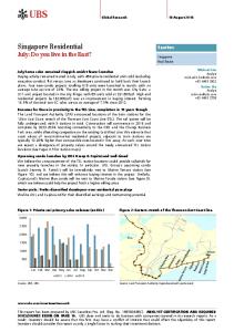
The wood has three main surfaces: 1) the cross-section surface; 2) tangential surface and; 3) radial surface, examples of these surfaces are shown in Figure 2.1. All three surfaces have different textures because cell structures vary when seen from different dimensions. Therefore the reference plane that 16
is being viewed must be determined in the first instances. The cross-section surface has the best characteristics to be observed and is often used for wood identification (Bond and Hamner, 2006).
Figure 2.1: Three surfaces of the wood (Bond and Hamner, 2006)
2.3.3 Structure of Wood
When a tree starts growing from the germinated seed, it forms a shoot known as the pith. The pith is surrounded by a thin meristematic tissue known as the cambium which itself is surrounded by the bark that protects it. During the growth, the division of the cambium cells happens. The cambium produces bark tissue on the outside which is known as the phloem and woody tissue on the inside which is known as the xylem.
17
During the growth, growth rings are produced when the cambium cells continue to expand and produce a new layer of wood between previously formed wood and the bark. In the temperate zone, vigorous growth happens in the early spring which gradually declines in vigor according to time. By late autumn, the growth will end. When growth starts again next spring, the clear contrast between the new vigorously growth cells with large and porous cells will be observable and this is the growth rings. Since it is grown each year, the calculation of the growth rings can be used to tell the age, and these growth rings are also known as annual rings. In tropical zone, the situation is different with the temperate zone where no distinct changes of seasons happen. Therefore, the growth rings do not happen yearly and usually do not have distinct differences in texture for two different layers of wood grown.
The woody parts of the trees are mainly used to transfer water and minerals from the roots to the leaves, store the reserved food materials and provide strength to the whole tree. The cells that do this within the woody part are known as the sapwood. As the tree grow outwards, the older wood in the inner part will be defunct and is known as the heartwood. The coloration of the heartwood and sapwood can be sharply contrasted with each other, such as rengas, kempas, keranji, merbau and etc. The coloration is same for both heartwood and sapwood in some other trees, such as jelutong, pulai, ramin, rubberwood and etc. The structures of the wood are illustrated in Figure 2.2 (Menon, 1993).
18
Figure 2.2: Structure of the wood (Menon, 1993)
2.3.3.1 Structural Features of Hardwood
The main features observable on the hardwood are vessels, wood parenchyma, ray parenchyma and fibers. Some other less common features are included phloem, latex traces and intercellular canals.
The vessels or pores are seen as small, round or oval holes in the wood. For the vessels, the perforation types, size and density, grouping and arrangement and contents are characteristics that are examined. The parenchyma tissue works as storage and distribution of reserve food materials. The vertical system is known as the wood parenchyma while the horizontal system is known as ray parenchyma or simply as rays. There are two major
19
types of wood parenchyma, namely the aprotracheal type which the cell or cell aggregates are typically independent of the vessels and paratracheal type which the cell or cell aggregates are closely associated with the vessels. The ray parenchyma or rays are lines grow from the pith to the bark of wood. In small cross-section surfaces, they appear to be horizontal and parallel. The width between the ray parenchyma is usually examined. The fibers are tissue that provides mechanical strength and rigidity to the wood. They are not significant to be observed but affect the weight and hardness of the wood due to the thickness of the cell walls.
Some other structural features are not common and may only appear in a few species. The included phloem is an abnormal behavior of the cambial sheath, wood structure may deviate from its normal position and phloem tissue gets included in the wood. This structure only appears in a few species of wood and is best seen in kempas and tualang. The latex traces or leaf traces are lens-shaped or slit-like passages running on the radial direction through the wood and is shown on the tangential section of the wood. One example of wood with latex traces is the jelutong. The intercellular canals are long and narrow passages, lined with a special type of parenchyma cells and are mainly used for secretion into the canals. These secretions vary in different type of wood, such as resin in chengal, oil in sepetir and gummy substances in kedondong. According to appearance, they are separated into vertical canals and horizontal canals (Menon, 1993).
20
2.3.3.2 Structural Features of Softwood
The main structures observable on the softwood is slightly different compared to the hardwood. The main features are the tracheids, wood parenchyma and rays. Other features include the intercellular canals and pitch pockets.
The tracheids form more than 90% of the softwood elements. They are long, tube-like cells with closed ends and numerous holes on the side walls. The growth rings are form when there is a noticeable difference formed between the tracheids formed during the early part and those formed before the resting period. Wood parenchyma in the softwood is similar to those found in the hardwood but the cells are comparatively sparse. The arrangement of the cells can be separated into diffuse, zonate and terminal. This structure is usually hard to be distinguishable with a hand lens. Rays in the softwood is also similar to those in the hardwood but the variation in the ray structure between species is insignificant and is usually regarded as useless in identification.
The intercellular canals in the softwood are also known as resin canals. They can be vertical or radial. They are surrounded by a special type of parenchyma which secretes into the canals to fill them with resin. The presence and the distribution of these canals are distinct and are helpful in the identification of softwood. The pitch pockets are abnormal openings or 21
pockets of variable size and shape in or between growth rings. These pockets contain resin and are thought to be formed due to injuries of the cambium during the growth of the tree, therefore are not helpful in identification of species (Menon, 1993).
2.3.3.3 Physical Features
The physical features are less important in wood species identification process, such as color, weight or density, hardness, texture, grain, figure and odor. However, it is sometimes helpful in species identification when combined with the structural features.
Color of the wood is hardly described because most of them are similar to each other and it also differs among the species itself for wood collected from trees from different geographical locations, age of tree and environment of growth. The weight and density differs for different species due to their different structures and will vary within species itself for differences on moisture level of the wood. The hardness of the wood also differs for different wood and is generally separated into four groups, i.e. very hard, hard, moderately hard and soft. The texture used to describe wood differs from the texture that is mentioned in texture classification, wood expert only examine if the texture of wood is fine, coarse, even or uneven. This information is often not significant in wood identification.
22
The grain of the wood is often mistaken as the texture of the wood, grain refers to the alignment of the longitudinal elements relative to the axis of the log, which includes straight, diagonal, spiral, interlocked, wavy and etc. The figures are patterns that are attractive and easily observable from the wood, such as growth ring, silver, stripe or streaky. The odor exists in certain species of wood, such as a spicy smell in medang and resinous smell in keruing. These usually stronger when the wood is freshly cut and will often fade or lost in the process of drying and exposure. Some other features such as burning characteristics and froth test can be examined (Menon, 1993).
2.3.4 Traditional Methods for Wood Identification
Wood experts usually identify the wood species by examining two different stages, first with the naked eye, then with a magnifier. With the naked eyes, the wood expert can observe the weight, color, feel, odor, hardness, texture and surface of the wood. This stage is to examine the physical characteristic that the wood species possess. With a magnifier, the wood expert will be able to observe and examine the anatomical features on the cross-section surface of the wood. A 10-time magnification hand lens is usually used. A sharp pocket knife is used to peel the surface of the wood to obtain a clear and smooth cross-section. The characteristics such as vessels and wood parenchyma are examined for hardwood. Softwood has no vessels and has insignificant wood parenchyma and rays, therefore the other
23
characteristics such as growth rings, resin canals and etc are examined for the identification purpose (Menon, 1993).
The anatomical identification process is the most important to identify the wood species. There are a few methods used to check which species the wood is through the characteristics observed under the macroscopic view such as visual comparison, dichotomous key and multiple entry keys.
2.3.4.1 Visual Comparison
Identifying species by comparing them are popularly used for many types of living things. Most field guides will illustrate similar species in a same section so that the user can use it to determine the species (Lew, 2005). The characteristics and anatomy of the wood are needed to compare with the information provided in the field guides. The problem of using such methods is that the comparison between similar species might be tedious when the differences are very small and very hard to be observed.
2.3.4.2 Dichotomous Key
The dichotomous key is another famous method used in identification of plants, wood, animals and etc. The dichotomous will provide a pair of keys
24
which are usually contrasting with each other at every level (Lew, 2005). Different keys will lead you to another pair of keys until the answer is found. 1A 1B
Vessels (pores) present Vessels (pores) absent
2A 2B
Vertical resin canals present Vertical resin canals absent
3 19
3A
Vessels moderately numerous or numerous (More than 10 per square mm) Vessels moderately few or few (Less than 10 per sq. mm)
4
3B
4A 4B
With ripple marks Without ripple marks
5A
With diffuse vertical canals: Rays of two distinct sizes Without diffuse vertical canals: Rays of single size only
5B
6A 6B
Wood hard or very hard Wood not hard or very hard
2 Damar Minyak
7
Chenggal 5 Resak 6
Giam Merawan
Figure 2.3: A small extraction from the dichotomous key for usage of those familiar with the anatomical features of timbers (Menon, 1993)
Dichotomous key is simple and easy to use but it will cause errors easily if the dichotomous keys have longer sequences. If any decision is wrong at the intermediate stage, then the results will be affected and the correct identification will not be achieved. Figure 2.3 shows a sample of dichotomous keys for wood identification.
25
2.3.4.3 Multiple Entry Keys
Since dichotomous keys can only provide two choices at every stage, errors will occur when the user gave the wrong answers at one of the stage as some characteristics are not easily observable. To solve the problem, multiple entry keys allows user to key in the characteristics without following any sequence. The chosen keys will then be used to compare with the data in the database to determine which species in the database has the most similar set of features.
Figure 2.4: A multiple entry keys example for some hardwood of Tennessee (Bond and Hamner, 2006)
However, there are still available implementations of multiple entry keys that can be drawn out as a tree which is similar to the dichotomous key 26
method as shown in Figure 2.4, which is a tree to determine the species of hard wood with possible choices which is more than two in some level.
2.3.5 Computer-based Methods for Wood Identification
Computers had been used to solve many real world problems, including wood recognition. Many previous works done are mainly based on the characteristics of the wood species provided by users and to match it with the information in the database to identify the species, this helps user to match characteristics in an automated way. Implementations of computer vision techniques are not popular yet for solving wood species identification problem.
2.3.5.1 Dichotomous and Multiple Entry Keys
Dichotomous keys and multiple entry keys are both depending on characteristics observed from the wood samples. Computerizations of such techniques are available on various websites such as MEKA system, FloraSearch (Lew, 2005) and FFPRI wood database. The multiple entry keys method is more popular since the user can enter all information for the characteristics that they observed without worrying that the mistakes done during the intermediate stages of dichotomous keys method will produce a wrong answer. A sample screen on the interface of FFPRI microscopic database is shown in Figure 2.5.
27
Figure 2.5: Sample screen of graphical user interface of FFPRI microscopic database for wood identification (http://f030091.ffpri.affrc.go.jp/index-E3.html)
2.3.5.2 Vision Technology
Earlier work are mainly focusing on the grading of wood and the detection of detect units. Ultrasound, microwave, nuclear magnetic resonance, X-ray technologies, laser ranging, cameras and spectrometers are used in vision technology. Recently, a tropical wood recognition system called KenalKayu is developed which is a system that uses the GLCM as the feature extractor and an MLP as the classifier. The recognition rate is 90.81% and it is tested on 20 species of wood (Lew, 2005).
28
2.4 Embedded Systems
Generally embedded system differs from general-purpose computers in terms of the user interface. We are familiar with the monitor, keyboard, and mouse to control and navigate the computer. An embedded system may not have a user interface, or it can have a touch screen, a button and etc (Lombardo, 2002). Even the handheld computers and PDAs fall in this category as embedded systems.
Embedded systems have the benefit of being lighter in many cases and it is also more transportable from one location to another. Embedded system can be a mobile device to be brought into the needed environment; they can also be placed at a fixed location such as for traffic surveillance. For the example on traffic surveillance, the system is able to detect vehicles and their license plate (Arth et al., 2006).
Although embedded systems can provide good mobility and is able to perform a specific task, the embedded system often suffers the problem of having limited processing power, resources and space. All of these have to be taken into consideration during the development of an embedded system; the codes must be as optimal as possible to ensure the speed of processing and the accuracy of the results are desirable.
29
2.5 Summary
This chapter introduces textures and the main categories of texture classification techniques that are being used. The structures and characteristics are discussed along with wood identification techniques that are used. Earlier methods uses the anatomical characteristics as the main criteria to determine the species while more recent techniques including computer vision can rely on the texture of the wood cross-section surface. The embedded systems are also briefly introduced.
30
CHAPTER 3.0
DESIGN OF SOFTWARE FOR TEXTURE CLASSIFICATION
3.1 Introduction
This chapter includes the overall software architecture of the texture classification system using grey level co-occurrence matrices (GLCM), Gabor filters and covariance matrix together with multi-layer perceptron (MLP) and k-NN as the classifiers. The offline system uses 32 Brodatz textures and CAIRO wood dataset for evaluation purpose. For the online system, the images are live captured using a camera. The details of each process will be described in the following parts of the chapter.
3.2 Software Architecture
The system includes a few important components. i.e. image acquisition, pre-processing, feature extraction and classification. There are two major phases, which is the training phase and testing phase. First a set of data will be used for the training phase and another set will be used for the testing phase.
The system starts with an image acquisition process where the input samples are captured using a camera. After the input image is captured, it will 31
be normalized through the pre-processing process. The normalized input will be used for feature extraction where the important textural features are extracted here. The extracted features will be classified using a classifier and produces an output as shown in Figure 3.1.
Figure 3.1: The architecture of the texture classification system
For the development of the whole system, a dataset is first collected to be used for the training and testing of the system. Half of the dataset is selected for the training process where the features extracted from these samples are used to train the classifier. The other half of the data is used for testing and evaluation of the system. After training and testing the system on the offline module, the same process will be done on the online module where the input images are captured using the camera.
32
3.3 Image Pre-processing
Pre-processing are processes applied on the input images in order to eliminate anomalies and noise or to further enhance certain details of the image for better recognition. The goal of pre-processing is to enhance the images so that characteristics which will help in the recognition process are obtained. The pre-processing that is performed in this thesis is histogram equalization.
3.3.1 Histogram Equalization
Histogram equalization is used to enhance the contrast of the images. The normalization of the intensity distribution will reduce the impact of different illumination applied on the images especially for images taken under bright or dark conditions.
The probability density function (PDF) is used to achieve histogram equalization. The probability of occurrences of grey level p(xi) is represented in Equation (3.1) where ni represents the number of occurrence for grey level of i, n represents the total number of pixels in the image, and G represents the number of grey levels in the image.
p(xi) =
ni n
where i 0,1,2,…,G - 1
(3.1)
33
Then the cumulative distribution function (CDF) ci is represented in Equation (3.2).
i
where i 0,1,2,…,G - 1
ci = ∑ p(xj)
(3.2)
j=0
The output image after histogram equalization is produced by mapping each pixel with level p(xi) in the input image into the corresponding level ci onto the output image oi using Equation (3.3) (Gonzalez and Woods, 2002).
G-1
oi = ∑ ci (G - 1)
(3.3)
i=0
3.4 Feature Extraction
Feature extraction is an important process in the texture classification as it extracts a numbers of values from the input images through various image processing algorithms. This process reduces the input values by ignoring the raw pixel values of the whole input images and focus only on useful values that represents the features or properties of the image. For an ideal situation, samples from the same class should be providing similar feature values, this is however not always true especially for input samples that are not considered to be homogeneous.
34
In this thesis, a few feature extraction algorithms that are commonly used for texture classification is studied and used. The algorithms are GLCM, Gabor filters and covariance matrix. The techniques will be further discussed in the following sub-sections.
3.4.1 Grey Level Co-occurrence Matrices (GLCM)
The GLCM is generated by cumulating the total numbers of grey pixel pairs from the images. To generate a GLCM, there are four orientations that could be focused on during the generation of the matrix, which are 0° (or horizontal) direction, 45° direction, 90° (or vertical) direction, and 135° direction as shown in Figure 3.2 and a spatial distance which represents the number of pixels between the reference pixel r and the neighboring pixel n. The orientation and spatial distance is represented by d.
Figure 3.2: Four orientations for generation of GLCM
35
The number of grey level G can be selected to generate the GLCMs, the produced matrices will be the size of G × G. A normal grey-scaled image will have 256 values, ranging from 0 to 255. If a selected G is less than 256, therefore, the image will be normalized to reduce the number of values to G.
As shown in Figure 3.3, the two matrices at the left represents two different sample images while the two matrices at the right are respective GLCM generated where d is defined to be 1 pixel and orientations which are stated in the figure. For the GLCMs, the vertical axis represents the reference pixels and the horizontal axis represents the neighboring pixels. To calculate the values in the GLCM, it is the total number of occurrence for the certain reference and neighboring pixels pair for d. The G is selected to be 5 for the examples which are the values of 1 to 5 in the figure in order to show a simple generation of the GLCMs. For the example on top, the orientation is 0 degree and the spatial distance is 1 pixel, therefore it could be calculated that the count for reference pixel with grey value of “1” with adjacent pixel with grey value of “1” is 2 and 1 for adjacent pixel with grey value of “3”, and so on. For the lower example, the orientation is 45 degree and d is the same, e.g. the count of reference pixel with grey value of “5” where the adjacent pixel for 45 degrees with grey value of “2” is 2. Many GLCMs with different orientations and spatial distances could be generated to solve a particular problem.
36
Figure 3.3: Example of generating GLCMs
When the GLCM is constructed, Cd(r,n) represents the total pixel pair value where r represents the reference pixel value and n represents the neighboring pixel value according to the spatial distance and orientation defined. Cd represents the total number of pixels in the image. The joint probability density function normalizes the GLCM by dividing every set of pixel pairs with the total number of pixel pairs used and is represented using p(r,n) as shown in Equation (3.4) (Petrou and Sevilla, 2006).
p(r,n) =
1 Cd
Cd(r,n)
(3.4)
37
When the GLCM is generated, there are a total of fourteen features that could be computed from the GLCMs, such as contrast, variance, sum average, and etc. The five common textural features discussed here are contrast, correlation, energy, homogeneity, and entropy. Contrast is used to measure the local variations, correlation is used to measure probability of occurrence for a pair of specific pixels, energy is also known as uniformity of angular second moment (ASM) which is the sum of squared elements from the GLCM, homogeneity is to measure the distribution of elements in the GLCM with respect to the diagonal, and entropy measures the statistical randomness. The 5 common textural features are shown in Equation (3.5) to (3.13) (Petrou and Sevilla, 2006).
Energy:
Entropy:
Contrast:
G-1
G-1
r=0
n=0
G-1
G-1
r=0
n=0
∑ p(r,n)2
∑ ∑
∑ -p(r,n) log p(r,n)
1
G-1
G-1
(G–1)2
r=0
n=0
G-1
Correlation:
(3.5)
∑ r=0
∑
∑ (r – n)2 p(r,n)
(3.6)
(3.7)
G-1
∑ rn p(r,n) - xy
n=0
(3.8)
xy where
x = y = x = y =
G-1
G-1
∑r
∑ p(r,n)
r=0
n=0
G-1
G-1
∑n
∑ p(r,n)
n=0
r=0
G-1
∑ (r – x)2
∑ p(r,n) n=0
G-1
G-1
n=0
(3.10)
G-1
r=0
∑ (n – y)2
(3.9)
∑ p(r,n)
(3.11)
(3.12)
r=0
38
G-1
Homogeneity:
p(r,n)
G-1
∑ ∑
r=0 n=0
(3.13)
(1 + |r – n|)
3.4.1.1 One-dimensional GLCM
To reduce computations, the GLCM dimension can be reduced from two dimensions to one dimension by combining certain values of the matrix. By focusing only on the differences of the grey level, we are only concerning on a one-dimensional GLCM with a significantly smaller size which is only 2 × G - 1, compared to G × G for a conventional two-dimensional GLCM. By reducing the dimension of the GLCM, the calculations of features will be faster as fewer values are involved in the calculation.
For the one-dimensional GLCM, the joint probability density function p(x) is similar, but focuses only on the differences of grey value between the pixel pairs, where x shows the differences of grey value and Cd(x) shows the total number of pixel pair with x, as shown in Equation (3.14).
p(x) =
1 Cd
Cd(x)
(3.14)
The feature formulas are modified to suite the one-dimensional GLCM, this is done as the original feature extraction functions involved two dimensional data from the GLCM as shown in 3.4.1. The correlation feature of 39
the conventional GLCM is omitted as it involves the calculations of specific pixel pairs, but the one-dimensional GLCM has merged a few pixel pairs with the same grey differences into one, therefore has lost the information for specific pixel pairs.
For the modification of the textural features, the summation function that involves every value in the GLCM is only one dimension in the onedimensional GLCM, and the joint probability density p(m,n) is replaced by p(x) in the one-dimensional GLCM. The calculation of (r-n) that represents the differences of grey value in the conventional GLCM is represented by x that represents the same thing in the one-dimensional GLCM. After the modification, the values of contrast and homogeneity will be identical but the values of energy and entropy will be different with the conventional GLCM. The modified features are shown below from Equation (3.15) to (3.18).
G-1
Energy:
∑
p(x)2
(3.15)
-p(x) log p(x)
(3.16)
m=-(G-1) G-1
Entropy:
∑
m=-(G-1)
1 Contrast:
(G – 1)2 G-1
Homogeneity:
∑
m=-(G-1)
G-1
∑ (x)2 p(x)
(3.17)
m=-(G-1)
p(x) (1 + |x|)
(3.18)
40
3.4.2 Gabor Filters
The Gabor filters, also known as Gabor wavelets, is inspired by the concept of mammalian simple cortical cells (Yap et al., 2007).
The Gabor filters is represented by Equation (3.19) where x and y represent the pixel position in the spatial domain, w0 represents the radial center frequency, represents the orientation of the Gabor filter, and represents the standard deviation of the Gaussian function along the x- and yaxes where x = y = (Yap et al., 2007).
x, y , 0 ,
1 2
e
2
2 2 2 e x cos y sin x sin y cos / 2
i 0 x cos 0 y sin
e
02 2 / 2
(3.19)
The Gabor filter can be decomposed into two different equations, one to represent the real part and another to represent the imaginary part as shown in Equation (3.20) and Equation (3.21) respectively (Yap et al., 2007) and in Figure 3.4. x 2 y 2 02 2 r x, y, 0 , exp 2 cos 0 x exp 2 2 2 1
i x, y , 0 ,
x 2 y 2 sin 0 x exp 2 2 2 1
(3.20)
(3.21)
41
where x' = x cos + y sin
y' = -x sin + y cos
Figure 3.4: Real part (left) and imaginary part (right) of a Gabor filter (Nixon and Aguado, 2002)
In this thesis, we used = / w0. Gabor features are derived from the convolution of the Gabor filter and image I as shown in Equation (3.22) (Yap et al., 2007). CI = I(x, y) * (x, y, w0, )
(3.22)
The term (x, y, w0, ) of Equation (3.22) can be replaced by Equation (3.20) and Equation (3.21) to derive the real and imaginary parts of Equation (3.19) and is represented by CIr and CIi respectively. The real and imaginary parts are used to compute the local properties of the image using Equation (3.23) (Yap et al., 2007). CI(x,y,w0,) = √ ||CIr||2 + ||CIi||2
(3.23) 42
The convolution can be performed using a fast method by applying fast Fourier transform (FFT), point-to-point multiplication and inverse fast Fourier transform (IFFT). This method is to reduce the computations comparing to conventional method which used a smaller subwindow to perform convolution over the whole image. It is performed on three radial center frequencies or scales, w0 and eight orientations, . In this thesis, the radial center frequencies and orientations are represented by wn and m respectively in Equation (3.24) where n {0, 1, 2} and m {0, 1, 2, …, 7} (Yap et al., 2007).
wn =
2(2)n/2
m =
8
m
(3.24)
3.4.2.1 Reducing Dimensionality for Gabor Features
The Gabor features are at a high-dimensional space. The high dimension of the feature space will cause difficulty in the classification of the problem. A down-sampling can be performed by omitting values from the Gabor features with a factor of . The Gabor features are concatenated to form a feature vector as shown in Equation (3.25) (Yap et al., 2007). C() = (CI()(x,y,w01,1), CI()(x,y,w01,2),…, CI()(x,y,w01,m),…, CI()(x,y,w0n,m))T
(3.25)
A principal component analysis (PCA) can be performed to further decompose the Gabor feature size. Singular value decomposition (SVD) can
43
be performed for a faster method of decomposing the feature vector. The SVD decomposes an i × j matrix C into three matrices as shown in Equation (3.26). C = u × × vT
(3.26)
where p is the minimum of i and j, u is a matrix of dimension i × k, is a matrix of dimension k × k , v is a matrix of dimension j × p (Klema and Laub, 1980).
A feature size s is selected to decompose the matrix u from m × k to an m × s matrix by directly discarding the values from the matrix beyond the size to obtain . The final Gabor feature matrix after the decomposition is shown in Equation (3.27) (Yap et al., 2007). () = T (C() - )
(3.27)
3.4.3 Covariance Matrix
A covariance matrix shows the covariance between values. In this thesis, the fast covariance matrix calculation using integral images that is proposed by Tuzel et al. (2006) to generate the covariance between different feature images is used as the features for our algorithm. The feature images are a set of two-dimensional images or matrices obtained from the original image after implementing some image processing or feature extraction algorithms on it. 44
The covariance matrix can be represented as
CR
1 n z k z k T n 1 k 1
(3.28)
where z represents the feature point and represents the mean of the feature points for n feature points (Tuzel et al., 2006).
Integral images are used for faster computation. The summations for each pixel of the image from the origin point are pre-calculated. This will fasten the process of acquiring the sum for a region within the images with simple calculations. The calculations of the term P and Q which are two tensors for the fast calculation of the covariance matrix are shown below:
Px, y, i
F x, y, i
i 1...d
x x, y y
Qx, y , i, j
F x, y, i F x, y, i
i, j 1...d
x x , y y
(3.29)
(3.30)
where F represents the feature images and d represents the dimension of covariance matrix which is also the number of feature images.
The covariance matrix is then generated using P and Q where x, y is the upper left coordinate and x, y is the lower right coordinate of the region of interest as below (Tuzel et al., 2006):
45
C R x, y; x, y
1 Qx, y Qx, y Qx, y Qx, y n 1
1 T Px, y Px, y Px, y Px, y Px, y Px, y Px, y Px, y n
(3.31)
3.4.4 Feature Normalization
Feature normalization normalizes the features so that each feature will have value range that is similar so that it will not be biased towards features with greater value in the image. This avoids the performance of the classifier to be affected by certain features due to value range.
The normalization process sorts the feature values to construct a distribution graph and chooses the value at 1% and 99% as the minimum and maximum value respectively. The absolute maximum and minimum is not chosen to avoid the presence of outliers. The normalized features N(x) is shown in Equation (3.32) where x represents the original feature values, Fmin represents the minimum feature value and Fmax represents the maximum feature value (Lew, 2005).
N(x) =
x - Fmin Fmax – Fmin
(3.32)
46
3.5 Classification
Classifiers are used to classify the problem using the features extracted from the feature extraction step. They will produce an output to tell which class the testing samples should fall under. Classifiers implemented in this thesis include k-NN, and MLP.
3.5.1 k-Nearest Neighbor (k-NN)
The k-NN is a simple adaptive kernel method. It stores the features of a set of training samples, and it compares a test sample with all the available training samples and chooses the k training samples that are nearest to the test sample. The class with highest number chosen within the k training samples will be the winning class for the test sample. The 1-nn is often rather successful (Ripley, 1996). The Euclidean distance is used to compare between samples and the smaller distances show that the samples are nearer to each other (Perlovsky, 2001).
The method requires comparison with all training samples, therefore it will be slower if the training set is larger, but will affect the results if the training set is not large enough. On the other hand, if the training samples are large, it consumes storage space on the computer.
47
3.5.1 Distance Calculation for Covariance Matrix
The covariance matrix does not lie on the Euclidean space, so the Euclidean distance is not suitable to be used as the metrics calculation for the distance. The metrics calculation that is adopted here is using the generalized eigenvalues which is first proposed by Forstner and Moonen (1999):
C1 , C2
n
ln C , C 2
i 1
i
1
2
(3.33)
where i(C1,C2) represents the generalized eigenvalues of C1 and C2 that are computed from
iC1 xi C2 xi 0
i 1...d
(3.34)
where xi ≠ 0 (Tuzel et al., 2006).
3.5.2 Multi-layer Perceptron (MLP)
The MLP is a common supervised neural network that is used as the classifier for many different pattern recognition problems. A neural network imitates a biological neural system which is grouped up by a number of neurons so that they can learn a certain task. MLP is a design which is simple yet powerful and has proven to be useful in many different applications. The main idea of the MLP is to allow the neural network to learn through the given training samples and is able to predict and tell that a similar but not identical input against a training input that belongs to the same class (Fausett, 1994). 48
The neurons are the simplest unit in an MLP. Each neuron can take in one or more input values, which will be sum up using the dot products of the input values and their respective weights which is represented by ∑wixi, where w represents the weights of each input x for i {0, 1, 2, …, n} and n represents the number of input. This sum will be computed through an activation function to produce the output of the neuron. A bias is often added as an extra input where the input value remains to be constant. The structure of a neuron is shown in Fig 3.5.
Figure 3.5: Structure of a neuron
Activation functions f(x) that are commonly used include the threshold, linear, sigmoid and hyperbolic tangent function. The threshold function has two possible outputs determine by a threshold value of c as shown in Equation (3.35).
f(x) = {
1, x ≥ c 0, x < c
(3.35)
49
The linear function has the same output as the input shown in Equation (3.36). f(x) = x
(3.36)
The sigmoid and hyperbolic tangent functions are widely used. They have continuity of the function over its range of value, the sigmoid function has a range of (0,1) while the hyperbolic tangent function has a range of (-1,1) as shown in Equation (3.37) and (3.38) respectively.
f(x) =
1 1 + e-x
f(x) = tanh(x) =
1 – e-2x 1 + e-2x
(3.37)
(3.38)
The softmax function is an activation function with the output value range of (0,1) and all the output values of the output layer is sum up to 1. This activation function is often used in the output layer of the MLP to show probabilities as shown in Equation (3.39).
f(xj) =
e xj ∑ e xi
(3.39)
i
An MLP is formed by layers of neurons. A simple MLP has an input layer, a hidden layer and an output layer. The input layer gets the input with 50
no activation function and sends the values to the hidden layer, where the hidden layer will process the value with an activation function and send the calculated value to the output layer where a similar process is done and produced the output. There can be more than one hidden layer in an MLP. The structure of an MLP is shown in Fig 3.6.
Figure 3.6: Structure of an MLP
3.5.2.1 Back-propagation (BP) Learning
The BP algorithm is a learning algorithm used for training the MLP. It resembles the learning of a human brain, where training samples are fed into the MLP with their respective teaching signals. If the output does not match, BP algorithm will be performed to update the weights from the output layers towards the input layer; therefore it is known to be a back-propagation.
51
During the initial stage, the MLP is initialized with random weights; the weights are initialized at a certain range to avoid bias of certain values if their initialized weights are far greater than the rest. After initialization of the weights, the MLP will go through a BP learning process that involves the looping of the following steps.
First, input of a training sample will be fed into the MLP for a forward propagation to obtain an output value using Equation (3.40) and Equation (3.41) where x represents the net inputs of each neuron, y represents the output and wji represents the weights from the ith neuron to jth neuron of the next layer. xj = ∑wjiyi i
(3.40)
yj = f(xj)
(3.41)
Then a comparison will be made with the respective teaching signal and update the MLP by first checking the error for each layer using Equation (3.42) and Equation (3.43) for output layer and hidden layers respectively where represent the errors, t represents the teaching signals, k and h represents the neurons of the output and hidden layers respectively.
k = yk(1 - yk)( tk - yk)
(3.42)
h = yh(1 – yh) ∑ wkhk
(3.43)
k
52
After the calculations of the errors for each layer, the weights are updated according to Equation (3.44) where wji’ represents the updated weights and represents the learning rate. wji’ = wji + kyji
(3.44)
The number of training epochs is determined by the criteria for stopping the neural network. The sum of squared error (SSE) is a common criteria used to determine when to stop the training process of a neural network which is shown in Equation (3.45) where p represents the layers of the neural network.
1 E=
2
∑ ∑ (tk - yk)2
(3.45)
p k
The training process will stop when the SSE converges where it no longer decreases. The learning rate will decrease for each training epochs to reduce the impact of learning to the neural network so that the learning will slow down. The training samples should be randomly fed in to avoid over training so the neural network to a certain class of training samples (Lew, 2005).
53
3.6 Verification-based Recognition
A verification process can be added prior to the recognition process. The method will first use the verification algorithm to decide if the test samples are of the same class with each of the templates provided and decide which class it should belong to.
3.6.1 Feature Extraction for Verification-based Recognition
First, we calculate the features from the training template. In this thesis, the GLCM and covariance matrix are used as the features. For the GLCM, four GLCMs are generated for each sample and the raw GLCMs are directly used as features without calculating the second-order features from the GLCMs. For the covariance matrix, twelve Gabor filters of four orientations and three radial center of frequencies are used to produce the feature images for the generation of the covariance matrix. These feature vectors are stored as templates.
The features are then calculated for the test, but for eight different orientations of the image. Instead of rotating the images for eight different orientations, we remain the images while changing the orientations during the calculations of the features. Eight directions are calculated to select the rotation angle that provides the closest feature comparing to the templates since the images obtained might not be of a same direction. The angle 54
difference between each direction is 45°. Since the Gabor filters has no directions for each of their orientations, there are only four possible sets of directions that can be generated for four orientations. The rotation of direction selection for the GLCMs and Gabor filters are shown in Figure 3.7 and 3.8 respectively.
Figure 3.7: Eight directions of the GLCMs
Figure 3.8: Four directions of the Gabor filters
By studying eight different directions, the test sample can be rotated to the nearest direction with the templates. This can reduce the anomalies caused by differences in directions and hence achieve rotational invariant for the algorithm.
55
3.6.2 Verification Process
The verification process involves the algorithm to verify whether the tested sample is from the same class with the samples in the templates. This process is accomplished by first comparing the test sample with the templates and decides whether they belong to a same class.
First, for the training module, to calculate the similarity of two samples, the energy E’ of the difference between the two feature vectors is calculated as shown in Equation (3.46) where n represents the number of features, f’ represents the feature vector the templates, t represents the number of templates, x ϵ [1,t] and y ϵ [1,t]. n
E ( x, y ) ( f x(i) f y (i)) 2
(3.46)
i 1
For the covariance matrix, the metric calculation used is proposed by Forstner and Moonen (1999) because it does not fall in the Euclidean space as shown in Section 3.5.1. The adapted equations are shown in Equation (3.47) and (3.48).
E ( x, y)
ln f (i), f (i) n
2
i 1
i
x
y
(3.47)
56
where i represents the generalized eigenvalues of two feature vectors.
i f x(i) xi f y (i) xi 0
i 1...d
(3.48)
The threshold T is generated for each template according to class using Equation (3.49) where represents the mean for each class, represents the standard deviation for each class, s represents the number of templates for the class, and x ϵ [1,s]. For the covariance matrix, Equation (3.50) is used instead.
1 T x x E x x E x 2
(3.49)
1 T x x E x x E x 2
(3.50)
After the threshold value is obtained, the energy E of the difference between the feature vectors of the test sample and the template is calculated as shown in Equation (3.51) where n represents the number of features, f’ represents the feature vector template, f represents the feature vector of the test sample and f represents the orientation of the test sample. n
E i 1
min ( f (i) f (i))
2
(3.51)
0...360
57
If a test sample is having E less than Ti, they will be accepted as the same class with the ith template. The selection threshold is lower than the mean for each class; therefore it reduces the possibility of accepting false samples but will reject correct samples which are slightly more different than the templates.
3.6.3 Recognition Process
For each test sample, the verification process will be conducted by testing it against all the templates. The class with the highest accepted templates will be selected as the winning class for the particular test sample.
3.7 Summary
This chapter introduces every step of the system architectural design from the pre-processing to the classification stage in details. The preprocessing stage involves the histogram equalization. The feature extraction stage is extensively described for the GLCM, Gabor filters and covariance matrix which are the main techniques used in this thesis. The classifier explained includes the artificial neural network and k-NN which are used in the experiments. Finally a last section introduces the verification algorithm that can also be extended for recognition purpose which is also used in this thesis.
58
CHAPTER 4.0
INTEGRATION OF ALGORITHM ONTO EMBEDDED PLATFORM
4.1 Introduction to Embedded Devices
Embedded devices are becoming popular due to their small sizes that often promote mobility. In order to embed an algorithm onto an embedded platform, the size and computational steps of the algorithm has to be taken into consideration. Embedded platforms are usually less powerful than personal computers due to their small sizes. They often offer slower processors and smaller memory capacity, therefore an algorithm usually run much slower in an embedded platform that is less powerful. Integrating the texture classification algorithm especially wood species recognition algorithm into the embedded platform provides a few advantages, especially in mobility, simplicity of the system and etc.
4.2 Process for Embedding
In order to embed the texture classification system, there are a few basic steps to be done. First, the algorithm is developed and tested using methods described in the previous chapter. The algorithm will be first tested on an offline dataset to fine tune the algorithm to produce better results. After the algorithm is well examined using the offline datasets, the algorithm will be fed with online inputs. When the online algorithm is tested, it should be 59
converted into codes to be deployed onto the embedded board. The process is shown in Figure 4.1.
Figure 4.1: Process of embedding the texture classification system
4.3 Online Personal Computer-based System
Before deploying the system onto the embedded platform, the system is developed and tested on the personal computers (PC). The system uses an acquisition device platform attached to the personal computer. The setup of the system is shown in Figure 4.2.
Figure 4.2: Setup of the online PC-based system
60
4.3.1 Image Acquisition for PC-based System
For the capturing of image, the acquisition device consists of a stand to stabilize the camera, an industrial camera and a light source. The industrial camera model is DNV 2001 that has a resolution of 1280 × 1024 pixels. The light source that is used here is a red colored ring light, the red colored light is selected because it is more economical and the images will be greyscaled.
The industrial camera consists of the camera itself, an extension tube and the camera lens. The extension tube is used to extend the focal length of the camera. The camera set is shown in Figure 4.3.
Figure 4.3: Acquisition Device
61
4.3.2 Development Tools
The prototypic system is developed using Simulink for rapid and simple development. The Simulink is also selected due to the capability of using the Real-Time Workshop to convert Simulink models into C programming codes that can be deployed onto the embedded platform. However, for the Real-Time Workshop, most of the MATLAB functions are not supported for the conversion into C programming codes, the functions have to be rewritten in order to perform the conversion.
4.4 Embedded System Architecture
For the purpose of wood species recognition, the embedded system includes a few components. A processing board is the processor for the system that processes the images, calculates the feature and classifies them. A camera is needed for the acquisition of input image.
The processing board that is used here is an Embedded Computer Vision (ECV) platform developed using the ARM processing board for embedding computer vision systems onto the platform. The ARM processor is running on the Linux operating system which is a Debian Linux distribution using the Linux 2.6 kernel. A VGA webcam with a resolution of 320 × 240 pixels is used for the platform. For the prototype, there is no display device included on the prototype and there are no control buttons to control the board, 62
therefore the input and output communications are achieved using a PC desktop through the network. The setting of the ECV platform is as shown in Figure 4.4.
Figure 4.4: Setup of the ECV platform
There are two models of ARM processing boards that are used in this thesis which are the ARM920T and ARM926EJ-S. The ARM920T has a Cirrus Logic EP9315 200MHz processor while the ARM926EJ-S has a Digi International NS9750B 200 MHz processor. Both models have 64 MB of RAM and 2 GB of harddisk space.
Due to the lack of available drivers for instant plug-ins, the acquisition device used for the ECV platform is not the same as the industrial camera used in the PC-platform. For the final implementation, the training process has to be 63
conducted on images captured using the same capturing device under the same lighting conditions.
4.4.1 Exporting Codes to ECV Platform
For fast development of embedded systems, the system is developed using Simulink that is using a fast model based development method. The Simulink blocksets will be converted into ANSI C using the Real-time Workshop but all blocksets must be supported, many MATLAB functions are not supported to be converted by Real-time Workshop.
The GLCM and k-NN functions used in this system is not supported by Real-time Workshop, therefore an Embedded MATLAB function is written for these functions and are tested against the MATLAB functions to ensure the outcome of both functions are identical to each other. The generated ANSI C will be exported to the ECV board and minor modification and respective libraries have to be added to make the system run on the ECV platform.
Due to the complexity of the algorithms involved, the direct conversion to ANSI C is difficult to be modified for the use in the ECV platform. Therefore a faster solution is often to rewrite the codes using ANSI C codes directly and to verify the generated results for each stage against the MATLAB and Simulink implementation. 64
4.5 Summary
This chapter introduces the integration of the algorithm onto the embedded platform. The steps to perform such integration are described including the offline experiments, online experiments and the transition from the PC platform to the ECV platform. The development tools that are needed during the transition and the specification of the ECV platform are also introduced.
65
CHAPTER 5.0
EXPERIMENTS AND ANALYSIS
5.1 Introduction
This chapter includes the experimental materials and settings used in the experiments, such as dataset, tools and neural network settings. There are four main phases of experiments conducted in this thesis. An evaluation of the speed on the embedded platform is also conducted to select the best algorithm for deployment into the embedded platform.
5.2 Experimental Materials and Settings
A few materials and settings for the experiment are used throughout all experiments, including the dataset, tools and neural networks used. Features are not normalized for the implementation unless it is otherwise addressed.
5.2.1 Experimental Datasets
The datasets used for the experiments include part of the Brodatz texture dataset (Brodatz, 1996), as used in the work of Valkealahti et al. (1998) and Ojala et al. (Ojala et al., 1999) (Ojala et al., 2001). 32 textures from the entire Brodatz texture dataset which includes a total of 112 textures (Picard et 66
al., 1993) are used here for the experiments. Each texture is separated into 16 equal size samples, each of these samples have four variants, the original image, the rotated image, the scaled image and the image that is both scaled and rotated. 8 original images and their variants are randomly selected as training set for each texture and the rest as testing set. Therefore there are a total of 1024 training samples and 1024 testing samples (Valkealahti et al., 1998).
For the wood dataset, the CAIRO wood dataset obtained from Centre for Artificial Intelligence and Robotics (CAIRO), Universiti Teknologi Malaysia (UTM), Malaysia, and the FFPRI wood dataset from Forestry and Forest Products Research Institute (FFPRI), Japan. The CAIRO wood dataset consist of macroscopic view of wood samples. There are three different subsets selected from the CAIRO dataset are used in different experiments below that will be further explained in the respective sections.
For the FFPRI dataset, there are 10 microscopic images for each of the 20 species. 10 samples of the size of 250 × 450 pixels are cropped from the microscopic images, producing 100 samples for each of the species. The 50 samples obtained from the first 5 images are used as training set while the next 50 samples obtained from the other 5 images are used as testing set for the each species. Hence, there are a total of 1000 training samples and 1000 testing samples. The 20 species of wood that are selected from the FFPRI dataset for the experiments are: 67
1. Acanthopanax sciadophylloides
11. Clethra barvinervis
2. Acer carpinifolium
12. Cornus controversa
3. Actinidia arguta
13. Daphniphyllum teijsmannii
4. Alnus hirsuta
14. Elliottia paniculata
5. Aralia elata
15. Euonymus oxyphyllus
6. Aucuba japonica
16. Ilex crenata
7. Benthamidia japonica
17. Lyonia ovalifolia
8. Betula grossa
18. Pieris japonica
9. Carpinus japonica
19. Rhododendron dilatatum
10. Cercidiphyllum japonicum
20. Rhus trichocarpa
5.2.2 Experimental Tools
The main tool used for the experiments is MATLAB (R2006b), with three toolboxes used, including the Image Processing Toolbox for reading images and GLCM computations, Neural Network Toolbox for neural networks and Bioinformatics Toolbox for k-NN.
5.2.3 Neural Network Settings
The neural networks that are used in the experiments are MLPs created using the Neural Network Toolbox. The functions of the neural network are shown in Table 5.1 and the training parameters in Table 5.2.
68
Table 5.1: Functions of the neural networks Functions training function adaption learning function performance function transfer function (hidden layer) transfer function (output layer)
Value
Description Levenberg-Marquardt TRAINLM backpropagation Gradient descent with LEARNGDM momentum weight and bias MSE Mean squared error TANSIG
Hyperbolic tangent sigmoid
SOFTMAX
Softmax function
Table 5.2: Training parameters of the neural networks Training Parameters Maximum number of epochs to train Performance goal Minimum performance gradient Initial mu mu decrease factor mu increase factor Maximum mu
MATLAB Parameters
Value
epochs
100
goal min_grad mu mu_dec mu_inc mu_max
0 1 × 10⁻¹⁰ 0.001 0.1 10 10000000000
The mu is adaptive and it increases by the mu increase factor until there is a reduction in the performance value. The weights of the neural network will be updated and the mu will decrease by the mu decrease factor.
The training stops when one of the criteria below is met: 1. Achieved maximum number of epochs to train. 2. Performance is minimized to the performance goal.
69
3. Performance gradient is minimized to the minimum performance gradient. 4. The mu exceeds the maximum mu.
5.3 Experimental Phases
The experiments are conducted in four main phases. The first phase is to test the features and GLCM method with a small wood dataset. The second phase test on more samples for each species as well as more species. The third phase is the main experiments run on the texture dataset with various algorithms. The last phase is to test the verification-based recognition algorithm on wood species recognition and compared it against other texture classification techniques.
5.4 Experiment Phase 1
The first experiments are only conducted a total of 50 wood samples in order to check the usefulness of the texture classification algorithms and to perform an analysis on the features selected.
There are 5 species of wood selected from the CAIRO dataset with 10 samples each, where the first 5 is used for training and the other 5 is used for
70
testing. There are a total of 25 samples for training and 25 samples for testing. The 5 species are: 1. Terentang (Campnosperma auriculatum) 2. Jelutong (Dyera costulata) 3. Durian (Durio lowianus) 4. Mata Ulat (Kokoona littoralis) 5. Mersawa (Anisoptera costata)
5.4.1 Analysis on GLCM Features
The analysis on the values of the GLCM features is performed to study the usefulness of the feature to discriminate the species and the suitable parameters to be used for obtaining a better set of GLCM features. The GLCM features are obtained from the input images, the five common feature functions are tested on two species of wood, which are Terentang (Campnosperma auriculatum) and Jelutong (Dyera costulata), with ten images for each species. The feature functions are contrast, correlation, energy, entropy, and homogeneity. The experiments are run on all four directions with spatial distance from 1 to 20 pixels. All of these analysis and experiments are run on images which are not enhanced through image processing.
The experimental results show that the values differ in all spatial distances for energy as shown in Figure 5.1 and Figure 5.2 where the vertical
71
axis represents the value of energy and the horizontal axis represents the value of spatial distance, but the graphs are shown in a similar pattern, therefore the pattern of change for energy may be useful as a feature to be extracted. However, although the value shows some difference within a certain species, the range of values still allows the feature to be useful for classification of the species.
Figure 5.1: Energy on 0° for Terentang (Campnosperma auriculatum)
Figure 5.2: Energy on 0° for Jelutong (Dyera costulata)
72
Figure 5.3: Contrast on 90° for Terentang (Campnosperma auriculatum)
Figure 5.4: Contrast on 90° for Jelutong (Dyera costulata)
For the other four features, they are having closer values when the spatial distance is small but when the spatial distance increases, so in such case, smaller spatial distance are more suitable to be used for extraction of the features. A comparison has also been made on two different species and experimental results show that the value slightly differs for different species.
73
The differences of value between species will help to classify the wood species. Figure 5.3 and Figure 5.4 show the differences of the value for contrast during 90° for the two different species.
The experimental results also show that the values of entropy are usually not in a certain pattern as shown in Figure 5.5 and Figure 5.6. Therefore, the spatial distance which is greater than 1 pixel will produce varying values for the entropy which is not suitable to be used as a feature to assist in the classification of species. If those values are used, it might cause confusion to the classifier, and therefore will make the classification problem even more difficult to be accomplished. It is also observed that the feature values overlapped for both species which made the species less useful to separate the two species than other features.
Figure 5.5: Entropy on 135° for Terentang (Campnosperma auriculatum)
74
Figure 5.6: Entropy on 135° for Jelutong (Dyera costulata)
5.4.2 Experiment using GLCM Features
Two experiments are conducted using the GLCM features and MLP for different inputs. For the first experiment, the MLP has an input layer with twenty inputs which are the contrast, correlation, energy, entropy and homogeneity obtained from four different GLCMs for each input image. The four GLCMs are produced using 4 different directions and spatial distance of 1 pixel. There is a hidden layer with twenty neurons and an output layer with five neurons representing five classes of wood species.
The training of the MLP is run on five different species with five sample images for each species and is trained for one hundred epochs. The test is run on five different images for each species and the confusion matrix of the
75
experimental results is shown in Table 5.3. The vertical axis represents the species, and the horizontal axis represents the winning classes obtained.
Table 5.3: Confusion matrix of experimental results on 20 GLCM features (%) Terentang Jelutong Durian Mata Ulat Mersawa
Terentang 60 0 20 0 0
Jelutong 0 20 0 0 0
Durian 40 20 80 0 0
Mata Ulat 0 60 0 100 0
Mersawa 0 0 0 0 100
The experimental results show that Mata Ulat and Mersawa have a good recognition rate of all correct results where Durian has a wrong result. Terentang has 2 wrong results and Jelutong only has a single correct recognition. Furthermore, the highest probability of the experimental results are generally low, as the highest probability of the winning class is only 0.5543, this is probably due to the insufficient training data. Since the MLP is only trained for a total of 25 sample images, it is not sufficient for the MLP to recognize the species as the variations of a certain species that it learns is not sufficient. The average recognition rate is 72% for the experiment.
For the second experiment, the MLP has an input layer with sixteen inputs which are same with the first experiment except for the energy, which is not used in this experiment. Since energy has varying values for different images of a same species, it is not used in this experiment. There are twenty 76
hidden neurons, five output neurons and is trained for one hundred epoch. The confusion matrix is shown in Table 5.4. The vertical axis represents the species, and the horizontal axis represents the winning classes obtained.
Table 5.4: Confusion matrix of experimental results on 16 GLCM features (%) Terentang Jelutong Durian Mata Ulat Mersawa
Terentang 100 0 60 40 0
Jelutong 0 20 0 0 20
Durian 0 20 40 0 0
Mata Ulat 0 60 0 60 0
Mersawa 0 0 0 0 80
Comparing to the experimental results from Table 5.3, the experimental results show that only the recognition for Terentang is improved where all are recognized correctly, but the recognition rate is affected for Durian, Mata Ulat and Mersawa, especially for Durian, which is only having two correct recognition in this experiment, Jelutong shows a similar result to the first experiment, this may be due to the similarity of the species to the other species itself that has caused confusion to the MLP, especially with the MLP only trained for twenty five samples. The highest probability achieved for a certain sample is 0.6145 in this experiment, however many other recognition rates remain low. The average recognition rate is 60% for the experiment.
77
Experimental results show that the GLCM and MLP method is proved to be useful for recognizing textural images such as wood species recognition. The data being analyzed on the images shows that the orientation of the image from different viewing direction does not affect much on the values for features extracted from the images for the same species. However, this is only true when the spatial distances are small. As the spatial distance increases, the differences in values for different images of a same species will be more obvious. The experimental results show that the values of entropy during greater spatial distances are not useful as the values are random.
The experimental results above show that the GLCM is useful for extracting features from the images since an MLP trained with very small number of training samples yields reasonable results. However, the second species is suffering a low recognition rate. This is due to the similarity of the specie’s feature with the other species before image enhancement. Furthermore, 25 training samples for recognizing 5 species is insufficient and will lead to the over-training of the MLP to recognize the 25 training samples. These results in most winning classes are selected at a low recognition rate. Therefore, rigorous training with more training samples is needed to improve the experimental results. The experimental results also show that the recognition rate is higher when twenty features are used instead of sixteen features. Therefore the energy value is still useful to improve the recognition accuracy.
78
5.5 Experiment Phase 2
The experiments of the second phase are conducted on more training and testing data. The first experiment is conducted on more samples for another 5 species of wood that are selected from the CAIRO dataset with 100 samples each. The second experiment is conducted on more species for 20 species of wood selected from the FFPRI microscopic cross-section dataset with 100 samples each due to the lack of samples in the CAIRO dataset.
5.5.1 Experiment on CAIRO Dataset
For the CAIRO dataset, 5 species are selected since the dataset is incomplete, only 5 species with 100 samples each has been chosen for the experiment. The sample size is 750 × 750 pixels. The first 50 samples are used as training set and the other 50 samples are used as testing set for each species. Hence, there are a total of 250 testing samples and 250 testing samples. The 5 species of wood that are selected from the CAIRO dataset for the experiments are: 1. Keledang (Artocarpus kemando) 2. Nyatoh (Palaquium impressinervium) 3. Punah (Tetramerista glabra) 4. Ramin (Gonystylus bancanus) 5. Melunak (Pentace triptera)
79
Both the GLCM and one-dimensional GLCM is used for feature extraction, four GLCMs are generated for both methods for four different orientations, 0°, 35°, 90° and 135°. There are four features extracted from each one-dimensional GLCM, which are contrast, energy, entropy and homogeneity. For the GLCM, there is a fifth feature, the correlation being used. Therefore there are a total of 20 features used for the GLCM and 16 features used for the one-dimensional GLCM.
For the first experiment, the number of grey level used is 256 and the spatial distance is 1 pixel. The classifier used is k-NN for k is 1 to 10 and an MLP. The input layer of the MLP has 20 and 16 features respectively for the GLCM and one-dimensional GLCM. There are 20 neurons in the hidden layer and 5 neurons in the output layer. For the second experiment, the settings are the same as the previous experiment except for the training set and testing set. The second experiment uses the first 90 samples as the training set and the remaining 10 as the testing set for each species. Therefore, there are a total of 450 training samples and 50 testing samples. The comparison of experimental results is shown in Table 5.5 where the best value of k for the k-NN is shown in the bracket.
80
Table 5.5: Comparison of experimental results for GLCM and onedimensional GLCM Method
Features
GLCM 1D GLCM 1D GLCM 1D GLCM
20 16 16 16
Training Samples 250 250 250 450
Testing Samples 250 250 50 50
MLP
k-NN
56.8% 66.4% 40.0% 60.0%
58.4% (k = 2) 63.6% (k = 5) 62.0% (k = 4) 80.0% (k = 3)
The experimental results show that the one-dimensional GLCM can perform better than the normal GLCM even though fewer features are computed. For the one-dimensional GLCM, the experimental results show better recognition rate when more training samples are provided for the k-NN and MLP while tested on the same set of 50 testing samples.
5.5.2 Experiment on FFPRI Dataset
For the FFPRI dataset, the one-dimensional GLCM is used for feature extraction where 16 features are extracted from four GLCMs, which are generated using four different orientations, 0°, 35°, 90° and 135°. The features extracted are contrast, energy, entropy and homogeneity from each of the GLCM.
For the first experiment, the number of grey level selected is 32, and the spatial distance is 1 and 2 pixels. The classifier used is k-NN for k is 1 to 10 and an MLP with 16 neurons in the input layer, 20 neurons in the hidden 81
layer and 20 neurons in the output layer. The comparison of experimental results is shown in Table 5.6 for k-NN where the best value of k is shown in the brackets, MLP evaluated using the testing set and MLP evaluated using the training set.
Table 5.6: Comparison of experimental results for k-NN and MLP Spatial Distance (pixels) 1 2
k-NN 22.0% (k = 1) 22.8% (k = 7)
MLP (test set) 34.7% 36.2%
MLP (train set) 59.8% 63.9%
The second experiment uses 256 grey levels, and is tested for spatial distance of 1 to 5 pixels. The classifier used is k-NN and the experimental results are shown in Table 5.7 where the best value of k is shown in the brackets.
Table 5.7: Comparison of experimental results for 5 spatial distances Spatial Distance (pixels) 1 2 3 4 5
Best Recognition Rate 24.6% (k = 8) 25.6% (k = 10) 28.0% (k = 10) 29.1% (k = 10) 31.9% (k = 10)
82
The experimental results are generally poor even for MLP where it was tested using the training set itself only produces a recognition rate at 59.863.9%. It shows that the higher spatial distance produces a better result in the second experiment. The FFPRI dataset are microscopic views of the crosssection surface rather than macroscopic view like the CAIRO dataset, the microscopic view provides tinier details of the surface but at the same time, reduces the region of interest. Therefore, the microscopic view is often less homogenous because the smaller the region of interest, the easier it will only capture a very local detail of the cross-section surface which is distinct compared to another local region. On the other hand, with only 50 samples per species for the training process, the samples are not sufficient to represent the pattern of the species and hence failed to produce a good result. Therefore, the FFPRI wood dataset is not suitable for the training of wood classification using texture classification features.
5.6 Experiment Phase 3
The third phase is the main experiments on the 32 Brodatz textures. For GLCM method, four GLCMs were generated for the four different orientations. The four features, which are contrast, homogeneity, energy and entropy, were extracted from each of the four GLCMs. For the Gabor filters, a 64 × 64 filter was used, and down-sample with = 4. Then, the GLCM features were combined with the Gabor features. For the raw GLCM, each GLCM is down-sampled to 4 × 4. Finally the covariance matrix is generated
83
using different sets of feature images, including the edge-based derivatives, GLCM and Gabor filters. The k-NN is used as classifier from here onwards due to the memory limitations of neural networks created using Neural Network Toolbox when training sample size is too large.
All experiments were tested on ten different sets of training and testing samples using the criteria as mentioned in Section 5.2.1. These training sets are chosen by randomly selecting eight sub images and their respective variants as training samples and the remaining ones as testing samples for each class as mentioned at the first paragraph of this section. The experimental results shown in the next sections are the average recognition rates of the ten different sets.
5.6.1 Experiment using GLCM
Experiment of the GLCM method is run on different settings of grey level and spatial distance. The grey levels used in the experiment are 8, 16, 32, 64, 128 and 256 while the spatial distances used are one to five pixels. There are three variants of GLCM being used, including the GLCM, onedimensional GLCM and normalized GLCM features. The recognition results of different parameters are shown in Table 5.8 to Table 5.10 where the horizontal bar represents the spatial distance d and the vertical bar represents grey level G. The experimental results shown are the best results obtained for a certain value of k of the k-NN. 84
Table 5.8: Experimental results of GLCM (%) 8 16 32 64 128 256
1 61.48 74.57 78.07 83.43 81.70 80.04
2 62.13 65.60 72.70 83.99 83.20 83.21
3 54.97 56.87 65.68 79.38 78.50 77.15
4 51.32 49.23 59.04 70.95 70.06 69.20
5 46.31 46.25 52.24 65.06 64.28 61.83
Table 5.9: Experimental results of one-dimensional GLCM (%) 8 16 32 64 128 256
1 79.26 80.96 81.61 80.72 81.21 80.42
2 77.76 79.09 79.32 79.62 79.45 79.12
3 73.68 75.24 75.52 76.16 76.37 77.30
4 68.28 67.66 67.87 68.23 68.27 68.80
5 61.36 60.95 61.39 61.76 60.86 60.52
Table 5.10: Experimental results of normalized GLCM features (%) 8 16 32 64 128 256
1 79.55 85.73 82.75 82.24 78.89 75.13
2 75.31 82.11 82.80 82.43 81.91 79.57
3 71.31 76.70 78.38 78.53 77.91 77.36
4 64.56 67.28 70.69 70.21 69.38 68.34
5 58.59 62.03 64.54 64.28 62.91 62.24
The experimental results of the GLCM show that different spatial distance and grey level can affect the experimental results. The grey level of 64 provides the best result for GLCM, 32 for one-dimensional GLCM and 16 for normalized GLCM features. The suitable spatial distance may differ for different datasets and applications depending on the spatial distance that reveals the significance of pixel pairs. The spatial distances of one or two pixels are the most ideal spatial distances in this implementation. A smaller 85
grey level can usually produces better experimental results than 128 and 256 because it will view a few grey values as one when degrading from the original grey-scaled image with 256 grey levels.
The comparison of the experimental results also shows that the onedimensional GLCM can perform nearly as good as the GLCM in this case but is still slightly lower than the GLCM. The normalized GLCM features produce the best experimental results as it normalizes the features and reduces the bias of certain feature towards the experimental results. The best experimental result is achieved by the normalized GLCM features method is 85.73%.
5.6.2 Experiment using Gabor Filters
Experiment of Gabor filters produced 6,144 features after downsampling. The Gabor features were further decomposed using PCA, where different feature size after the decomposition was tested and the experimental results are shown in Table 5.11 where the vertical axis represents the feature size s.
The experimental results show that as the feature size decreases, the recognition rate increases until it reaches a feature size of six. The experiment shows that six is the ideal feature size that provides the best recognition rate. This shows that the larger the dimensionality of the feature space, the more 86
difficult it is to achieve a better classification result. However, the feature size could not be too small as it does not have enough details to help classify the problem. The experimental results also shows the more significant values are concentrated at the front of the Gabor features since features at the back are discarded but yet the recognition rate is improved. The experimental results show that the reduction of feature space is important for the classification as it reduces the computational steps and provides better experimental results.
Table 5.11: Comparison of experimental results for Gabor filters Feature Size (s) 30 20 19 18 17 16 15 14 13 12 11 10 9 8 7 6 5
Gabor Filters 71.45 75.07 75.61 76.05 76.42 76.44 77.06 77.40 77.62 78.01 78.24 79.09 79.40 79.50 78.65 79.58 75.20
Normalized Gabor Filters 53.96 62.48 64.13 65.45 66.61 68.53 69.72 70.57 72.04 72.80 74.23 75.17 75.79 76.58 76.34 79.87 75.42
It is shown that at higher s, the normalized Gabor features are performing worse than the original features but it outperform the original features when the s decreases. This shows that a higher s has included more features that are not very useful for the classification due to their insignificant 87
difference from each other. The feature normalization process will maximize these differences and lower the recognition rate. However, the recognition rate achieved is 79.87% which is poorer than the GLCM.
5.6.3 Experiment using GLCM and Gabor Filters
The 16 features of the GLCM were combined with the Gabor features by concatenating them into a single feature vector without modifications of the values of the original features and it is classified by the k-NN. Shown in Table 5.12 and Table 5.13 are the recognition rate for the combination of GLCM and Gabor features where the horizontal bars represents the grey level G and vertical bars represents the feature size s.
Table 5.12: Experimental results for GLCM + Gabor (%) 30 20 19 18 17 16 15 14 13 12 11 10 9 8 7 6 5
8 77.88 81.86 82.11 82.47 83.04 83.33 83.69 84.20 84.65 85.00 85.35 85.68 85.98 86.04 86.29 87.46 86.51
16 77.92 82.04 82.50 83.16 83.57 83.74 84.04 84.57 85.00 85.65 86.02 86.58 87.01 87.08 87.18 88.53 88.15
32 77.12 81.04 81.73 82.13 82.66 82.73 83.47 84.09 84.42 84.81 85.06 85.61 86.39 86.11 86.05 87.40 86.30
64 75.29 79.67 79.97 80.40 80.85 81.31 81.77 82.30 82.61 83.22 83.81 84.35 84.89 85.16 84.56 85.70 83.02
128 75.81 79.92 80.21 80.62 81.13 81.47 81.89 82.35 82.86 83.40 83.75 84.31 84.65 84.94 84.21 85.28 82.58
256 75.54 79.68 79.96 80.43 80.78 81.23 81.58 82.06 82.46 83.13 83.48 84.01 84.41 84.63 83.90 85.01 82.00 88
Table 5.13: Experimental results for normalized GLCM + Gabor (%) 30 20 19 18 17 16 15 14 13 12 11 10 9 8 7 6 5
8 71.55 78.95 80.09 81.05 81.98 82.75 83.28 83.96 85.28 85.84 86.45 86.82 87.07 87.42 87.39 89.63 89.19
16 72.08 79.65 80.89 81.99 82.78 83.74 84.54 84.96 86.15 86.70 87.36 87.92 88.19 88.75 88.43 91.06 91.05
32 70.10 77.37 78.46 79.96 80.76 81.37 82.18 82.85 84.10 84.66 85.12 85.76 86.16 86.78 86.75 89.15 89.21
64 69.48 76.92 78.36 79.18 80.01 80.67 81.24 82.13 83.24 83.67 84.63 85.43 85.84 86.52 86.49 89.02 88.94
128 68.00 75.90 77.00 77.93 78.92 79.94 80.86 81.38 82.69 83.10 83.74 84.84 85.02 85.56 85.89 88.68 88.40
256 67.28 74.84 76.25 77.50 78.52 79.58 80.09 80.92 82.21 82.59 83.48 84.12 84.52 85.14 85.09 88.13 87.62
Table 5.14: Comparison of GLCM + Gabor s 30 20 19 18 17 16 15 14 13 12 11 10 9 8 7 6 5
1 77.92 82.04 82.50 83.16 83.57 83.74 84.04 84.57 85.00 85.65 86.02 86.58 87.01 87.08 87.18 88.53 88.15
2 74.71 78.19 78.48 79.00 79.20 79.78 80.21 80.60 81.05 81.68 81.88 82.78 83.52 83.48 82.97 84.61 83.11
3 75.95 79.82 80.35 80.80 81.32 81.73 82.18 82.61 83.13 83.60 84.24 84.76 85.16 85.04 84.72 86.25 84.46
4 76.00 80.01 80.56 80.77 81.50 81.88 82.49 82.79 83.24 83.74 84.29 84.87 85.28 85.33 84.95 86.25 84.07
5 75.62 79.53 80.16 80.67 81.05 81.59 82.01 82.42 82.88 83.17 83.71 84.27 84.61 84.92 84.35 85.66 83.44
89
Table 5.15: Comparison of normalized GLCM + Gabor s 30 20 19 18 17 16 15 14 13 12 11 10 9 8 7 6 5
1 72.08 79.65 80.89 81.99 82.78 83.74 84.54 84.96 86.15 86.70 87.36 87.92 88.19 88.75 88.43 91.06 91.05
2 68.00 75.91 77.00 77.93 78.87 79.94 80.86 81.38 82.69 82.82 83.69 84.56 84.57 85.30 85.41 87.48 87.36
3 68.41 76.07 77.18 77.92 79.05 79.76 80.06 81.01 82.13 82.44 83.31 84.09 84.30 84.64 84.87 87.44 86.20
4 67.08 75.06 76.29 76.98 78.07 79.05 79.80 80.27 81.65 81.89 82.44 83.01 83.24 83.64 84.18 86.85 85.38
5 65.83 74.55 75.85 76.65 77.78 78.91 79.61 80.18 81.04 81.19 81.53 82.23 82.60 82.90 82.86 84.70 83.60
The comparison of the experimental results of using GLCM and Gabor features combined for d from one to five pixels are shown in Table 5.14 and Table 5.15. The experimental results shown are the best experimental results obtained for a certain value of grey level G in the GLCM and k of the k- NN. The horizontal bar represents the methods and vertical bar represents the feature size s.
The experimental results show that GLCM method can outperform the Gabor filter but a combination of both methods is better than both of the methods compared to when they are done separately. The combination of the two methods worked well because both methods can extract useful features from the image but is not sufficient by themselves. However, they can 90
complement each other to achieve a higher accuracy. The best result is obtained with a setting of GLCM with grey level of 16, spatial distance of one pixel and Gabor feature size of six. The best recognition rate is 91.06%.
5.6.4 Experiment using Raw GLCM
GLCM has been a popular technique in texture classification, where the second-order statistics are used. In this experiment, we used the raw GLCM without deriving the second-order statistics. To reduce the size of the raw GLCMs generated, each GLCM is downsized to a 4 × 4 matrix. The experimental results are shown in Table 5.16 and Table 5.17 where the horizontal bar represents the spatial distance d and the vertical bar represents grey level G. The experimental results shown are the best experimental results obtained for a certain value of k of the k-NN.
Table 5.16: Experimental results of raw GLCM (%) 8 16 32 64 128 256
1 90.86 75.08 52.42 29.57 19.88 9.61
2 87.38 64.06 41.21 23.16 12.77 8.01
3 80.94 57.30 34.80 16.33 8.83 4.77
4 68.75 48.79 27.23 14.57 7.89 5.98
5 58.75 41.72 25.47 14.77 7.81 5.66
91
Table 5.17: Experimental results of normalized raw GLCM (%) 8 16 32 64 128 256
1 90.00 71.64 35.55 15.08 7.77 4.57
2 87.62 66.13 33.87 15.04 8.01 4.92
3 80.86 55.59 29.65 12.81 5.94 4.34
4 66.76 47.19 24.02 10.47 5.35 4.65
5 56.13 39.22 17.46 9.38 5.31 3.91
The raw GLCM are then combined with the Gabor filter. The comparison of experimental results for original and normalized features is shown in Table 5.18 where the vertical axis represents the feature size s.
Table 5.18: Comparison of experimental results for raw GLCM + Gabor filters s
Raw GLCM + Gabor Filters
221 200 150 100 50 30 20 19 18 17 16 15 14 13 12 11 10 9 8 7 6 5
90.86 90.86 90.86 90.86 90.86 86.56 83.01 82.97 83.01 82.58 79.69 79.06 78.67 77.50 77.46 76.33 75.74 75.31 74.77 73.87 73.20 71.13
Normalized Raw GLCM +Gabor Filters 47.43 49.68 55.72 69.92 89.70 86.17 82.93 82.38 82.19 80.59 80.20 79.73 79.61 78.91 78.05 76.95 76.25 75.43 73.98 72.27 72.58 71.37 92
The experimental results shows that the raw GLCM can perform better compared to extracting only second-order statistics from the GLCM. However, it only works better for GLCM with smaller number of grey level. This is because the larger GCLMs are less homogenous compared to smaller GLCMs, the normalized GLCMs are performing worse here because the GLCMs often includes non distinct features in the matrix that is always near to zero but the normalization will maximize the difference between these features and affects the recognition rate. Therefore for raw GLCM, normalization is not needed. Here the best result is achieved when the grey level is 8 and is 90.86%.
For the combination of raw GLCM and Gabor filters, the raw GLCM is dominant over the Gabor filters as the best experimental results achieved by combining the methods are the same as using raw GLCM itself. This shows that the Gabor filter did not help to increase the recognition rate in this case but on the other hand reduces the recognition rate.
5.6.5 Experiment using Covariance Matrix
Three different experiments are conducted using different feature images. The first experiment uses intensity image and its edge-based derivative images, the second experiment uses four different GLCM and the last experiment uses Gabor filters to generate the feature images.
93
5.6.5.1 Edge-based Derivative as Feature Images
The first experiment uses the five feature image as proposed by Tuzel et al. (2006) which includes the intensity image, first order derivative with respect to x using [-1 2 -1]T filter, second order derivative with respect to x, first order derivative with respect to y using [-1 2 -1] filter and second order derivative with respect to y. The feature images contain edge-based information on the vertical and horizontal directions. It generates a covariance matrix of size 5 × 5. The accuracy achieved using this method is 84.65%.
5.6.5.2 GLCM as Feature Images
The second experiment uses four GLCMs as the feature images. The GLCMs are having spatial distance of one pixel and four orientations which are 0°, 45°, 90° and 135°. It generates a covariance matrix of size 4 × 4. The experiment is conducted for different numbers of grey level which are 8, 16, 32, 64, 128 and 256. The experimental results are shown in Table 5.19 where the horizontal bar shows the number of grey level.
Table 5.19: Experimental results for different numbers of grey level (%) Accuracy
8 74.56
16 79.94
32 75.61
64 69.21
128 56.67
256 41.03
94
The best recognition rate is 79.94% for number of grey level of 16. When the number of grey level is high, the accuracy is very much lower. At a higher number of grey levels, the variance of the GLCM within samples of the same class can vary in a greater scale due compared to those with a lower number of grey levels since similar grey values are regarded as one at lower number of grey levels, reducing the variance within samples of the same class.
5.6.5.3 Gabor Filters to Generate Feature Images
The last experiment uses the Gabor filters to generate the feature images for the covariance matrix. There are 3 radial center frequencies and 8 orientations used for the experiment, therefore having 24 feature images. It generates a 24 × 24 covariance matrix. Another experiment is done for only 4 orientations, therefore only generates a 12 × 12 covariance matrix. The experimental results are shown in Table 5.20.
Table 5.20: Experimental results for Gabor filters to generate feature images (%) Accuracy
12 Gabor Filters 89.74
24 Gabor Filters 91.86
The best recognition rate is 91.86% for 24 Gabor filters. When the Gabor filters are fewer, the features are less and therefore the accuracy is slightly lower. The experimental results are much better compared to the two 95
previous experiments because the Gabor filters is able to extract frequency images in larger number that feeds in more information for the generation of covariance matrix compared to the previous techniques.
5.7 Experiment Phase 4
The experiment for the forth phase is to examine the methods on wood species verification and the implementation of it onto the wood species recognition and compared it against other texture classification techniques that were implemented on the 32 Brodatz textures in Section 5.6. The experiment in this phase is conducted on six different species of wood from the CAIRO dataset. The first 90 samples and used as the training templates and the other 10 samples as the testing set for each species. There are a total of 540 training templates and 60 testing samples. The following wood species from the CAIRO dataset are used: 1. Sesendok (Endospermum malaccense) 2. Keledang (Artocarpus kemando) 3. Nyatoh (Palaquium impressinervium) 4. Punah (Tetramerista glabra) 5. Ramin (Gonystylus bancanus) 6. Melunak (Pentace triptera)
96
5.7.1 Experiment for GLCM as Feature
The GLCMs that are used as the features are generated by using eight grey values, spatial distance of one pixel and using four orientations, which is the 0°, 45°, 90° and 135°. For the testing set, each image has features generated for eight directions, with differences of 45° between each direction. Each species is represented by a class and the winning class which is the species recognized using the test sample is selected by calculating the class with the highest number of accepted samples against the class’s templates.
Three different experiments are conducted, the first experiment is done by using images of 576 × 768 pixels and the following experiments is done by using images of 512 × 512 and 256 × 256 pixels respectively which are cropped from the 576 × 768 images from the first experiment. This attempt is to examine the influence of the area size towards the recognition results.
Table 5.21: Confusion matrix of experimental results on images of 576 × 768 (%) 1 2 3 4 5 6
1 70 0 0 0 0 0
2 0 100 0 0 0 0
3 0 0 100 0 0 70
4 0 0 0 100 20 0
5 30 0 0 0 80 0
6 0 0 0 0 0 30
97
The first experiment uses images of 576 × 768 pixels for the experiment. The confusion matrix of the experimental results is shown in Table 5.21 where the vertical axis represents the species and the horizontal axis represents the winning class (species) produced by the method. The average recognition rate is 80.00%. The recognition is poorest for the sixth species where it is greatly confused where 7 out of 10 samples from the species are misclassified as the third species.
The second experiment uses images of 512 × 512 pixels which is cropped from the 576 × 768 images from the previous experiment. The confusion matrix of the experimental results is shown in Table 5.22. The average recognition rate is 78.33%. We can observe that for the first species, the recognition rate is better than the previous experiment although the fifth species shows a poorer recognition rate.
Table 5.22: Confusion matrix of experimental results on images of 512 × 512 (%) 1 2 3 4 5 6
1 80 0 0 0 0 0
2 0 100 0 0 0 0
3 0 0 100 0 0 70
4 0 0 0 100 40 0
5 20 0 0 0 60 0
6 0 0 0 0 0 30
98
The third experiment uses images of 256 × 256 pixels which is cropped from the 576 × 768 images from the previous experiment. The confusion matrix of the experimental results is shown in Table 5.23. The average recognition rate is 73.33%. The first species gain a higher recognition rate compared to the previous two experiments but a recognition rate has further decrease for the third and fifth species.
Table 5.23: Confusion matrix of experimental results on images of 256 × 256 (%) 1 2 3 4 5 6
1 90 0 0 0 0 0
2 0 100 0 0 0 0
3 0 0 90 0 0 90
4 0 0 0 100 50 0
5 10 0 0 0 50 0
6 0 0 10 0 0 10
The experimental results show that the second and third experiment has lower results compared to the first. For wood species recognition, the image must be wide enough to cover sufficient characteristic to assist a wood experts in identifying the wood species, therefore a computer vision algorithm also need a image wide enough to cover the sufficient characteristics as shown in Figure 5.7.
99
Figure 5.7: Images of 576 × 768, 512 × 512, 256 × 256 and the original image in the center
5.7.2 Experiment for Covariance Matrix as Feature
For the experiment, twelve Gabor filters are used to produce feature images for the covariance matrix. The experiments are conducted using two different T as described in Equation (3.49) and (3.50). The confusion matrices for the experimental results when Equation (3.49) and (3.50) is used for T are shown in Table 5.24 and 5.25 respectively.
Table 5.24: Confusion matrix of experimental results for T of Equation (3.49) (%) 1 2 3 4 5 6
1 40 0 0 0 10 0
2 0 100 10 0 0 0
3 0 0 80 0 0 20
4 0 0 0 90 0 0
5 60 0 0 10 90 0
6 0 0 10 0 0 80 100
Table 5.25: Confusion matrix of experimental results for T of Equation (3.50) (%) 1 2 3 4 5 6
1 100 0 0 0 0 0
2 0 100 0 0 0 0
3 0 0 100 0 0 10
4 0 0 0 100 0 0
5 0 0 0 0 100 0
6 0 0 0 0 0 90
The experimental results showed that the average recognition rate is 80% for T of Equation (3.49) and 98.33% for T of Equation (3.50). For the later T, there is only a single misclassified sample for the sixth species. This experiment showed that the covariance matrix is a better feature compared to the GLCM when it is applied using verification-based recognition.
5.7.3 Comparison of Experimental Results for Different Techniques
The experimental results of the verification-based recognition is compared against other texture classification techniques that are experimented in Section 5.6, i.e. GLCM, raw GLCM, Gabor filters, combined Gabor filters and GLCM, and covariance matrices. All the experiments are conducted for wood images of 512 × 512 rather than the largest possible size because a square image is more convenient to be implemented for methods involving the Gabor filters.
101
First, the experiments are conducted using the 20 GLCM features and raw GLCM, the experimental results are shown in Table 5.26 in percentage (%). The horizontal bar shows the methods.
Table 5.26: Experimental results for GLCM and raw GLCM. Number of Grey Level 8 16 32 64 128 256
GLCM (20 Features) 55.00 63.33 60.00 76.67 73.33 65.00
Raw GLCM (Down-sampled) 58.33 71.67 78.33 78.33 68.33 61.67
Raw GLCM (Original) 81.67 71.67 60.00 53.33 45.00 46.67
Table 5.27: Confusion matrix of experimental results for GLCM with spatial distance of 3 pixels and 32 grey levels. (%) 1 2 3 4 5 6
1 100 0 40 0 0 0
2 0 100 0 0 0 0
3 0 0 60 60 0 0
4 0 0 0 0 0 0
5 0 0 0 0 100 0
6 0 0 0 40 0 100
The best accuracy is 76.67% for the GLCM, 78.33% for downsampled raw GLCM and 81.67% for original raw GLCM. The best parameters are selected to generate the confusion matrices. The confusion matrix of the GLCM features with spatial distance of 3 pixels and 32 grey levels is shown in Table 5.27. The confusion matrix of the down-sampled raw GLCM with spatial distance of 1 pixel and 32 grey levels is shown in Table 5.28 and
102
original raw GLCM with spatial distance of 1 pixel and 8 grey levels is shown in Table 5.29.
Table 5.28: Confusion matrix of experimental results for down-sampled raw GLCM with spatial distance of 1 pixel and 32 grey pixels. (%) 1 2 3 4 5 6
1 80 0 50 0 0 0
2 0 100 0 0 0 0
3 0 0 50 80 0 0
4 0 0 0 0 10 0
5 0 0 0 0 90 0
6 20 0 0 20 0 100
Table 5.29: Confusion matrix of experimental results for original raw GLCM with spatial distance of 1 pixel and 8 grey pixels. (%) 1 2 3 4 5 6
1 90 0 0 0 0 0
2 0 100 0 0 0 0
3 0 0 100 0 0 100
4 0 0 0 100 0 0
5 10 0 0 0 100 0
6 0 0 0 0 0 0
Next, the experiments are conducted using Gabor filters with number of features reduced by the SVD producing 10 to 5 features are shown in Table 5.30. The best accuracy is 73.33% when the number of feature is 7. The confusion matrix of the Gabor filters when the number of feature is 7 is shown in Table 5.31.
103
Table 5.30: Experimental results for Gabor filters. Number of Features 10 9 8 7 6 5
Accuracy (%) 56.67 58.33 65.00 73.33 68.33 66.67
Table 5.31: Confusion matrix of experimental results for 7 Gabor features. (%) 1 2 3 4 5 6
1 80 0 0 0 0 0
2 0 40 20 30 0 0
3 0 40 80 10 0 20
4 0 0 0 60 0 0
5 20 0 0 0 100 0
6 0 20 10 0 0 80
After that, the experiments are conducted using the GLCM and Gabor filters where the experimental results of the 32 and 64 grey levels is shown in Table 5.32 in percentage (%). The horizontal bar represents the spatial distances. The confusion matrix of the GLCM and Gabor filters for spatial distance of 1 pixel, 64 grey level and 20 features is shown in Table 5.33 where the best accuracy is 76.67%.
Finally, the experiments are conducted using twelve Gabor filters to generate the feature images. The confusion matrix is shown in Table 5.34 where the average accuracy is 85%.
104
Table 5.32: Experimental results for GLCM + Gabor filters. Number of Features 20 19 18 17 16 15 14 13 12 11 10 9 8 7 6 5
32 Grey Levels 1 2 3 60.00 70.00 76.67 61.67 63.33 75.00 63.33 68.33 68.33 61.67 61.67 66.67 58.33 56.67 56.67 58.33 58.33 56.67 58.33 58.33 55.00 58.33 55.00 55.00 56.67 55.00 55.00 56.67 56.67 55.00 56.67 53.33 51.67 58.33 56.67 53.33 58.33 56.67 53.33 60.00 60.00 55.00 58.33 56.67 55.00 65.00 66.67 51.67
64 Grey Levels 1 2 3 66.67 61.67 76.67 70.00 63.33 76.67 73.33 68.33 61.67 68.33 65.00 58.33 60.00 61.67 56.67 63.33 58.33 56.67 61.67 60.00 55.00 61.67 58.33 55.00 60.00 58.33 55.00 58.33 56.67 55.00 58.33 56.67 53.33 58.33 60.00 55.00 56.67 56.67 53.33 58.33 58.33 56.67 60.00 56.67 55.00 63.33 65.00 48.33
Table 5.33: Confusion matrix of experimental results for GLCM + Gabor filters for spatial distance of 1 pixel, 64 grey levels and 20 features. (%) 1 2 3 4 5 6
1 90 0 40 0 0 0
2 0 100 0 10 0 0
3 0 0 60 50 0 10
4 0 0 0 30 10 0
5 0 0 0 0 90 0
6 10 0 0 10 0 90
Table 5.34: Confusion matrix of experimental results for covariance matrix. (%) 1 2 3 4 5 6
1 100 0 0 0 0 0
2 0 90 0 0 0 10
3 0 0 100 40 0 20
4 0 10 0 50 0 0
5 0 0 0 0 100 0
6 0 0 0 10 0 70
105
The comparison of experimental results for the experimented methods above is shown in Table 5.35. The Gabor filter-based covariance matrix has the best accuracy of 85%.
Table 5.35: Comparison of experimental results for different texture classification techniques on wood species recognition. Texture Classification Techniques GLCM (20 features) Raw GLCM (down-sampled) Raw GLCM (original) Gabor filters GLCM + Gabor filters Gabor filter-based Covariance Matrix
Accuracy (%) 76.67 78.33 81.67 73.33 76.67 85.00
The comparison of experimental results for the k-NN and verificationbased recognition is shown in Table 5.36. The verification-based recognition is better than the nearest neighbor for the covariance matrix, with an average recognition rate of 98.33%.
Table 5.36: Comparison of experimental results for k-NN and verificationbased recognition. Classifier k-NN Verification-based Recognition
Raw GLCM 81.67 78.33
Covariance Matrix 85.00 98.33
106
5.7.3 Analysis and Findings
From the experimental results, most of the methods will easily misclassify the third (Nyatoh) and forth (Punah) species, except for the original verification-based recognition. This confusion is caused by the similarity in textures of the two species as shown in Figure 5.8.
Figure 5.8: Comparison between Punah (left) and Nyatoh (right).
However, the sixth species has very low accuracy for the verificationbased recognition and totally failed for original raw GLCM. This is because the testing samples show more differences comparing to the training samples than the other species. It can be observed that the samples from the testing set is very different from the training set as shown in Figure 5.9.
From the experimental results, the average recognition rate decreases as the size for the area of interest decrease. However, for the first species, the situation is different as the recognition rate increases when the area of interest decreases. We examined the test samples of the first species and discovered
107
that the image of the test sample includes some area of defects. When the size for the area of interest is smaller, only the centre is cropped therefore discarding the defects in most samples. A few samples with defects obviously seen are shown in Figure 5.10. The Gabor filter-based covariance matrix can tackle this problem because it views the texture as a whole but methods involving raw GLCM failed to tackle the problem as the GLCM is easily affected by the differences of grey values.
Figure 5.9: Sample from the training set (left) compared to the sample from the testing set (right)
Figure 5.10: A few samples of obvious defects circled in the images 108
From the experimental results, it is noticed that the Gabor filter-based covariance matrix has the highest accuracy of 85% followed by the original raw GLCM of 81.67% when k-NN is applied, that is similar to the findings for texture classification which is experimented in Section 5.6. The verificationbased recognition is however showed poorer accuracy when the raw GLCM is applied but better accuracy when the covariance matrix is applied, which is 98.33%, the best results among all tested algorithms. It is also shown that the optimal T may vary according to the differences in feature and feature space.
In this section, the experiments are implemented using texture classification-based algorithms. The distinct textures in the two different samples that are belonging to the same species can naturally cause confusion to a human trained only to classify the wood samples according to its textures. Since the dataset is only obtained using two pieces of wood samples, the templates created might not be general enough to represent the possible variations that might happen within a same species due to the differences in age, climate and geographical region the tree is growth. Therefore this wood species recognition algorithm may fail in the prediction of the patterns that are not learnt. This is one of the important reasons that cause the recognition accuracy to be lower because the algorithm is trained to specifically recognize a single piece of wood sample or a single variation of the wood species. This finding show the importance of collecting more samples from a same species for the training purpose.
109
Since the dataset is only obtained using two pieces of wood samples, the templates created might not be general enough to represent the possible variations that might happen within a same species. This is also one of the important reasons where the wood species lowers the recognition accuracy because the algorithm is trained to specifically recognize a piece of wood sample.
5.8 Comparison of Experimental Time Duration
For the implementation of the algorithm on the embedded platform, the time duration of the algorithm should be fast enough, therefore a comparison is done for the various methods involved in the previous experiments for the PC platform as well as the ECV platform.
For the PC platform, all time duration are calculated for a single process from image acquisition to the generation of classification results. The PC platform is having an Intel T7500 Core 2 Duo 2.20 GHz processor and 4 GB of RAM. The image size tested is 64 × 64 for the same image selected from the testing set and to obtain result using the training set of the 32 Brodatz textures. The time duration are represented in millisecond (ms) and are the average values of ten identical tests along with their respective accuracy rate in percentage which are shown in Table 5.37.
110
Table 5.37: Comparison of time duration and accuracy for different methods Methods Normalized GLCM features Raw GLCM Gabor features Normalized GLCM features + Gabor features
Windows XP (ms) 51 50 901
Linux Ubuntu Accuracy (ms) (%) 54 85.73 50 90.86 1096 79.87
924
1113
91.06
The experimental results shows that the Gabor filters is very time consuming and it takes nearly 1 second to process each classification while GLCM is taking much less time in the process. Therefore, the raw GLCM that produces slightly worse result than normalized GLCM combined with Gabor filters is more suitable to be implemented in embedded platforms that have lower computational capabilities.
For the raw GLCM, the codes are rewritten in C language to be tested both on the PC platform and the ECV platform that does not support MATLAB. The codes are developed using Microsoft Visual Studio 2005 which is compatible both in Windows and Linux platform. The comparison of the average time duration for the algorithm is tested on three different settings, and the experimental results are shown in Table 5.38.
The time duration of the ECV is significant slower than the PC platforms, which is about 86 times the duration of a PC Platform with an Intel T7500 Core 2 Duo 2.2 GHz and 4 GB RAM. Therefore the Gabor filters are
111
predicted to be much slower and is not suitable for the employment onto the ECV platform. Since the C programming code is yet to be optimized to perform as fast as the MATLAB codes, there are spaces for improvement that can be done to further shorten the processing time on the ECV platform.
Table 5.38: Comparison of time duration on different platforms Platform i686 PC Platform
i686 PC Platform ARM920T ECV Platform ARM926EJ-S ECV Platform
Specification Intel T7500 2.2GHz 4GB RAM Intel T7500 2.2GHz 2GB RAM Cirrus Logic EP9315 200MHz 64MB RAM Digi International NS9750B 200MHz 64MB RAM
Operating System
Time (ms)
Linux Ubuntu 8.04
43
Debian Linux (virtual machine)
61
Debian Linux
3708
Debian Linux
7342
5.9 Summary
This chapter shows the experimental results that are obtained during the work of this thesis. The development tools, data set and general experiments settings are described follow by four main phases of experiments. The first phase of experiment examines the GLCM feature and the implementation of the method onto a small-scaled wood species recognition problem. The second phase of experiment examines on two larger wood dataset in terms of more samples per species and more species involved. The 112
third phase in tested on the texture dataset with various settings of GLCM, Gabor filters and covariance matrix including the various combinations of them. The last phase examines the verification-based recognition algorithm against other texture classification methods for the wood species recognition problem. Finally, a comparison of the best experimental results for different algorithms and the comparison of their processing time are shown.
113
CHAPTER 6
CONCLUSION AND FUTURE WORKS
6.1 Findings of Research
In this thesis, a texture classification system is developed that can also be used for wood species recognition. The system can perform real-time performance for the personal computer-based platform. It is deployed onto the ECV platform that is an embedded platform designed for computer vision applications.
Experiments have been conducted on different implementations on the texture classification problem, including GLCM, Gabor filters and covariance matrix. In this thesis, the one-dimensional GLCM, raw GLCM, combined features of GLCM and Gabor filters, as well as covariance matrix using Gabor filters to generate the feature images are proposed implementations that are tested. This is to identify the best implementation for the texture classification problem.
The experiments have shown the usefulness of GLCM, Gabor filters and covariance matrix in the implementation of texture classification and wood species recognition. It shows that the normalized features usually perform better than original features because it reduces bias of certain features. 114
It is also shown that the combination of both Gabor filter and covariance matrix technique can produce a higher accuracy than the methods being used singly. The raw GLCM also shows a higher recognition rate and potential to perform better than the second-order statistics extracted from the GLCMs but not for the case of combining the raw GLCM and the Gabor filter.
The computations for GLCM is simpler compared to the Gabor filters, therefore, the raw GLCM is selected as the algorithm to be tested on the embedded platform considering the lower computational power offered by the ECV platform and it is also proven to be the fastest among the method tested. The raw GLCM is therefore the most suitable technique to be chosen in the thesis for the implementation of wood species recognition in the ECV platform. The raw GLCM and k-NN implementation is therefore deployed onto the ECV platform which is ready for further implementation on texture classification and wood species recognition.
For the case of the wood species recognition, many species have similar texture details that have caused difficulties in differentiating them. The area captured will also affects the recognition result if it is not large enough to include the general characteristics observed on the macroscopic view of the cross-section surface. The microscopic view is not suitable as it only captures very localized characters in many cases due to the greater zoom power, therefore it is proven as not suitable to be used for recognition of wood species using a texture classification technique. 115
In this thesis, it is also discovered that the texture verification technique can be used to assist the recognition of the wood species. The wood verification algorithm itself can be useful at environments where very few wood species are being concerned, such as a factory that only used a few species of wood for the manufacturing line, and the process required is only to verify if the wood are all of the species needed. The proposed verificationbased recognition in this thesis is tested to be useful for wood species recognition.
However, at the moment, the recognition rate and speed of both the texture classification and wood species recognition is insufficient and can be further improved before deploying it to the market.
6.2 Difficulty of Research
Difficulties which have been encountered throughout the research period are listed as below:
The experiment is not conducted on the entire Brodatz dataset that is consist of 112 textures because all these textures consist only of one sample. Picard et al. (1993) used 111 of these textures by cutting the samples into four where two are used for training and the other two for testing. This is not suitable for the algorithms that are used in this thesis.
116
The wood species classification can be viewed as a texture classification problem. However, since many wood species are generally having similar textures and characteristics, it is more challenging to classify these species through the differences of each species than to classify textures that can be visually distinct with each others in most cases.
The lack of dataset that consists of wood macroscopic samples causes difficulties in experiments as most experiments failed to produce convincing experimental results because they are tested with very limited number of species and samples that can be included for the experiments.
The MATLAB R2006b for Microsoft Windows platform is used for the experiments and development of the prototype. The available embedded platform is an ARM processing board that is operated using the Linux operating system. The cross-platform differences have created difficulty to adapt the C files created by MATLAB R2006b using Real-Time Workshop and Simulink.
6.3 Future Works
The work that is done in this thesis has spaces for improvements and some future works suggestions to further improve the accuracy and user friendliness are listed as below:
The feature extraction algorithm using texture features are useful to distinguish many wood species that shows distinct patterns in their 117
macroscopic cross-section surface. However, since wood itself is possessing similarity in texture details in many different species, some texture classification algorithms are often not very successful in distinguishing a wood species from another similar species. Since the wood experts are usually examining the pores, wood parenchyma and wood rays during the identification process, similar processing can be done during the feature extraction. The pores, wood parenchyma and wood rays can be detected using edge detection and selecting the related edges based on some heuristics. A further texture feature extraction from these detected characteristics might be helpful to create more distinct textural feature for each of the wood characteristics present.
Some learning-based classifier like the neural network classifies through a black box process, therefore the user of a wood species recognition system will only get results but no reasoning are provided. If some extra information of the wood samples can be provided, it will be helpful for the wood experts to be certain with the results provided by the system. Some algorithms can be used to detect certain wood characteristics on the crosssection surface of the wood samples, such as vessels, rays and etc. This information can also be used to verify the results by comparing the detected characteristics against a set of provided information for the trained wood species.
The wavelet networks are recently introduced by Zhang and Benveniste (1992) but have yet to be widely used. Wavelets have proven to be useful in various pattern recognition problems related to medical imaging,
118
therefore wavelets can be used for texture classification and wood species recognition problem. The wavelet networks combined both feature extraction and classifier in one algorithm where it can be used as both feature extractor and classifier (Iyengar et al., 2002).
Currently, there are no digitalized macroscopic cross-section surface dataset on wood species that contains large number of samples for a large number of species available in Malaysia. Without a dataset that provides sufficient samples for training, the algorithm may not produce a good result. Within a species, there can be a number of variations of the patterns due to geographical differences, the age of the tree, area of the wood being examined and etc. If the sample size of the wood samples is too small and failed to include many variations of the wood species, the algorithm will be “blind” to those variations that are not used for the training process and will fail to classify them.
A system that allows the registration of wood samples will be a flexible system that allows the user to add in a wood sample if it is known and to predict the species for the wood sample if it is unknown by comparing it to all the known samples and provide results of the nearest matches. A wood verification algorithm can be used to achieve this.
The embedded device can be combined inside a dedicated box that includes the needed components. The components in the box includes a processing board to run the algorithm, a camera to capture the input image, light source to control the illumination, an LCD screen to display the results and a power supply to supply electricity to other components as 119
shown in Figure 6.1. The compact design not only helps to control the distance between camera to subject and illumination of the image acquisition process, it also creates a device that is compact and easy to bring into various environments and locations.
Figure 6.1: Design of the embedded wood species recognition system
120
BIBLIOGRAPHY
Arivazhagan, S., Ganesan, L. and Angayarkanni, V. (2005). Color texture classification using wavelet transform. Proceedings of the 6th International
Conference
on
Computational
Intelligence
and
Multimedia Applications, 315-320. Arivazhagan, S., Ganesan, L. and Kumar, T. G. S. (2006). Texture classification using curvelet statistical and co-occurrence features. The 18th International Conference on Pattern Recognition. Arth, C., Bisvhof, H. and Leistner, C. (2006). TRICam – an embedded platform for remote traffic surveillance. Proceedings of the 2006 Conference on Computer Vision and Pattern Recognition Workshop. Bala, J. (1990). Combining structural and statistical features in a machine learning technique for texture classification. Proceedings of the 3rd International Conference on Industrial and Engineering Applications of Artificial Intelligence and Expert Systems, 1, 175-183. Bardera, X. L. (2003). Texture recognition under varying geometries. Ph. D. Thesis, Universitat de Girona, Spain. Brodatz, P. (1996). Textures: A photographic album for artist and designers. New York, Dover New York. Bond, B. and Hamner, P. (2006). Wood identification for hardwood and software species native to Tennessee. Tennessee: The University of Tennessee. Chen, C. and Chi, C. (1999). Statistical texture image classification using twodimensional
nonminimum-phase
Fourier
series
based
model.
Proceedings of the IEEE Signal Processing Workshop on HigherOrder Statistics, 400-403.
121
Chen, G. Y. and Bhattacharya, P. (2006). Invariant texture classification using ridgelet packets. The 18th International Conference on Pattern Recognition. Chen, Y. Q. (1995). Novel techniques for image texture classification, PhD Thesis, University of Southampton, United Kingdom. Fausett, L. (1994). Fundamentals of neural networks: architectures, algorithms, and applications. New Jersey: Prentice-Hall. Forstner, W. and Moonen, B. (1999). A Metric for Covariance Matrices. Technical report, Dept. of Geodesy and Geoinformatics, Stuttgart University, Germany. Geusebroek, J. and Smeulders, A. W. M. (2002). A Physical Explanation for Natural Image Statistics. Proceedings of the 2nd International Workshop on Texture Analysis and Synthesis, 47-52. Gonzales, R. C. and Woods, R. E. (2002). Digital image processing.2nd Edition. New Jersey: Prentice Hall. Haralick, R. M., Shanmugam, K. and Dinstein, L. (1973). Textural features for image classification. IEEE Transactions on System, Man, and Cybernetics, 3, 610-621. Iyengar, S. S., Cho, E. C. and Phoba, V. V. (2002). Foundations of wavelet networks and applications. Boca Raton, London, New York and Washington D.C.: Chapman & Hall/CRC. Karkanis, S., Galousi, K. and Maroulis, D. (1999). Classification of endoscopic images based on texture spectrum. Proceedings of Workshop on Machine Learning in Medical Applications, Advance Course in Artificial Intelligence, 63-69. Klema, V. C. and Laub, A. J. (1980). The singular value decomposition: its computation and some applications. IEEE Transactions on Automatic Control, 25, 164-176. 122
Kruizinga, P., Petkov, N. and Grigorescu, S. E. (2002). Comparison of texture features based on Gabor filters. IEEE Transaction on Image Processing, 11, 10, 1160-1167. Kulkarni, A. D. and Byars, P. (1992). Artificial neural network models for texture classification via: the Radon transform. Proceeding of the Symposium on Applied Computing, 659-664. Laine, A. and Fan, J. (1993). Texture classification by wavelet packet signatures. IEEE Transactions on Pattern Analysis and Machine Intelligence, 5, 11, 1186-1191. Lee, M. and Pun, C. (2000). Texture classification using dominant wavelet packet energy features. Proceedings of the 4th IEEE Southwest Symposium on Image Analysis and Interpretation, 301-304. Lepisto, L., Kunttu, I., Autio, J. and Visa, A. (2003). Rock image classification using non-homogenous textures and spectral imaging. The 11-th International Conference in Central Europe on Computer Graphics, Visualization and Computer Vision. Lew, Y. L. (2005). Design of an intelligent wood recognition system for the classification of tropical wood species, Master Thesis, Universiti Teknologi Malaysia, Malaysia. Lombardo, J. (2002). Embedded Linux. New Riders. Manjunath, B. S. and Ma, W. Y. (1996). Texture features for browsing and retrieval of image data. IEEE Transcations on Pattern Analysis and Machine Intelligence, 18, 837-842. Maenpaa, T., Ojala, T., Pietikainen, M and Soriano, M. (2000). Robust texture classification by subsets of local binary patterns. Proceedings of the International Conference on Pattern Recognition, 3, 3947-3950.
123
Maenpaa, T., Pietikainen, M and Ojala, T. (2000). Texture classification by multi-predicate local binary pattern operators. Proceedings of the International Conference on Pattern Recognition, 3, 3951-3954. Menon, P. K. B. (revised by Sulaiman, A. and Lim, S. C.). (1993). Structure and identification of Malayan woods: Malayan forest records no. 25. Malaysia: Forest Research Institute of Malaysia. Niskanen, M., Silven, O. and Kauppinen, H. (2001). Color and texture based wood inspection with non-supervised clustering. Proceedings of the 12th Scandinavian Conference on Image Analysis, 336-342. Nixon, M. and Aguando, A. (2002). Feature extraction & image processing. Great Britain: Butterworth-Heinemann. Ojala, T, Pietikainen, M. and Kyllonen, J. (1999). Gray level cooccurrence histograms via learning vector quantization. Proc. 11th Scandinavian Conference on Image Analysis, 103-108. Ojala, T, Pietikainen, M. and Maenpaa, T. (2000). Gray scale and rotation invariant texture classification with local binary patterns. Proc. 6th European Conference on Computer Vision, 404-420. Ojala, T., Valkealahti, K. and Pietikainen, M. (2001). Texture discrimination with multidimensional distributions of signed gray level differences. Pattern Recognition, 34, 727-739. Partio, M., Cramariuc, B., Gabbouj, M. and Visa, A. (2002). Rock texture retrieval using gray level co-occurrence matrix. Proceedings of 5th Nordic Signal Processing Symposium. Perlovsky, L. I. (2001). Neural networks and intellect using model-based concepts. New York: Oxford University Press. Petrou, M. and Sevilla, P. G. (2006). Image processing dealing with texture. West Sussex, England: John Wiley & Sons.
124
Picard, R. W, Kabir, T. and Liu, F. (1993). Real-time recognition with the entire Brodatz texture database. Proc. of the IEEE Conf. on Computer Vision and Pattern Recognition, 638-639. Pietikainen, M. K. (Ed.) (2000). Texture analysis in machine vision. Singapore: World Scientific Publishing. Qin, X. and Yang, Y. (2005). Representing texture images using asymmetric gray level aura matrices. Qin, X. and Yang, Y. (2006). Texture images classification using basic gray level aura matrices. Recio , J. A. R., Fernandez, L. A. R. and Fernandez-Sarria, A. (2005). Use of Gabor filters for texture classification of digital images. Ripley, B. D. (1996). Pattern recognition and neural networks. United Kingdom: Cambridge University Press. Smith, L. I. (2002). A tutorial on principal components analysis. Tan, T. N. (1998). Rotation invariant texture features and their use in automatic script identification. IEEE Transactions on Pattern Analysis and Machine Intelligence, 20, 7, 751 – 756. Tuceryan, M. and Jain, A. K. (1998). Texture analysis. In: The Handbook of Pattern Recognition and Computer Vision. 2nd Edition. (pp 207-248). Singapore: World Scientific Publishing. Turtinen, M., Maenpaa, T. and Pietikainen, M. (2003). Texture classification by combining local binary pattern features and a self-organizing map. Scandinavian Conference on Image Analysis, 1162-1169. Tuzel, O., Porikli. F. and Meer, P. (2006). Region covariance: a fast descriptor for detection and classification. European Conference on Computer Vision, 1, 697-704.
125
Umarani, C., Radhakrishnan, S. and Ganesan, L. (2007). Combined statistical and structural approach for unsupervised texture classification. International Journal on Graphics, Vision and Image Processing, 7, 1, 31-36. Valkealahti, K. and Oja, E. (1998). Reduced multidimensional co-occurrence histograms in texture classification. IEEE Transaction on Pattern Analysis and Machine Intelligence, 20, 90-94. Walker, R. F. and Jackway, P. T. (1996). Statistical geometric features – extensions for cytological texture analysis. Proceedings of the International Conference on Pattern Recognition, 2, 790-794. Xu, C. L. and Chen, Y. Q. (2004). Statistical landscape features for texture classification. Proceedings of the 17th International Conference on Pattern Recognition, 1, 676-679. Yap, W. H., Khalid, M. and Yusof, R. (2007). Face verification with Gabor representation and support vector machines. Proceedings of the First Asia International Conference on Modelling & Simulation. Zhang, Q. and Benveniste, A. (1992). Wavelet networks. IEEE Transactions on Neural Networks, 3, 6, 889-898.
126
APPENDIX A List of Publications, Awards and Memberships
Conference Publications: 1. Tou, J. Y., Lau, P. Y. and Tay, Y. H. (2007). Computer Vision-based Wood Recognition System. Proceedings of International Workshop on Advanced Image Technology 2007 (IWAIT 2007), 197-202. Bangkok. 2. Tou, J. Y., Tay, Y. H. and Lau, P. Y. (2007). Gabor Filters and Grey-level Co-occurrence Matrices in Texture Classification. Proceedings for Multimedia University International Symposium on Information and Communications Technologies 2007 (M2USIC 2007). Petaling Jaya. 3. Tou, J. Y., Tay, Y. H. and Lau, P. Y. (2008). One-dimensional Grey-level Co-occurrence
Matrices
for
Texture
Classification.
Proceedings
International Symposium on Information Technology 2008 (ITSIM 2008). 3, pp. 1592-1597. Kuala Lumpur: Institute of Electrical and Electronics Engineers. Inc. 4. Tou, J. Y., Tay, Y. H. and Lau, P. Y. (2009). Gabor Filters as Feature Images for Covariance Matrix on Texture Classification Problem. Lecture Notes in Computer Science - Advances in Neuro-Information Processing, 15th International Conference, ICONIP 2008, Revised Selected Papers, Part II. 5507, pp. 745-751. Auckland: Springer-Verlag Berlin Heidelberg. 5. Tou, J. Y., Khoo, K. K. Y., Tay, Y. H. and Lau, P. Y. (2009). Evaluation of Speed and Accuracy for Comparison of Texture Classification Implementation. Proceedings of International Workshop on Advanced Image Technology 2009 (IWAIT 2009). Seoul.
127
6. Tou, J. Y., Tay, Y. H. and Lau, P. Y. (2009). Rotational Invariant Wood Species Recognition through Wood Species Verification. Proceedings 1st Asian Conference on Intelligent Information and Database Systems (ACIIDS 2009), pp. 115-120. Dong Hoi: The Institute of Electrical and Electronics Engineers, Inc.
7. Tou, J. Y., Tay, Y. H. and Lau, P. Y. (2009). A Comparative Study for Texture Classification Techniques on Wood Species Recognition Problem. Proceedings fifth International Conference on Natural Computation (ICNC 2009). 5, pp. 8-12. Tianjin: Institute of Electrical and Electronics Engineers. Inc.
8. Tou, J. Y., Tay, Y. H., & Lau, P. Y. (2009). Recent Trends in Texture Classification: A Review. Proceedings Symposium on Progress in Information and Communication Technology 2009 (SPICT 2009). pp. 6368. Kuala Lumpur. 9. Tou, J. Y., Tay, Y. H. and Lau, P. Y. (2009). Exploiting Pre-calculated Distances in Nearest Neighbor Search on Query Images for CBIR. International Workshop on Advanced Image Technology 2010 (IWAIT 2010). Kuala Lumpur. [accepted for publication].
Awards: 1. Best APNNA Poster Award, 15th International Conference on Neural Information Processing of the Asia-Pacific Neural Network Assembly (ICONIP 2008) for paper entitled “Gabor Filters as Feature Images for Covariance Matrix on Texture Classification Problem”. 128
Professional Memberships: 1. Asia Pacific Neural Network Assemble (APNNA), Member 2. Malaysian Information Technology Society (MITS), Member (2008)
129
APPENDIX B 32 Brodatz Textures used in Experiment Phase 3
130
Examples of dataset samples: Original
Rotated
Scaled
Rotated and Scaled
Bark
Beans
D51
D52
Image15
131
APPENDIX C Examples of CAIRO Macroscopic Wood Samples
Sesendok (Endospermum malaccense)
Keledang (Artocarpus kemando)
Nyatoh (Palaquium impressinervium)
132
Punah (Tetramerista glabra)
Ramin (Gonystylus bancanus)
Melunak (Pentace triptera)
133
APPENDIX D Examples of FFPRI Microscopic Wood Samples
Acanthopanax sciadophylloides
Acer carpinifolium
134
Actinidia arguta
Alnus hirsuta
135
APPENDIX E ARM920T Board Specifications
Processor
System Clock Memory LAN Interface Serial Port
General Purpose Parallel I/O Timer
VGA
Cirrus Logic EP9315-CB Employs ARM920T core ARM9TDMI CPU 16kByte Instruction Cache 16kByte Data Cache Thumb code (16bit instruction set) supported CPU Core Clock: 200MHz BUS Clock: 100MHz SDRAM: 64MByte (32bit width) FLASH: 8MByte (16bit width) 10BASE-T/100BASE-TX 2-CH (start/stop, Max: 115.2kbps) RS232C Level Input/Output Flow Control COM1: with flow control pins (CTS, RTS, DTR, DSR, DCD, RI) COM2: no flow control pins 8 bits + 4 bits 16-bit general purpose timer: 2 channels (one channel used for Linux system timer) 32-bit general purpose timer: 1 channel 40-bit debug timer: 1 channel Connector Type: D-sub15 pin Max. Resolution: 1024×768 1024×768(8bit Color)
USB (Host) Storage Calendar Timer
Compact Flash Expansion Bus Board Size Power Supply Voltage Consumption Current
800×600(8/16bit Color)
640×480(8/16bit Color) 2.0 Full Speed (12Mbps) 1 channel, Aconnector IDE I/F (2.0mm-pitch, 44-pin) PIO Mode, ATA33 Mode support SII: S-3531A (or S-35380A/S-35390A) Backup by polyacene capacitor (Off-board battery can be used in parallel) Type I/II (I/O, Memory Card) PC/104-compliant pin assignment (16bit) 90.2 × 95.9 (not including protrusions) 5V±5% 400mA (Typ.)
136