Testing Monetary Policy Optimality Using Volatility Outcomes: A Novel Approach Federico Ravenna∗ HEC Montreal 20 July 2015
Abstract We propose a method to assess the efficiency of macroeconomic outcomes using the restrictions implied by optimal policy DSGE models for the volatility of observable variables. The method exploits the variation in the model parameters, rather than random deviations from the optimal policy. Using this approach we show that, in the workhorse new Keynesian business cycle model, optimal monetary policy imposes tighter restrictions on the behaviour of the economy than is readily apparent. Our results suggests that for the historical output, inflation and interest rate volatility in the United States over the 1984-2005 period to be generated by any optimal monetary policy with a high probability, the observed interest rate time series should have a 25% larger variance than in the data. JEL code: E30. Keywords: optimal monetary policy, business cycle, DSGE model, policy performance ∗
Email:
[email protected]. I would like to thank Bart Hobijn, Peter Ireland, Andre Kurmann, Luca Sala, Ulf Soderstrom, Peter Tillmann, Mathias Trabandt, Carl Walsh and two anonymous referees for very helpful comments and suggestions, and Daniel Beltran for excellent research assistance.
1
1
Introduction
The business cycle theory that has become prevalent in the last three decades assumes that business cycle volatility is the result of exogenous shocks. Fiscal and monetary policy can affect the propagation of these shocks throughout the economy, and the resulting volatility in aggregate economic variables. Since the 2008 recession, monetary authorities in countries affected by disruptions in the financial intermediation system have engaged in an unprecedented increase in the number of policy tools adopted to sustain the economy. To what extent the length and severity of the recession is accounted for by the size of the shocks hitting the economy, or by the inadequacy of the policy response, is still an open question, especially in the United States and the Euro area. A key problem in assessing the historical performance of monetary policies is how to distinguish the amount of economic volatility that is an efficient outcome given the shocks driving the business cycle - that is, the volatility that would obtain conditional on the optimal policy - and the volatility resulting from suboptimal policymaking. Because exogenous shocks are typically unobservable, any assessment of the policy performance must rely on the restrictions implied by a DSGE model for the co-movement of observable variables. This paper investigates the restrictions implied by optimal policy DSGE models for the volatility of observable endogenous variables, and proposes a method to use these restrictions in order to assess the efficiency of macroeconomic outcomes. Linearized DSGE models where optimal policy is implemented at every period are by construction singular - they predict the time series for one variable is a nonstochastic function of the other variables’ time series. The data will reject the restrictions of optimal policy models almost surely. Therefore, estimated DSGE models always include random shocks to the equation describing the behaviour of the policymaker. Our approach defines a non-empty set of volatility outcomes by including all outcomes generated by alternative parameterizations of the model conditional on the true optimal policy, rather than the outcomes generated by a single parameterization conditional on random deviations from the optimal policy. 2
We show that the two approaches have radically different implications. While including random deviations in an optimal policy DSGE model implies that nearly any observed volatility outcome can be generated by the model, using a parametric family of models where policy is truly optimal results in a well-defined and limited set of volatility outcomes. We label this set of outcomes the optimal policy space. Our results show that optimal policymaking in widely used DSGE business cycle frameworks impose very tight restrictions on observed macroeconomic outcomes. One way to interpret this result is that the historical time series of random deviations from optimal policymaking arising in estimated DSGE models are not only necessary to explain the period-by-period behaviour of the endogenous variables and the policy instrument, but may be necessary to even simply match as coarse a summary statistic as the vector of endogenous variables’ volatility over the estimation period. While our approach cannot provide a conditional assessment of policy - that is, whether policy reacted optimally to business cycle shocks estimated in a specific historical episode - it can provide a metric to measure average deviations from optimal policy over longer historical periods. The underpinnings of our approach can be summarized as follows. A DSGE model defines a map ( Σ ) between the covariance matrix Σ of the shocks vector and the covariance matrix Σ of the endogenous variables vector , where the vector includes the model deep parameters. In estimated DSGE models of the business cycle the map implies that any volatility sample outcome has a nonzero probability of being generated by the model. This is the consequence of two assumptions. First, business cycle models are solved using a linear approximation, resulting in equilibrium law of motion of the form, at its simplest, = A Second, the linear solution is assumed nonsingular by ensuring that the number of exogenous shocks and observable endogenous variables are identical.1 In optimal policy models, this implies including a random shock in the policy optimality condition. Then, regardless of the restrictions imposed by optimal policymaking on the model A any outcome can be explained by some random vector since for any 1
Various authors have proposed methods for maximum likelihood estimation of singular systems. See Bierens (2007), Kwakernaak (1979), Lai (2008).
3
given nonsingular model and covariance outcome Σ it holds Σ = A−1 Σ A0−1 Rather than building the map as a linear function of Σ for a nonsingular model with random deviations from the optimal policy, we build the map ( Σ ) for a parametric family of optimal-policy singular models, indexed by the parameter set , and we assume no random deviations from the optimal policy condition. Therefore, the set of volatility outcomes generated by optimal policymaking - the image of ( Σ ), which we label the optimal policy space - is not of measure zero. At the same time, the nonlinearity of the map implies that there may exist volatility outcomes with zero probability. For example, in the DSGE model we use to illustrate the methodology, any volatility outcome for the output gap and the inflation rate ( 2 2 ) belongs to the optimal policy space as the weight placed on different objectives in the policymaker’s loss changes. At the same time, there exist volatility outcomes for output and the inflation rate ( 2 2 ) that cannot be supported by optimal policy, regardless of the policymaker’s preferences. We use this approach to show how optimal policy would restrict the volatility outcomes for observable variables in the new Keynesian model, a widely used smallscale monetary business cycle model. Based on this model, the 1985-2004 sample observation for U.S. macroeconomic variables would have zero probability of being generated by optimal policymaking. We provide a measure of the distance between an inefficient outcome and the optimal policy space, and show that for the historical U.S. output, inflation and interest rate volatility to be generated by any optimal monetary policy with a high probability, the observed interest rate time series should have a 25% larger variance than in the data. Given our methodology sets a low bar for a volatility outcome to be optimal - it can only identify the set of sample outcomes with non-zero probability, while including in the optimal policy space outcomes that may or may not be generated by optimal policymaking - we interpret this result as evidence that popular models used to provide monetary policy prescriptions impose tighter restrictions on the behaviour of the economy than is readily apparent. Intuitively, alternative models belonging to a parametric family may imply a very different mapping between the volatility of exogenous shocks and endogenous variables, and very different impulse 4
responses conditional on a one standard deviation exogenous shock. Yet the same models may be unable to generate very different sets of volatility outcomes. The paper is organized as follows. Section 2 defines the optimal policy space. Section 3 discusses the restrictions on the volatility outcomes imposed by the optimal monetary policy in the new Keynesian model. Section 4 evaluates the U.S. policy performance using the optimal policy space, and discusses a probabilistic interpretation of the extent of inefficiency for a given volatility outcome. Section 5 presents related literature and section 6 concludes.
2
The Optimal Policy Space
2.1
Definitions
To simplify the notation, in the following we assume that the vector includes both the model deep parameters and the elements of Σ Define () as the map between a given model’s parameters and all the entries in the covariance matrix Σ 2 Let the volatility space and the optimal policy space be defined as follows: Definition 1 Let be a vector of parameters, p a policy rule and (; p) a law of motion for endogenous variables conditional on policy p. Let the vector-valued function (; p) : ⊆ R → R associated with (; p) map every vector ∈ R to a unique vector of variances ( 21 2 ) of the endogenous variables. Define the set p as the image of (; p) The set p is called the volatility space for model conditional on policy p and parameter vector . Definition 2 Define the set o as the volatility space p associated with (; o) conditional on the optimal policy p = o. The set o is called the optimal policy space. 2
In the following we specialize () to map into the main diagonal of Σ only. This assumption is without loss of generality, and allows a useful graphical representation of the image of ()
5
For the optimal policy space to be a useful tool, we require that o ⊆ R and o à R−1 for an appropriate choice of 1 so that o is a proper −dimension subset of R and is not of measure zero.
2.2
The Optimal Policy Space for a Parametric Family of Singular Models
It is well known that parameterized linear optimal policy DSGE models, described by the linear law of motion = A where is an × 1 vector and is a × 1 vector, with are singular. In this case, the domain of () is simply = (Σ ) and for an appropriate choice of , o is a -dimension hyperplane in R Consider a subset of observable variables [1 2 ] where Then, conditional on the model A either vectors [ 21 22 2 ]0 belong to the op+ timal policy space (and o is an improper subset of R ) if = , or vector [21 22 2 ]0 almost surely does not belong to the optimal policy space if This is the consequence of the fact that, in this case, the mapping () is itself linear: () = C. The Appendix illustrates this point in detail. In the following, assume instead that any model parameter is allowed to belong to the domain of () so that = [(Σ ) 1 ]0 implying that in general (; o) is a nonlinear vector-valued function : ⊆ R → R . In this case, it is possible for o to be a proper subset of R and at the same time not to be contained in any lower-dimension subspace, even if the associated (; o) model’s law of motion is described by the linear map = A and A is of rank . This property ensures that in general o is a non-trivial subset of R Effectively, verifying whether an outcome ( 21 2 ) is optimal amounts to checking whether a vector [ 21 22 2 ]0 belongs to the image of the function (; o)3 Intuitively, the nonlinearity of the mapping (; o) allows o to be "small" with respect to R rather than being of measure zero. 3
If (; o) were bijective this could be established by checking whether the value of the inverse function −1 (21 22 2 ) for a given outcome belongs to the domain of (; o) Since (; o) is generally surjective but not injective, its inverse must be computed employing numerical methods.
6
When () is a linear map, and (C) = (as will happen whenever (A) = ) o is a -dimension hyperplane, implying (; o) can be rewritten as a map between vectors in R and vectors in R for A similar notion can be extended to the case when (; o) is nonlinear using the following definitions (Baxandall and Liebeck, 1986): Definition 3 A function Γ : ⊆ R → R is smooth if it is a 1 function and if for all g ∈ the Jacobian g is of maximum possible rank min( ) Definition 4 A subset ⊆ R is called a smooth − if there is a region of in R and a smooth function : ⊆ R → R such that () = The latter definition implies that if a smooth () exists, the image of (; o) can be parametrically described by a vector-valued function of variables. The smoothness condition on requires that the Jacobian matrix of at any point in the domain has at least independent column vectors The constant rank theorem (Conlon, 2001) ensures existence of (). When for all g ∈ it holds that (g ) = , then the function () ≡ (; o) maps into a smooth − and the probability that [ 21 22 2 ]0 ∈ o = is non-zero. Contrary to the case when the mapping () is linear, the − describing the optimal policy space does need to span the whole codomain of () This allows the set o to define a proper subset of optimal policy outcomes, and to be able to discriminate optimal and suboptimal volatility realizations.
3
Optimal Monetary Policy Space in the new Keynesian Model
Consider a log-linear new Keynesian model (Walsh, 2005, Benigno and Woodford, 2005) describing the dynamics of inflation the interest rate the output gap
7
e = − ∗ , where is output and ∗ is its efficient level:
1 e = − ( − +1 − e ) + (e +1 ) e ( +1 − ) + − −1 = e +
(1) (2)
where is the coefficient of relative risk aversion for the representative household e is the household’s discount rate, divided by the consumption share of output, is a function of behavioral parameters. It is assumed that a constant share of firms can adjust the price in each period, while the remaining share indexes the price to a fraction of last period’s aggregate inflation rate. The variables and e are linear combinations of all the exogenous shocks (a technology shock a tax shock a government spending shock ), and are correlated. The appendix describes the full model derivation, and the mapping between the reduced form parameters e and the structural parameters. , Let the policymaker’s objective function be: X © ª 1 e e 2+ + ( + − +−1 )2 = − Ω 2 =0 ∞
(3)
The parameter specifies how the policymaker trades off fluctuations in output gap and inflation. We assume that depends on exogenous policymaker preferences. 4 In order to illustrate the main result, it is useful to start from a simplified model where = 0 and appropriate transfers ensure that the steady state is efficient In this case the model in eqs. (1), (2), (3) simplifies to the basic new Keynesian model, as found for example in Clarida, Gali and Gertler (1999), where movements in e can be interpreted as ’demand shocks’, since they are not correlated with and can be perfectly offset by the policymaker. The time-consistent solution to the 4 For = ∗ where ∗ is a well-defined function of the model’s deep parameters, is a second order approximation to the representative household’s utility. The parameterization for e follows Walsh (2005).
8
optimal policy problem requires: = − e
The law of motion for e under the optimal policy is: = ; e = −
(4)
(5)
When is described by an AR(1) stochastic process with autocorrelation para1 2 2 meter we obtain = 2 +(1− ) could be ) In this model any outcome ( generated by an optimal policy for appropriate values of 2 belonging to the set e ) [0 ∞] Using definition 1 and 2, the optimal policy space of the variables ( + associated with the law of motion (; o) for = [ 2 ]0 is o = R2 Since any vector [ 2 2 ]0 belongs to the image of (; o) any volatility outcome can be generated by an optimal policy. Therefore, the model does not put any meaningful restrictions on the observable volatility to discriminate between efficient and inefficient outcomes. e ) for = [ 2 2 ]0 . Consider the optimal policy space of the variables ( The law of motion for ( ) implies: 2 =
³ ´2
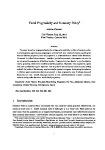
2 (6) ³ ´2 2 = 2 + 2 − 2 (7) £ ¤ where = + (1 − ) The optimal policy space is a 3 − and is a + proper subset of R3 . Figure 1 shows a subset of the hyperplanes in o . The set o is composed by an infinite number of the hyperplanes in the figure, each indexed by a value for 2 since the range of observable outcomes for 2 is bounded from below, but not from above. In this instance, the model implies that only a limited subset of macroeconomic outcomes is optimal, though the set o encompasses a very large range of outcomes. To obtain much tighter restrictions on o we compute the mapping (; o) 9
for the set of endogenous variables ( )5 Conditional on the optimal policy (4), define: ⎤ ⎡ ⎤ 2 2 2 2 ⎥ ⎢ ⎥ ⎢ 1 2 2 (; o) ≡ ⎣ 2 ⎦ = ⎣ 2 2 2 + 2 (1− ⎦ − 2 ) (1− ) 2 ( )2 2 + 2 − 2 ⎡
where = [ 2 2 ]0 The set o for this model is a 3 − , as can be checked by computing [g ]. The optimal policy space is shown in figure + 2 Contrary to the earlier case, the set o ⊆ R3 for ( ) includes a set of outcomes for 2 bounded from above and below for any ( 2 2 ). The intuition for the result is straightforward. Even if conditional on the optimal policy demand e they affect and As a consequence, for shocks e do not affect and 2 given optimal outcomes where 2 is larger imply that 2 is larger too. As for cost-push shocks , they increase the volatility of all three variables. + The set o is not of measure zero. Optimal outcomes in the R3 space do not align on a two-dimension hyperplane because for different combinations ( 2 2 ) there may exist more than one outcome for 2 corresponding to the same outcome ( 2 2 ) + Note that parameterizations where o is of measure zero in R3 do exist. If = = 0, using the definitions for and we obtain: ⎤ ⎡ ⎤ 2 (2 + )−2 2 2 ⎥ ⎢ ⎥ ⎢ (; o) ≡ ⎣ 2 ⎦ = ⎣ 2 (2 + )−2 2 + 12 2 − 2 2+ ⎦ 2 ()2 (2 + )−2 2 + 2 − 2 2+ ⎡
(8)
Eq. (8) shows that 2 = 12 2 for any value of and Therefore the Jacobian of (; o) has two proportional columns for any . Since [g ] = 2 the i h 1 Since = ∗ + e it holds that = − (1− e + e where the technology shock is an ) AR(1) stochastic processes with autocorrelation parameter In deriving the equation for we also assume the government spending shock is an AR(1) stochastic process with autocorrelation parameter = and steady state government spending is zero. 5
10
optimal policy space cannot be a 3 − . The image can be parameterized by the function : ⊆ R2 → R3 : ⎤ 1 ⎥ ⎢ () ≡ ⎣ 2 ⎦ 2 2 ⎡
where 1 = 2 (2 + )−2 2 and 2 = 2 (2 + )−2 2 + 12 2 − 2 2+ In this case, o is a 2 − in R3 implying any outcome is suboptimal almost surely. In general, by finding the appropriate combination of endogenous variables, it may be possible to obtain an optimal policy space conditional on a model (; ) that includes only a bounded set of outcomes for at least one variable. While we illustrated the methodology with an example where we can derive analytically the mapping (; ) the set o can be obtained for any DSGE model, and for an appropriately chosen vector of endogenous variables using numerical methods. 6 The set o can be used to assess the restrictions the optimal policy implies for observable economic volatility. This methodology can be readily extended beyond the case of optimal policy rules. It can in fact be employed to define the volatility space for given rule for monetary policy, including any functional form for a policy rule depending on endogenous variables. The volatility space will then define the set of outcomes related to a given Taylor rule, assuming the policymaker never deviates from the interest rate prescribed by the rule, and for any value of the Taylor-rule parametervector. The volatility space for a Taylor rule functional form can be easily compared with the optimal volatility space, in a given model. As an example, consider the optimal policy defined in eq. (4). It can be implemented by the instrument rule:
6
= +1 + e
(9)
o can be built using either numerical simulation or, in the case of linear equilibrium law of motions, the endogenous variables’ volatility implied by the reduced-form representation.
11
A suboptimal Taylor rule, could be described by the instrument rule in eq. (9) under the assumption that the coefficient summarizing the response of policy to expected inflation be different from : = +1 + e
The volatility space conditional on the Taylor rule will be different from the optimal policy space. First, the vector now includes the value for the coefficient This, in itself, provides an additional degree of freedom. However, we cannot draw a general inference about the resulting implications for the size of the volatility space relative to the optimal policy space, since also the law of motion for all endogenous variables will now be dependent on The mapping between the volatility of exogenous shocks and the volatility of endogenous variables depends nonlinearly on the model parameters, therefore the added degree of flexibility in the parameterization may only lead to volatility outcomes which already belong to o . This for example is the case in our baseline model, where eq. (4) shows that e only depends on the ratio the relationship between the volatility of and and not on each of the two parameters independently.
4
United States Volatility Outcomes and Optimality of Monetary Policy
4.1
Restrictions from the New Keynesian Model and Implications for Historical United States Macroeconomic Volatility
As an illustration of our methodology, consider the optimal policy space for the variables ( ) conditional on the model in eqs. (1), (2), (3). We consider two sets of parameters and several alternatives for the implied optimal policy, depending on the choice of objective function and the definition of optimality
12
adopted. We allow for endogenous inflation persistence by setting = 05 and consider an economy with a distorted steady state, so that any shock will affect all the endogenous variables under the time-consistent optimal policy. While this is a stylized model, it is widely used in theoretical and empirical work. Since the model’s equilibrium law of motion has multiple endogenous and exogenous state variables, it is not feasible to build analytically the mapping (; ) as in section 3. The set of optimal outcomes o is instead computed numerically by solving the model over a multi-dimensional grid of the parameter’s space, and finding for each parameterization the implied volatility of the endogenous variables. In our first experiment, we examine the optimal policy space fixing the model’s deep parameters, except for the values of the shocks’ volatilities and the objective function parameter We assume that the relative weight across objectives in the policy objective function is of the deep parameters of the model, so that = [ ]0 . 7 This allows the central banker to have a different welfare definition from the social welfare, which is defined by the utility functional of the representative agent. Computationally, it relaxes the restriction linking to the deep parameters of the model. Figure 3 plots o (similar in shape to the plot in figure 2) for the time-consistent optimal policy, together with the outcome ( ) for the U.S. over the period 1984:1 - 2005:1. There is no combination of the volatility of exogenous shocks and policymaker preferences that could have generated the observed ( ) as an optimal policy outcome. We then build the function (; ) for the time-consistent optimal policy and for = [ ]0 . Unless otherwise specified, in this and all the following experiments we assume the policymaker preferences maximize the representative household’s utility, so that the value of in eq. (3) is a well-defined function of the values chosen for the deep parameters, and does not need to be included in the vector . We include in the structural parameters of the model, presented in the Appendix: is the share of firms that cannot optimally adjust the price in each period, is the fraction of last period’s aggregate inflation rate to which the share of firms indexes the price, is the firms’ demand elasticity, is the 7
Using = [ ]0 would generate the same image for (; o)
13
inverse of labor supply wage elasticity. Table 1 reports the range of variation for the model’s parameters. 8 Even allowing for a larger set we still obtain that o . ( ) ∈ Finally, our numerical results show that the outcome ( ) does not belong to o for a number of alternative objective functions. This result holds under the assumption that the policymaker adopts the timeless perspective optimal commitment policy, and under the alternative assumption that the policymaker adopts the wrong objective function assuming = 0 in eq. (3), a case considered in Walsh (2005). We also examine the optimal policy space for a time-consistent policy where the policymaker’s objective function allows for an interest rate-smoothing objective, as suggested by Woodford (2003). Including an interest rate smoothing objective may improve welfare outcomes, even if the reduction of interest rate volatility is not a social objective in itself. We define: X © ª 1 e e2+ + 2+ + ∆ ( − −1 )2 = − Ω 2 =0 ∞
and compute the optimal policy space for = [ ∆ ]0 Also in this case, the outcome ( ) does not belong to o These results can be explained by two observations. First, all the model parameterizations imply different responses of endogenous variables to exogenous shocks. But many of the resulting models are nearly observationally equivalent in terms of unconditional volatility outcomes ( ): the same outcome ( ) can be generated with alternative parameterizations by different vectors [ ]0 . Second, changes in a parameter do not necessarily add useful degrees of freedom to enlarge o . For example, in the optimal policy space 8
We verified that ( o by searching for a vector = [ ]0 such ) ∈ that ( ) is in the ±25% interval around the data point ( ) Allowing for a range of variation in ( ) lets us account for the numerical error in the approximation to (; ). The map (; ) is computed through a discrete approximation over 3,686,000 simulated data points. Admissable parameter values outside the range in table 1 result in outcomes further away from the historical observation for the US. Note that including additional parameters in does not necessarily result into ( ) ∈ o because of the nonlinearity of the mapping (; o)
14
for ( ) of the basic new Keynesian model a change in is observationally equivalent to a change in , since the relationship between e and and between e and in eqs. (6) and (7) depends on the ratio . The difficulty in finding a model within the parametric family such that the U.S. outcome belongs to the optimal policy space has three alternative interpretations. First, U.S. monetary policymaking was indeed suboptimal. After all, the building of the optimal policy space does allow for any possible parameterization in the vector [ ]0 including parameterizations that may be inconsistent with available empirical evidence, and is robust to several alternative assumptions for the optimal policy computation. Finally, the optimal policy space has by construction weak power against detecting suboptimal policies: historical outcomes may belong to o even if they are the result of period-by-period suboptimal policies. Second, the DSGE model propagation mechanism is incomplete or inaccurate. Conditional on optimal monetary policy, it puts implausible restrictions on the endogenous variables’ variances. This conclusion leads to question whether the optimal policy prescriptions derived from stylized DSGE models such as the one used are appropriate to guide real-world policymaking. Medium-scale models, such as the Smets and Wouters (2007) model, may provide more flexibility in terms of the parameterization of the functional forms describing the dynamics of the endogenous variables belonging to the optimal policy space. As the number of free parameters increases, for a given set of variables, there is the chance that the optimal policy space will span a larger subset of the variables’ volatility space. At the same time, the map (; ) depends on the equilibrium law of motion for the endogenous variables, therefore the cross-equation restrictions across a larger number of parameters may imply that the optimal policy space will span a smaller subset of the variables’ volatility space, relative to the stylized model we considered. Third, the information set of the policymaker may be different from the one available to the econometrician. This implies that the policy assessment computed with final data for the endogenous variables may erroneously conclude that policymaking was suboptimal even if the monetary authority was reacting optimally to the information available in real time. Consider for example the target rule for 15
optimal policy defined in equation (4). If the policymaker can only measure the output gap with a random observation error the targeting rule yields: = − (e + )
(10)
implying for given volatility of the output gap, the volatility of inflation increases. The targeting rule (10) though assumes that the policymaker is not aware of the observation error - for example, of future revisions for the final data on GDP, productivity or employment. Within the stylized model we consider in this section, when endogenous variables are imperfectly observed the true optimal policy is given by: |Ω } (11) { |Ω } = − {e Note that the problem of imperfect observability of the true macroeconomic aggregates - that is, the problem of conducting policy using real-time data - does not necessarily imply that the aggregate volatility of macroeconomic variables will increase. When the optimal policy is chosen according to eq. (11), it can be shown e are given by that the resulting optimal imperfect-information outcomes and
¶ µ 2 + e = 1+
;
e =
1 e
(12)
where is the perfect-information outcome, and to facilitate comparison with the perfect information case we assumed that all exogenous shocks are iid. 9 Compared to the case of perfect information, equation (12) implies that inflation volatility will increase, while output-gap volatility may increase or decrease, depending on the relative volatility of demand and cost-push shocks. However, since the optimal volatility space will change, this example shows that taking into account the information set Ω available to the policymaker can play a potentially important role when using our suggested methodology to assess policy outcomes. 9
For further discussion of the issue of policy assessment under imperfect information, see Clarida, Gali and Gertler (1999).
16
4.2
A Probabilistic Interpretation of the Inefficiency of a Volatility Outcome
The optimal policy space does not provide a measure of the distance between an inefficient volatility outcome and the set of efficient outcomes. In this section we define such a measure by evaluating how large an additional source of randomness in the model should be for an inefficient outcome to belong to the set o Note that this assessment relies on final data, rather than the real-time information set available to the policymaker. Therefore, our measure of deviation from the optimal policy outcome may in part be explained by the difference in the information set available to the econometrician and to the policymaker. Consider the largest optimal policy space built to assess the U.S. macroeconomic performance in the previous section, where we assumed = [ ]0 The monetary authority enforces the time-consistent optimal policy, and the deep parameter values are summarized in Table 1. We now assume the observable interest is described by rate = + where is a random variable with variance 2 = 100 2 The value gives the variance of the variable as a percent share of the variance of the unobservable variable which is assumed to behave according to the optimal policy. In the econometric literature is assumed to represent a measurement error. It can be interpreted as summarizing the volatility in which is not explained by the DSGE model. By adding a third source of randomness, we enlarge the set o of optimal policy outcomes, and obtain a measure of how large deviations of from the volatility implied by the optimal policy need to be to have a nonzero probability of observing the outcome ( ) conditional on the data-generating process in eqs. (1), (2), (3) and on all possible vectors = [ ]0 For each value of we compute the probability of a given bounded set around ( ) over all the outcomes () The probability is calculated for the standard deviation of a variable belonging to the 5% interval [ ] centered around the
17
observation Finally, let o ⊆ + be the optimal policy space for the variable + and o ⊆ 2 be the optimal policy space for the variables ( ) To scale the result we compute the probability of an outcome ∈ [ ] belonging to o conditional on any value within the 5% interval for ( ) belonging to o Formally, we compute Pr
(
) ¤ £ ) | ( ∈ o ) ∩ ( ≤ ≤ [( ) ∈ o ∩ ( ≤ ≤ ) ∩ ( ≤ ≤ )]
Figure 4 plots the conditional probability against the variance 2 computed as a percent share of the variance 2 Including a third source of randomness implies that the outcome ( ) can be the result of optimal policymaking, and the variable provides a simple measure of the additional randomness needed for the U.S. observation to belong to o
5
Related Literature
A growing literature investigates the data fit of micro-founded DSGE models to the data conditional on an optimal monetary policy. Most related research focused on forward and backward-looking small macroeconomic models used in the monetary policy literature. Soderstrom et al. (2002) use informal calibration to match an optimal policy new Keynesian model dynamics to U.S. data. Dennis (2004), Favero and Rovelli (2003) and Salemi (2006) estimate structural models subject to the restriction that the policy rule minimizes the policymaker loss function. Given a time series for the observables (1 ) with covariance matrix Σ the approach adopted by these authors produces estimates for the deep parameters, the policymaker preferences, and a time series for a vector of shocks with nonsingular covariance matrix such that the theoretical model can generate the historical data. This approach also implies that there will exist an estimated parameter vector, including random deviations from the optimal policy, such that the historical volatility outcome can be generated by the model. 18
Salemi (2006) shows how to use the nonsingular model estimation approach to compute a statistical test for optimal policymaking. The optimal policy imposes cross-equation restrictions on the estimated parameters, and their impact on the likelihood of the model can be exploited for testing. The optimal policy space we propose is instead built exploiting the restrictions imposed by truly optimal policymaking in a parametric family of singular models on the volatility of observable variables. Compared to the assumptions used by papers estimating a non-singular model with deviations from the optimal policy behaviour, the singularmodel approach we propose makes stronger assumptions on the behaviour of the policymaker. On the other hand, the use of the optimal policy space as a diagnostic tool for the efficiency of macroeconomic outcomes relaxes the demand on the data fit since policies that are period-by-period suboptimal may still result in volatility outcomes belonging to the optimal policy space. Clearly a three-equations model, as the one adopted in this paper, can only provide a stylized description of the economy’s behaviour. Yet small optimal policy DSGE models are estimated to gain insight into the preferences of the policymaker, and are often relied upon by economists to illustrate and generate policy prescriptions and guidelines. Computing the optimal policy space for such models provides important insights into the restrictions on the data that the models imply.
6
Conclusions
This paper studied the restrictions implied by optimal policy DSGE models for the volatility of observable endogenous variables. Our approach relies on the restrictions imposed by optimal policymaking on the variance of the endogenous variables in singular models. To generate a non-trivial set for the volatility of observable variables - which we label the optimal policy space - we introduce variation in the behavioral parameters when building the set of outcomes consistent with the model. We show that a DSGE model can be associated with a well-defined subset of all the possible volatility outcomes, which is not of measure zero. This is the result of the nonlinearity of the mapping be19
tween a DSGE model parameter space and the implied volatility of the endogenous variables. Nonsingular models, which assume random perturbations to optimal policymaking, imply no observable outcome has zero probability. We illustrated our method by building the optimal policy space of a widely used new Keynesian model. Conditional on this model, recent U.S. monetary policymaking would have zero likelihood of being the result of optimal policymaking. Since this approach has by construction low power in discriminating optimal policy outcomes, we interpret the result as evidence that widely used optimal policy models can only be consistent with a very limited set of volatility outcomes, regardless of the parameterization adopted. In the case of a simple new Keynesian model we were able to find a closed-form solution for the mapping (; ) defining the optimal policy space, describing the volatility of endogenous variables as functions of the volatility of exogenous shocks. When a closed-form solution is available, the rank of the Jacobian matrix associated with (; ) can be examined to assess whether the optimal policy space for a given set of endogenous variables is of measure zero. We showed that when a closed-form solution is not available, numerical simulations can be performed to generate the optimal policy space. Thus this approach can be readily extended to medium-scale DSGE models.
References [1] Baxandall, P. and Liebeck, H., (1986), Vector Calculus, Oxford: Clarendon Press. [2] Benigno, P. and Woodford, M., (2005), ”Inflation Stabilization and Welfare: the Case of a Distorted Steady State”, Journal of the European Economic Association 3(6): pp. 1185-1236. [3] Bierens, H., (2007) "Econometric analysis of linearized singular dynamic stochastic general equilibrium models", Journal of Econometrics 136: pp. 595-627.
20
[4] Clarida, R., Galí, J., and M. Gertler, (1999), “The Science of Monetary Policy: A New Keynesian Perspective,” Journal of Economic Literature, 37, 4, pp. 1661-1707. [5] Conlon, L., (2001), Differentiable Manifolds, Boston: Birkhauser. [6] Dennis, R., (2004), ”Inferring Policy Objectives from Economic Outcomes”, Oxford Bulletin of Economics and Statistics 66: pp. 735-764. [7] Favero, C. and Rovelli, R., (2003), ”Macroeconomic Stability and the Preferences of the Fed: A Formal Analysis, 1961-1998”, Journal of Money, Credit and Banking 35: pp. 546-556. [8] Kwakernaak, H., (1979), "Maximum likelihood parameter estimation for linear systems with singular observations", IEEE Transactions on Automatic Control AC-24:3. [9] Lai, Hung-pin, (2008), "Maximum likelihood estimation of singular systems of equations", Economic Letters 99: pp. 51-54. [10] Salemi, M., (2006), ”Econometric Policy Evaluation and Inverse Control”, Journal of Money, Credit and Banking 38: pp. 1737-1764. [11] Soderstrom, U., Soderlind, P. and Vredin, A., (2002), ”Can a Calibrated New Keynesian Model of Monetary Policy Fit the Facts?”, Sveriges Riksbank Working Paper 140. [12] Walsh, C., (2005), ”Endogenous Objectives and the Evaluation of Targeting Rules for Monetary Policy”, Journal of Monetary Economics 52: pp. 889-911. [13] Woodford, M., (2003), "Optimal interest rate smoothing", Review of Economic Studies 70: pp. 861-886.
21
New Keynesian model parameter range for U.S. optimal policy space 0.2-0.82
0.1-0.66 0.1-1.17
4-16
Table 1: New Keynesian model parameter space used to compute optimal policy space o = (; ) for = [ ]0 Other parameters are set as in Walsh (2005). Model is described by the time-consistent solution to maximization of eq. (3) given eqs. (1), (2) and assuming the policymaker’s objective function maximizes the utility of the representative household Parameter is the share of firms that cannot optimally adjust the price in each period, is the fraction of last period’s aggregate inflation rate to which the share of firms indexes the price, is the firms’ demand elasticity, is the inverse of labor supply wage elasticity. Parameter values outside the range in table 1 result in outcomes ( ) further from the historical U.S. observation for the sample 1984:1-2005:1.
22
2
2
2
Optimal policy space for , x , i
0.7
0.6
Variance (interest rate)
0.5
0.4
0.3
0.2
0.1 lower bound for 2 i
0 0.35 0.3 0.9
0.25
0.8 0.7
0.2 0.6
0.15
0.5 0.4
0.1
0.3 0.2
0.05 0.1 0
0
Variance (inflation)
Variance (output gap)
Figure 1: Optimal policy hyperplanes belonging to the optimal policy space o for the variables ( e ) and for = [ 2 2 ]0 using the baseline new Keynesian model. Each hyperplane is indexed by a value for 2
23
2
2
2
Optimal policy space for , y , i
0.3
.25
0.2
.15
0.1
.05
0 0 1 2 3 4 5 6 7 8
0.05
0
0.1
0.15
0.2
0.25
Variance (inflation) Variance (output)
Figure 2: A subset of the optimal policy space o for the variables ( ) and for = [ 2 2 ]0 using the baseline new Keynesian model. 24
0.3
0.35
Figure 3: A subset of the optimal policy space o for the variables ( ) and for = [ ]0 using a new Keynesian model with endogenous inflation persistence and a distorted steady state. The plot shows the historical volatility outcome for the U.S. over the period 1984:1 - 2005:1. Output is detrended seasonally adjusted non-farm business sector real GDP. Inflation is seasonally adjusted CPI inflation. Interest rate is 3-month government bond. All data is sampled at quarterly intervals.
25
Probability of US outcome ( 2 , 2y , 2i ) belonging to optimal policy space
1
0.9
0.8
0.7
Likelihood
0.6
0.5
0.4
0.3
0.2
0.1
0
0
10
20
30 40 50 60 70 80 Interest rate measurement error variance - percent share
90
Figure i £4: Probability of the ¤outcome h £ ¤ { ∈ (±25% × ) ∩ ∈ (±25% × ) ∩ ∈ (±25% × ) } belonging to the optimal policy space o conditional on the outcome ¤ £ ¤ £ { ∈ (±25% × ) ∩ ∈ (±25% × ) } belonging to the optimal policy space o Horizontal axis measures variance of the measurement error for as a percent share of the variance for the optimal observed interest rate 2 . interest rate given by 2 = 100 26
100
27
7 7.1
Appendix The Optimal Policy Space for a Singular Model: the Case of a Linear Mapping ()
This section shows that for a singular model, as in the case of a parameterized linear optimal policy DSGE model, the mapping () is linear. Assume (; o) is a linear map and is equal to: (; o) = C
(13)
where is an × 1 vector and C is an × matrix. For an unrestricted vector two outcomes are possible. When the matrix C is of rank its columns span the space R Then o = R and necessarily o = p for any policy p such that (C) = When C is of rank its columns span the subspace R and o is a -dimension hyperplane. For a linear model and including only the entries for the exogenous shocks’ covariance matrix the map (; o) can be written as in eq. (13). Let the model associated with (; o) be described by the stationary law of motion = A where is an × 1 vector of endogenous variables with covariance matrix Σ and is an × 1 vector of exogenous shocks with covariance matrix Σ For ≡ (Σ ) we can write (; o) = T (A ⊗ A) (Σ )
(14)
where T is an × matrix with unitary value at entry [ ( − 1) + ]=1 and zero otherwise, so that (; o) is equal to the diagonal of Σ . If A is of rank the linear map (Σ ) = (A ⊗ A) (Σ ) spans the space defined by the vectorization of × positive semi-definite symmetric matrices, and the matrix T (A ⊗ A) is of rank Because Σ is a positive semi-definite symmetric matrix, (; o) does not + span R It will though span R since (; o) is just the main diagonal of Σ + and any vector ∈ is the main diagonal of at least one positive semi-definite 28
matrix. If A is of rank also T (A ⊗ A) is of rank This is the case of a singular model, where o is a -dimension hyperplane in R Therefore, conditional on the model A either vectors [21 22 2 ]0 belong to the optimal policy + space (and o is an improper subset of R ) if = , or any vector [21 22 2 ]0 almost surely does not belong to the optimal policy space if
7.2
Solution of the Benigno and Woodford (2005) Model
Consider the New Keynesian model for inflation output gap , interest rate as described in Walsh (2005) and Benigno and Woodford (2005): 1 = − ( − +1 − ) + (+1 ) e ( +1 − ) − −1 = +
(15) (16)
= −
where is the Wicksellian real rate of interest, is output, is the level of output that would obtain in the flexible-price equilibrium, is the coefficient of relative risk aversion for the representative household divided by the consumption e is the household’s discount rate. It is assumed that a constant share of output, share of firms can adjust the price in each period, while the remaining share indexes the price to a fraction of last period’s aggregate inflation rate. When prices can optimally adjust in every period the rational expectation equilibrium solution for
29
and does not depend on : = 1 + 2 + 3 = 4 (+1 − ) + 5 (+1 − )
+ (1 + ) = + [ (1 − )] = + =
1 = 2 3 4
5 = (1 − ) = (1 + ) − 1 The variable is defined as exogenous government consumption (in log-deviations from the steady state), is an exogenous productivity shock, is an exogenous income tax shock. The parameter is the elasticity of firm output with respect to labor input, is the inverse of the wage elasticity of labor supply, is the inverse of the elasticity of firm marginal cost with respect to output, is the steady state tax rate, is the consumption steady state share of output, is the coefficient of relative risk aversion for the representative household divided by The elasticity of inflation with respect to is given by: =
e (1 − )(1 − ) ( + ) (1 + )
In the absence of transfers to correct the steady state distortions arising from taxes and imperfect competition, or in the case 6= 0 the efficient level of output ∗ is
30
different from and is given by: ∗ = 1 + 2 + 3 + + Φ(1 − ) Φ = ( + ) = (1 − )
1 = 2 3
= ( + ) + Φ(1 − ) − Φ = 1−
Φ(−1 − 1) ( + )
−1 (1 − )
where is the firms’ demand elasticity. The second order approximation to the utility of the household can be written as:
X © ª 1 e e = − Ω 2+ + (+ − +−1 )2 2 =0 ∞
(17)
e = ( − ∗ )
where e is the welfare-relevant output gap is equal to the household’s welfare for = ∗ where ∗ = 1 The model in (15), (16) can be expressed in terms of the endogenous variables appearing in the objective function (17): 1 +1 ) e = − ( − +1 − e ) + (e e ( +1 − ) + − −1 = e +
∗ e = 4 (+1 − ∗ ) + 5 (+1 − )
= ∗ −
31
(18) (19)
The variable is a linear combination of all the exogenous shocks. The variable Φ is a measure of the steady state distortions in the economy. If appropriate transfers ensure, as is often assumed, that the steady state is efficient, then Φ = 0. Benigno and Woodford (2005) show that in this case 1 = 1 2 = 0 and = 3 Assume = 0 Then the problem faced by the optimal policymaker can be written as: ∞ X © 2 ª 1 e e + + 2+ (20) − Ω 2 =0 1 +1 ) e = − ( − +1 − e ) + (e e +1 + + = e = 3
e = 4
∙
(21) (22) ¸
(23)
(+1 − ) + (1 + )(+1 − ) + 5 (+1 − ) (24) +
In this model movements in or can be interpreted as ’demand shocks’ since they affect e but not therefore do not affect the trade-off between the stabilization objectives and can be perfectly offset by the policymaker. The variable takes the interpretation of a ’cost push’ shock, and depends only on movements in . Assuming, as in eq. (??), that = 1 = −1 + = −1 + ∼ , = it holds: ∗ e = 4 (+1 − ∗ ) 1 ∗ = − e (1 − )
Eq. (25) holds also for 1 and = 0 ∀ or for 1 and = 1
32
(25)
The optimal time-consistent policy is given by the FOC: e − −1 = − (1 + )
The timeless perspective optimal commitment policy is given by the FOC: − −1
³ ´ ( − −1 ) = −
Baseline parameterization The parameterization follows Walsh (2005) unless otherwise stated in the main text. = 066 = 05 e = 099
= 016 = 15 = 788 = 08 = 049 = 02 = 095 = 095 = 095
33