On Finding the Point Where There Is No Return: Turning Point Mining on Game Data (Supplementary Material) Wei Gong∗

Ee-Peng Lim∗

Feida Zhu∗

Palakorn Achananuparp∗

David Lo∗

1

Proof of Apriori Property for Frequent ordered pattern satisfying Apriori property. Patterns Apriori Property. If a pattern is frequent in a game 2 Proof of Property 1 dataset D, then all its sub-patterns are also frequent in D. Proof. If a pattern has sub-patterns, then the pattern is either a conjunctive pattern or an ordered pattern. We therefore prove that both types of pattern satisfy Apriori property. Let p0c be a conjunctive pattern, and a game S in D satisfies p0c . Suppose there exists pc which is a sub-pattern of p0c , such that S does not satisfy pc . By the definition of conjunctive pattern, since S does not satisfy pc , then S does not satisfy at least one simple pattern, e.g., ek in pc . Because pc v p0c , ek is also in p0c , then S does not satisfy p0c which implies a contradiction. Therefore, the games in D satisfying p0c will also satisfy all the sub-patterns of p0c , which implies frequent conjunctive pattern satisfying Apriori property. 0c 0c Let p0o = p0c 1 ≺ p2 ≺ . . . ≺ pm be an ordered pattern, and a game S in D satisfies p0o . Then there 0 }, exists at least one instance of p0o in S: {I10 , I20 , . . . , Im 0 0c 0c 0 I1 ∈ I(p1 , S), . . . , Im ∈ I(pm , S), such that ∀t1 ∈ 0 I10 , . . . , ∀tm ∈ Im , t1 < t2 < . . . < tm . Let po = pc1 ≺ c c p2 ≺ . . . ≺ pn is a sub-pattern of p0o , then there exists integers 1 ≤ k1 < k2 < . . . < kn ≤ m such that pc1 v c 0c c 0c p0c k1 , p2 v pk2 , . . . , pn v pkn . Since we already proved that conjunctive patterns satisfy Apriori property, there exists I1 , I2 , . . . , In , I1 ∈ I(pc1 , Si ), . . . , In ∈ I(pcn , Si ), such that I1 ⊆ Ik0 1 , . . . , In ⊆ Ik0 n . Since 1 ≤ k1 < 0 k2 < . . . < kn ≤ m, and ∀t1 ∈ I10 , . . . , ∀tm ∈ Im , t1 < t2 < . . . < tm , we get that ∀t1 ∈ I1 , . . . , ∀tn ∈ In , t1 < t2 < . . . < tn . Hence, there exists an instance of po in S {I1 , I2 , . . . , In }, I1 ∈ I(pc1 , S), . . . , In ∈ I(pcn , S), such that ∀t1 ∈ I1 , . . . , ∀tn ∈ In , t1 < t2 < . . . < tn . Therefore, S satisfies po . Thus, we also have frequent

Property 1. Let p = pc1 ≺ . . . ≺ pcm be a frequent pattern in a game dataset D. If pcm+1 is frequent in the p-projected DB, then p ≺ pcm+1 is frequent. Proof. Since pcm+1 is frequent in p-projected DB, then we know that there exists no less than min_sup games in p-projected DB that pcm+1 occurs after p. Therefore, p ≺ pcm+1 is frequent. 3

Proof of Property 2

Property 2. Let pc1 ≺ . . . ≺ pcm be a frequent pattern in D. If a simple pattern ei is frequent in pc1 ≺ . . . ≺ pcm projected DB, then pc1 ≺ . . . ≺ pcm ≺ ei is also frequent in D. If ej is frequent in pc1 ≺ . . . ≺ pcm -projected tagged DB, where ej 6∈ pcm , then pc1 ≺ . . . ≺ pcm ∧ ej is also frequent in D. Proof. The first part of the property is Property 1. Here we prove the second part. Any projected tagged game in pc1 ≺ . . . ≺ pcm -projected tagged DB satisfies pcm , and ej is frequent in pc1 ≺ . . . ≺ pcm -projected tagged DB where ej 6∈ pcm , so pcm ∧ ej is frequent in pc1 ≺ . . . ≺ pcm -projected tagged DB. As pc1 ≺ . . . ≺ pcm−1 projected DB is a superset of pc1 . . . ≺ pcm -projected tagged DB, pcm ∧ ej is also frequent in pc1 . . . ≺ pcm−1 projected DB. According to Property 1, we can conclude that pc1 ≺ . . . ≺ pcm−1 ≺ pcm ∧ ej is frequent in D. 4

Tic-Tac-Toe (TTT) Game Generation

To learn TPRs from TTT games, we first generate game datasets synthetically by making use of a well-known heuristic strategies of the game [1] to simulate players playing TTT. The heuristics consists of a set of eight strategies, namely win, block, fork, blocking fork, play center, play opposite corner, play empty corner, and play empty side. ∗ School of Information System, Singapore ManageA game dataset requires two different outcomes. ment University. (email: [email protected], This means players X and O cannot both always follow [email protected], [email protected], [email protected], the heuristics. In this case, the games will always be [email protected])

drawn. We therefore create a probabilistic heuristic algorithm called Strategy to control the abilities of players, such that we can simulate players with various playing skills. Strategy assumes that every player must follow the win and block strategies as we do not want the player to lose too easily. When the above two strategies are not applicable, the player uses a parameter β ∈ [0, 1] to control the probability that she follows the remaining strategies. When β = 1, Strategy works the same as the original heuristics and will never lose the game. With Strategy, we now can generate a set of games with both XW and XN W outcomes involving players of abilities controlled by their β values. TPRs with outcome XW then can be mined from the datasets. Note that TPRs with outcome OW (O wins) can also be mined from the same dataset, we only need to change the labels of the outcomes to OW and ON W . 5

Applying TPRs to Play TTT Games

In this section, we show some interesting findings when we apply TPRs to play TTT games. The main idea here is to recommend game moves that lead to TPR patterns, so as to increase the chances of winning given that TPRs are strong and offer irreversible outcome property. 5.1 Algorithms for Applying TPRs in TTT We propose two algorithms that employ TPRs to guide game playing. The first algorithm, TPR+RANDOM (TR), uses TPRs only. The second algorithm, called TPR+ STRATEGY (TS), uses both TPRs and Strategy. Both algorithms call a common function TPRRec that incorporates TPRs in recommending the next move. TPRRec is shown in Algorithm 1. Algorithm 1 TPRRec 1: input: player u, set of TPRs for u to win T P RSetu , current game sequence CG, probability that opponent is assumed to follow in Strategy βa 2: output: recommended move mover 3: procedure TPRRec(u, T P RSetu , CG, βa ) 4: mover = null, confr = 0 5: M oveSet = available next moves in CG 6: foreach move ∈ M oveSet 7: CG0 = game sequence after player u makes the move 8: foreach rule R ∈ T P RSetu 9: if MatchRule(CG0 , R, βa ) is TRUE 10: if conf (R) > confr 11: conf r = conf (R), mover = move 12: return mover 13: end procedure

some TPR later. MatchRule in line 9, simulates both players’ moves from CG0 until the game ends, and check whether the final game sequence satisfies some TPR R. We simulate players’ moves in the following way. Suppose X uses TPRs for XW , in order to reach a TPR, X chooses the moves that make the game closer to the pattern. For O, we simulate his/her moves by using an assumed parameter βa to measure how likely O follows the heuristic strategies. Note that βa is adopted to simulate the opponent’s moves, but not the actual ability of the opponent. For example, suppose CG = (X1)(O3), R is X6 ∧ O7 ≺ X5 ∧ X9 ⇒ XW , and βa = 0.8. X2, X4, X5, X6, X7, X8, and X9 are the available moves for player X. Now suppose we are checking the candidate move X6, the next game sequence is then CG0 = (X1)(O3)(X6). The residue rule, which is the part of original rule R that CG0 does not match yet, is O7 ≺ X5 ∧ X9 ⇒ XW . X wishes O to choose O7, however, since O is assumed to have 0.8 probability to follow the heuristic strategies, O may or may not choose O7. If O chooses O7, then one can check that X can reach the rule later, so MatchRule returns TRUE, meaning that X6 can lead the game to R. If O does not choose O7, MatchRule then returns FALSE. Since we may find multiple moves that can lead the game to some TPR, we choose the move whose corresponding TPR has the highest confidence (lines 10 and 11). When TPRRec generates a recommendation (i.e., mover 6= null), both TR and TS will adopt the recommended move. Otherwise, TR selects the next move randomly (Random) from the available grid entries, while TS resorts to Strategy to recommend the next move. 5.2

Experimental Results

5.2.1 Experiment Setup Our experiments are designed to answer the following questions: (a) Does TPR help to recommend better game moves? (b) Can TPR based strategies perform better than methods that guarantee non-losing? Our experiments are set up in the following way. First of all, four training datasets are obtained by using our TTT game generation method with four distinct game configurations, i.e., strong X vs. weak O, weak X vs. strong O, strong X vs. strong O, and weak X vs. weak O. Note that in our experiments, if we say a player is strong (weak), meaning that she uses 0.8 (0.3) probability to play games. Other probability settings were also tested and lead to consistent results. TPRRec is to find a move from the available moves Secondly, we learn TPRs for XW from training (lines 5 and 6) using TPRs, such that the game sequence datasets. TPRs are used to play for X using TPRafter making the selected move (CG0 in line 7) can reach

Strategy_0.8 TR_LS TR_LW TS_LS TS_LW

1000 500 0 X_wins

3000

Number of games

Number of games

1500

Strategy_0.8 TR_LS TR_LW TS_LS TS_LW

2000 1000 0

O_wins

X_wins

(a) Play with strong O

(b) Play with weak O

1000 500 0 X_wins

3000

Number of games

Number of games

Strategy_0.3 TR_LS TR_LW TS_LS TS_LW

Strategy_0.3 TR_LS TR_LW TS_LS TS_LW

2000 1000 0

O_wins

X_wins

(a) Play with strong O

O_wins

(b) Play with weak O

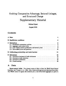
Figure 2: Performance when X is weak. Strategy_1 Minimax TR TS

1000 500 0 X_wins

O_wins

(a) Play with strong O

3000

Number of games

Number of games

1500

Strategy_1 Minimax TR TS

2000 1000 0 X_wins

XW 5381 1245 1765 3218

XN W 4619 8755 8235 6782

# of TPRs 203 20 43 102

O_wins

Figure 1: Performance when X is strong. 1500

Table 1: Training Data Distribution. Player Abilities X strong, O weak X weak, O strong X strong, O strong X weak, O weak

O_wins

(b) Play with weak O

Figure 3: Performance of different approaches. based methods TR and TS. We set min_sup as 20 games, min_conf as 1, and βa , the ability of O assumed by X to be neutral or 0.5. Thirdly, we compare our methods with Strategy playing with the same O whose abilities are controlled by Strategy with probability 0.8 (strong) or 0.3 (weak). Fourthly, the abilities of X in TS and Strategy are set consistently as in training dataset, e.g. if X is strong in training dataset, then X is also strong in testing. Moreover, we also compare our methods to the Strategy with β = 1. Other than Strategy, we also compare TR and TS with Minimax, which is a well known algorithm for games including TTT. We set Minimax to search the entire game tree. In order to evaluate the performance of the different game strategies, we count the number of games that X wins, O wins (or X loses) and draws in the test dataset. An approach is deemed better than others if it gets more wins for X and fewer for O. In our experiments, each training dataset contains 10,000 games, and each test dataset contains 3,000 games.

5.2.2 Evaluation Results Effectiveness of TPR game strategies. Table 1 shows the game outcome distributions and the number of TPRs can be mined for the different training datasets with min_sup = 20 and min_conf = 1. In Figures 1 and 2, we show the results of TPR-based methods using TPRs learnt from both strong (LS) and weak (LW) opponents. Hence, we have TR_LS, TR_LW, TS_LS, and TS_LW in these figures. The results show that under different configurations, our approaches (TR and TS) always get much more wins for X and fewer wins for O than Strategy. Hence, our approaches outperform Strategy significantly. What is more interesting is the difference between our proposed approaches TR and TS. We expect TS to outperform TR when X is strong (X wins more and also loses fewer), and the other way if X is weak. However, the results tell a different story. Figure 1 shows that when X is strong, TR leads to more wins as well as more losses than TS, which indicates that when using TPRs fails to recommend the next move, a random move is more risky than fairly strong heuristic strategies, giving a higher chance for both winning and losing. This is because while heuristic strategies, if fully followed, would prevent losing, they do not guarantee winning, which means that heuristic strategies may lead to a draw even if a player actually has a chance to win. On the other hand, a random move, albeit more risky, enjoys a greater chance to win. Hence the result in Figure 1 is reasonable. In contrast, when X is weak, as Figure 2 shows, the comparison result between TR and TS is not consistent. This is because both random moves and heuristic strategies with a low intelligence (0.3) try to take risks to win, giving ambiguous results accordingly. As Figures 1 and 2 show, in all cases regardless of the two players’ intelligence, TPRs learnt from weak players always help TR and TS (i.e., TR_LW, TS_LW) to outperform those from strong ones (i.e., TR_LS, TS_LS). The results are again different from our expectations. We expected that in order to play with strong O, we should also learn from strong O, and to play with weak O, we should learn from weak O. From our results, we can conclude that the more diverse counter play leads to better TPRs since a weak opponent plays more diverse moves because of the higher randomness.

Comparison with Strategy and Minimax. In References Figure 3, we show the performance of our methods compared with two very competitive methods, Strat[1] K. Crowley and R. S. Siegler. Flexible Strategy Use egy with β = 1 (Strategy_1) and Minimax [2] which in Young Children’s Tic-Tac-Toe. Cognitive Science, searches the entire game tree. In this experiment, both 17(4), 1993. our methods TR and TS use TPRs learnt from weak [2] S. J. Russell and P. Norvig. Artificial Intelligence: A X and weak O, which obtain the best performance as Modern Approach (2nd Edition). Pearson Education, shown in Figures 1 and 2. While TR and TS, are ob2003. served to suffer from some losses, they can achieve many more wins than Strategy and Minimax.