JOURNAL OF LATEX CLASS FILES, VOL. 1, NO. 11, NOVEMBER 2002
1
Subspace Constrained Gaussian Mixture Models for Speech Recognition Scott Axelrod, Member, IEEE, Vaibhava Goel, Member, IEEE, Ramesh A. Gopinath, Senior Member, IEEE, Peder A. Olsen, Member, IEEE, and Karthik Visweswariah, Member, IEEE
Abstract— A standard approach to automatic speech recognition uses Hidden Markov Models whose state dependent distributions are Gaussian mixture models. Each Gaussian can be viewed as an exponential model whose features are linear and quadratic monomials in the acoustic vector. We consider here models in which the weight vectors of these exponential models are constrained to lie in an affine subspace shared by all the Gaussians. This class of models includes Gaussian models with linear constraints placed on the precision (inverse covariance) matrices (such as diagonal covariance, MLLT, or EMLLT) as well as the LDA/HLDA models used for feature selection which tie the part of the Gaussians in the directions not used for discrimination. In this paper we present algorithms for training these models using a maximum likelihood criterion. We present experiments on both small vocabulary, resource constrained, grammar based tasks as well as large vocabulary, unconstrained resource tasks to explore the rather large parameter space of models that fit within our framework. In particular, we demonstrate significant improvements can be obtained in both word error rate and computational complexity.
I. I NTRODUCTION TATE of the art automatic speech recognition systems typically use continuous parameter Hidden Markov Models (HMMs) for acoustic modeling. One of the ingredients of the HMM models is a probability distribution ������ � � for the acoustic vector ��
�� at a particular time, conditioned on an HMM state � . Typically, the distribution for each state is taken to be a Gaussian mixture model. When selecting these Gaussian mixture models, the goal is to invest the modeling power and computational time required for decoding wisely. A general approach to achieving this goal is to determine a family of Gaussian models to which each component of the GMM for each state is constrained to belong. In this work we describe a framework for constraining parameters that naturally generalizes many previous successful approaches and provides the system designer flexibility in choosing an optimal compromise between speech recognition performance and computational complexity. The simplest approach to constraining the Gaussians of a model is to require all of the covariance matrices to be diagonal. Diagonal models have traditionally been used because they are simpler and much less computationally expensive than unconstrained “full covariance” models having an equal number of Gaussians. However, since the diagonal Gaussians have weaker modeling power, it has become commonplace to consider systems with very large numbers of diagonal
S
�
IBM T.J. Watson Research Center, Yorktown Height, NY 10598 axelrod,vgoel, rameshg, pederao, kv1 @us.ibm.com
�
Gaussians. This then leads back to the same problems that occurred for full covariance models – computational cost and potential overtraining due to large numbers of parameters. Approaches such as Factor Analysis [1] and Probabilistic Principal Component Analysis [2] generalize diagonal models by adding a set of rank-one terms to a diagonal covariance model. They have been applied to speech recognition with moderate success [3]–[5]. However, these direct covariance modeling techniques suffer from computational complexity problems. One approach that yields significant improvements in accuracy over simple diagonal modeling at minimal computation cost is the Maximum Likelihood Linear Transformation (MLLT) technique [6] where one still uses diagonal Gaussians, but chooses the basis in which the Gaussians are diagonal to be the columns of a linear transform which maximizes likelihood on the training data. One generalization of MLLT models are the “semi-tied full covariance models” of [7] in which the Gaussians are clustered and each cluster has its own basis in which all of its Gaussian are diagonal. Another class of models generalizing the MLLT models are the Extended Maximum Likelihood Linear Transformation (EMLLT) models [8], [9]. These models constrain the precision (a.k.a inverse covariance) matrices to be in a subspace of the space of symmetric matrices spanned by � ( ��� � ) rank one matrices, so that they may be written as follows:
��������� � � �"# ! �$ ) $ ),+$�* (1) $&% ( � ' ) The � -dimensional vectors . $0/ are the$ “tied” parameters � / are “untied” pashared by all the Gaussians and the . ' rameters specific to the individual Gaussians. The EMLLT models provide a class of models that smoothly interpolate between the MLLT models (which is the special case when � � � ) and full covariance models (where � equals the full dimension � � �2143 �6587 ). Experiments in [8], [9] showed that EMLLT models with ��9 � have lower error rate than equally computationally expensive semi-tied full covariance models with varying numbers of Gaussians and cluster centers. The MLLT technique is often used in conjunction with Fisher-Rao Linear Discriminant Analysis (LDA) technique [10]–[12] for feature selection. In this technique, one starts with an “unprojected” acoustic data vector � with some large number � of components. (Such a vector at a given time : is typically obtained by concatenating transforms of the logspectral coefficients of the waveforms for times near : .) One
JOURNAL OF LATEX CLASS FILES, VOL. 1, NO. 11, NOVEMBER 2002
2
then obtains acoustic vectors � � in some lower dimension � � by a linear projection of � by some � � � matrix � . The original formulation of LDA is motivated by an attempt to choose � � to consist of features that are most likely to have power to discriminate between states. Subsequently, Campbell [13] showed that the the projection matrix � may be calculated by maximizing the likelihood of a collection of Gaussian distributions which are tied in directions complementary to � � and which all have equal covariance matrices. The Heteroscedastic Linear Discriminant Analysis (HLDA) models of [14], [15] generalize Campbell’s models for LDA by allowing the covariance matrices in the � � directions to be Gaussian dependent. In this paper we consider state dependent distributions which are Gaussian mixture models that have the constraint that, when written as exponential models, the weight vectors are constrained to lie in an affine subspace shared by all Gaussians in the system. The precise definition of these subspace constrained Gaussian mixture models (SCGMMs) appears in section II. By imposing various conditions on the form of the constraining subspace, both the EMLLT and HLDA models arise as special cases. In section III, we summarize the computational cost for these and other special cases, including, in order of increasing generality: “affine EMLLT” models which are like EMLLT models but allow for a constant matrix (i.e. affine basepoint) to be added to the form (1) of the precision matrix; precision constrained Gaussian mixture (PCGMM) models, where the means are allowed to be arbitrary, but the precision matrices of all the Gaussians are tied to belong to the same affine subspace (of the space of symmetric matrices); and SPAM models, where separate affine subspace constraints are placed on the precisions and means (or, more precisely, on the linear weights). In each case, the computational cost for the large number of Gaussians typical in modern systems is dominated by the number of Gaussians times the dimension of the subspace to which the exponential model weights are constrained. By varying the subspace dimension, the developer is free to choose their preferred tradeoff between computational cost and modeling power. This property is one of the advantages of constraining the exponential model weights rather than the means or covariances directly. In section IV of this paper (with some additional detail in appendix II), we provide algorithms for training the parameters of models of the types discussed above using the maximum likelihood criterion. Although this training determines the continuous model parameters, it still leave many discrete choices undetermined, including: which type of model to use, what subspace dimensions to use, and how many Gaussian should be contained in the GMM for each state. These choices provides the developer a rather rich landscape of models within which to find a model that provides a preferred tradeoff between computational complexity and recognition performance. The experimental results of sections V and VI explore the landscape of possible models. The results show that one can indeed obtain an improved complexity/performance curve as each generalization is introduced. Many of the theoretical and experimental results in this
�
�
�
paper have appeared in a series of papers [16]–[20] which this paper both summarizes and extends. We have tried to make this paper as self contained as possible, although we make a few references to the previous papers for technical points. The SPAM models were first mentioned in [16], although that paper focused on the special case of precision constrained GMMs. That paper showed that the precision constrained models obtained good improvements over MLLT and EMLLT models with equal per Gaussian computational cost. Subsequent work [21] also obtained significant gains with precision constrained GMMs (although the subspace basis in [21] was required to consist of positive definite basis matrices and the experiments there did not compare to the gains obtainable with ordinary MLLT). In [20], [22], precision constrained Gaussian mixture models with speaker adaptive training were applied to large vocabulary conversational speech recognition. The precision constrained models in the experiments of [16], [20], [22] used the “modified Frobenius” basis (which approximates the ML basis and is described in section IVC) for the tied parameters and trained the untied parameters using the EM algorithm with the E-step implemented using a quasi-newton search strategy with efficient line searches. The generalization of this to the algorithm described in section IV for efficient full ML training of all parameters of a precision constrained model, although implicit in [16], was first implemented in [17]. Reference [17] also introduced affine EMLLT models and hybrid models (see section III), as well as efficient methods for training all of them. For general SPAM models, reference [18] gave efficient algorithms for finding an untied basis which approximately maximizes likelihood and for full ML training of the untied parameters given a tied basis. That paper also gave the first comparison between SPAM and LDA as techniques for dimensional reduction. Full ML training of general subspace constrained Gaussian mixture models was described in [19]. Discriminative training of these models was described in [23] and will be presented in a more systematic and rigorous manner in future work [24]. II. T HE M ODEL We consider speech recognition systems consisting of the following components: a frontend which processes a raw input acoustic waveform into a time series of acoustic feature � �� � � --- � � + , where � is a vector in �� vectors called the acoustic data vector at time frame : ; a language � model which provides a prior probability distribution � � � � � � that the --over possible word sequence user may utter; an acoustic model which gives a conditional � probability distribution � � � for the acoustic data given the word sequence; and a search strategy that finds the word sequence that (approximately) maximizes the joint � � ��� � � � � � � . likelihood � An HMM based acoustic model provides a set of states , a �� � � over possible state sequences probability � � � � distribution � � - - - + produced by a word sequence ; and probability density functions ����� � � associated with a state �
an acoustic vector � � . The state sequence � and � � � for an HMM has a particular form allowing model
�� �� � �
�
�
�
� �
� �
� ��
�
�
��
�
� � � � ��
�
�
JOURNAL OF LATEX CLASS FILES, VOL. 1, NO. 11, NOVEMBER 2002
3
efficient calculation, but everything we say in this paper applies with an arbitrary state sequence model. The conditional � distribution � � � � is written as a sum over hidden state � � � - - - � + � that may be associated with the sequences word sequence :
� � � �
� � � � � � � � � �*� �
#
� � � �*� � ��� � � �
+ �
�
�%
� We take the distributions ������ � � mixture model
#
� ��� � � �
� � � �� � � -
(3)
�
for each
to be a Gaussian
��� ������� � � � � �
������� ��
(2)
�
(4)
�
�
� ����� � � � ��������� �
��!
�#"
�
� ��!
�%$
�'&
)(+*-,/.��%$
�0&
�
�
(5)
in the form of an exponential model (as described in Appendix I). To do so, we first write the Gaussian as "
������� � � � �
�
where
7:9 � �
�
� � 8
�
� �
� 8
� $�(+1#$�2#34(�$52#6 � 147 34
� ��!
�
(6)
��� �
(7)
� ;
7
�=< >@?
�� �
1 < >@? A
�����
�
+ �2� � 8
;
8
-
(8) (9)
The inverse covariance matrix is called the precision matrix 8 and we will refer to simply as the linear weights. Next we define the feature vector B � � � and weight vector C , which are both column vectors of size � � � 1ED �6587 : B
� � � �GF
3 5 7IH
;
�
��J
��� � + �
C K
�LF
H �5J
�
��J
�� �
8
��
K
-
(10)
Here, for any � � symmetric matrix , H � *� is a column vector whose entries are the � � � 1 3 �6587 upper triangular elements of written in some fixed order, with the off diagonal elements multiplied by M 7 . This map is defined so �5J + �5J as to preserve inner product, i.e. so that H � � � H � � + � for any symmetric matrices � and . For equals N�O � � convenience, may also write column vectors as pairs, e.g. 8 � � �PH �5J � � � we C . Now we may write (6) in standard exponential model format: "SR
�
�� � �
�
��
��
�� �
�
�
� ���Q� � � �
(�T@�%$� P2#6 � 147 34
�
��
�
-
(11)
We will interchangeably use 8 � and C as is convenient. � � For example, the quantity 9 � above is a special case of the general definition of 9 � C � given in appendix I.
�
8
# � � ��� � � ������� �U � ������� � � � � � � �
�
����� � �
�
� ��� � �
"VR W
( T@�%$� P2#6 �
(12) R W
(13)
with the constraint that the C belong to a common X � 2#\Qsubspace
dimensional affine of the space of all parameters. ! Letting Y[Z � � be a basepoint of the affine space and ] be a matrix of size � � � 1^D �6587 X whose columns form a basis of the subspace, we may write:
�
���
C
where � � � � is the set of Gaussian associated to state � , � � �� � is the prior for Gaussian� � , and � ����� � � is a Gaussian distribution with mean � and covariance . For all the model types considered in this paper, the parameters for the Gaussians are required to obey a subspace constraint. To describe this, we rewrite an individual Gaussian distribution,
� � � 7
We now define a Subspace Constrained Gaussian Mixture Model (SCGMM) to be a state model
]
1
Y Z
'
� -
(14)
Note that the distribution (13) with the constraint (14) may be regarded as an exponential distribution with X 1 3 dimensional features B@_ � � , B _
�� �
�
�
`
Y Z
]ba
+
�� � -
B
(15)
From this point of view, the choice of constraining subspace may be viewed as a choice of exponential model features. III. Z OOLOGY
OF
M ODELS AND
THEIR
C OMPLEXITIES
In this section we give an overview of various special cases of the general Subspace Constrained Gaussian Mixture Models (SCGMMs) which were defined in the previous section. All the special cases arise by placing restrictions on the form of the constraining subspace. For each model type, the parameters are divided into the tied parameters, which define the subspace, and the untied parameters which specify both the point in the subspace and the prior probability for each Gaussian. Similarly, the cost of evaluating all of the Gaussians for a given input vector � is divided into two parts: the cost of precomputing the features Bc_ � � , which is the number of tied parameters (up to a constant and a factor depending on precisely how we define “computation time”); and a “per Gaussian” cost that gets multiplied by the number of Gaussians. The per Gaussian cost is the time required to calculate
�
`
3 '
�+
a
BS_
��� �
�
+
Y Z B
��� � 1
'
�+ � ] +
B
��� � �
(16)
(up to a constant term coming from the cost of adding the � precomputed values of the normalizing constant 9 � C � and exponentiating). For decoding purposes, the first term (coming from the affine shift) may be dropped because it is the same for all Gaussians and is irrelevant to distinguishing between word sequences. Table I summarizes the precomputation cost (more precisely, the number of tied parameters not counting affine shift parameters), and the per Gaussian cost (the number of untied parameters per Gaussian, not counting the prior) for various models. The first two lines are just the cost for full covariance and diagonal covariance models in dimension � , denoted FC � � � and DC � � � . Notice that neither model requires any feature precomputation and the full covariance models have a much more expensive per Gaussian cost than the diagonal models. The third line in Table I gives costs for the general subspace constrained GMM model with X dimensional feature space, denoted SCGMM � � X � . The dimension X here is free
�
JOURNAL OF LATEX CLASS FILES, VOL. 1, NO. 11, NOVEMBER 2002
4
model DC ����� FC ����� SCGMM ����"$#%� SPAM �(��"$)*" +,� PCGMM ����"4)5� EMLLT �(��"$)5� Hybrid ����"4)*"$62� HLDA ����"$��9��:�0;<;<;
to vary from all the way to the full covariance value � � � 1ED � 5 7 . Models of type SPAM � � � �� � are subspace precison and mean (SPAM) models which require the precision matrices and linear weights to be in � and � dimensional affine subspaces, respectively. � is free to range from (or 3 if no affine shift term is included) to the full covariance value of � � � 143 � 5 7 while � ranges from to � . For the SPAM models, we may write:
� �
� �
�
�
� � 8
�
Z
� �
�5J F H
�� � �
8��
K
�
��J F H �
TABLE I P RECOMPUTATION AND P ER G AUSSIAN C OSTS FOR VARIOUS S PECIALIZATIONS OF SUBSPACE CONSTRAINED G AUSSIAN M IXTURE MODELS .
(17)
(18)
���
��
Z
where � � is the � � ��1�3 � 5 7 ] ��J is �H �� � $ � and � � is the � is $ . ]
A. HLDA type models
�
�
�
'
�?@A
matrix whose � ’th column matrix whose � ’th columns
Gaussian mixture models with an affine subspace constraint � � only on the precision matrices are SPAM models with Z ] and the identity matrix. These model have untied means which may as independent parameters rather than the �$ with � � be� taken 1 3 - - - � 1 � . We call these models precision ' constrained Gaussian mixture models, denoted PCGMM � � � � in the table. The affine EMLLT models EMLLT � � � � are a special case of precision constrained models in which the basis vectors $ for the precision subspace are required to be � ) ) + 3 - - - � . Ordinary rank one matrices $ $ for � EMLLT � models don’t allow for an Z (i.e. take Z ), and so require � � � (otherwise it is not possible to obtain positive definite precision matrices). MLLT models are the special case � of EMLLT models when � � . Diagonal models are just `) - --) a MLLT models with � � equal to the identity matrix. Although the precomputation cost is a small fraction of the total cost for models considered in this paper which have a large number of Gaussians, they can become a significant part of the expense if the effective number of Gaussians needed to be computed is greatly reduced (for example by the clustering method of [18] discussed in section VII). To reduce the precomputation cost while still retaining much of the performance gain that the PCGMM models have over the EMLLT models (for example), we can use the “hybrid models” Hybrid � � � 9 � , which are precision constrained models in � which the $ , � 3 - - - � are constrained to belong to a subspace spanned by 9 rank one matrices:
� �
F
�
�
� �
�
�
� �
�
� $
�
��� ��
��
�
�
#
6
�
% �
�
�
$ ) � ),�+
� �
�
3 � ---� � -
�
�
F �
� �
�
� �� +
is
�
�
�
� F
�
��
�
� �� �
K
�� �
K
-
These constraints are equivalent to the following constraint on the exponential model weights:
� 8
�
��� ��
����
where
8
�
� � � � � �6� � ��
,
�
� �� � �
�
�
� 8
+
� �
+
� � �6�
F
F
��� �
,
�
8 8
��
�
K
(21)
�� K � �
� � � � � � � ��6� � � �
(22)
, and
�
��
�
. We call this an HLDA “type” model because one can obtain various specializations depending on what additional constraints one imposes. For example, the case with no additional constraints is the “full covariance” HLDA model considered originally in [14], [15]. As example, one could require 8 �� � � � another � and obey SPAM type constraints, that the vectors
�
# ! �$ � $ 1 $&% � '
�
2 � � �B� Z 1 # �$ � $ � Z $&% � ' ! In that case, the full model for � is a SPAM model:
� � �6� �
� � �
� +
8��
�
� +
�
F F
(20)
We could define a hybrid version of a general SCGMM model similarly, although for simplicity we have not included a separate line for such a model in Table I.
�
and the Gaussians are tied along one of the subspaces:
�
� �
� � � ���GF �� �� K � �
�
K
��
� � �
per Gaussian ����� ����������� �!� # )-�3+ )-�3� )-�3� )-�3� >��?;<;<;
To explain the last model type in Table I, we define, following [25], an HLDA type model to be a class dependent in (14) to be block diagonal, Gaussian Mixture Model in which the vector � � is broken ] �Z �� � F ] (19) into two complementary pieces K 1 K
]
This corresponds to taking C
# ! �$ � $ $&% � ' � 2 # �$ � $ 1 $% � ' ! 1
Z
precompute 0 0 #&���'��������� �!� )-�.�������0/�� �!�1��+2��� )-���'�����0/�� �!� )-��� )-�.67�867��� �1����9=�0;<;<;
Z
8
8
�
Z
�
�
�� K �
K
�
# 1 &$ % � '
# ! �$ � � � � + � $ $&% � ' 2$ � �� � �+ �$ ! 1
� �
(23)
(24)
(25)
The last line of Table I indicates the costs for a model “ C � �&D � � � � � 1 - - - ” obtained by combining HLDA projection with some class of models in dimension � � . For example, the combination of HLDA with a SPAM
�
JOURNAL OF LATEX CLASS FILES, VOL. 1, NO. 11, NOVEMBER 2002
5
�
� , as well as anthe mutual information between � and other training criterion which we call “error weighted training” which is like ML training, except that it gives extra weight to utterances having decoding errors. Since the utility function � � � is expensive to evaluate, requiring running through all of the training data, we follow the common procedure of using the Baum-Welch or Expectation Maximization procedure to obtain an auxiliary function
that can be evaluated cheaply in terms of statistics collected in a single pass over the training data and whose optimization guarantees an increase of the target utility function. B. LDA as a special case of HLDA Model training begins by collecting full covariance statistics For completeness, we now review how the standard Linear with respect to some seed model. To find the constrained Discriminant Analysis (LDA) projection matrix can be derived GMM model that best matches these statistics requires training by maximum likelihood training� of the special case of HLDA both the tied parameters (the subspace bases) as well as �� � are all tied to be equal to where the covariance matrices the untied parameters (the weight for each Gaussian within � �6� the same matrix , but the model parameters are otherwise this subspace). After finding suitable initial parameter values, unconstrained. So our strategy is to alternate between maximizing the untied ������� � � � � � � � ����� �� � �6� �� � ���Q� � � � ����� � � � - (26) parameters (which may be performed on each Gaussian in parallel), and the tied parameters (whose optimization it is
function If one has a collection of labeled training data . � � / then harder to parallelize). The statistics used in the may be updated when convenient to provide a better lower <%>�? � � � � � parameters maximizing the total log-likelihood bound on the true likelihood. Training of tied parameters for a fixed are �� � � ��� � � � �� � �� is the hardest step, since it requires collecting a set of full � � � �6� � � � � � ��+ � � + (27) covariance statistics for each Gaussian. Training of the untied parameters is cheaper because it only requires the statistics for � � �� ] is the mean of all the data� points; is the “total” the features + B � � � . An optimization problem which is “dual” where � � � covariance matrix of all the points; is the mean of the data to the one of finding the untied paramaters of a PCGMM is labeled by � ; and is the within class covariance matrix, the problem of finding a matrix with maximal determinant ; which is just the average over all the training data of ��� subjects to some linear constraints. Although the discussion � � � � ��� ; � � � � + . presented here is self-contained, the interested reader may Plugging in the above values for mean and covariance, the refer to [26] and references cited therein for a thorough log-likelihood as a function of , after ignoring constants and mathematical discussion of these dual optimization problems. dividing through by the total number of data points, is The core of the optimizations for both the tied and untied � parameters uses a gradient based search technique. Such �� ���� � � � � � � ����� � � � � � + � ��� � � � � � + � �� <%>�? (28) techniques maximize a function B given an initial vector by iteratively finding a search direction � (in terms of the gradient of B at � and previous data accumulated during the optimizaFor a fixed � � , the global maximum of this � is obtained by � � and performing a line search to maximize the taking the rows of to be the eigenvectors of in order tion procedure) � : � � B ��� 14:�� � . The search direction is always function � of decreasing eigenvalues. chosen so as to have positive inner product with the gradient at � , so the line search is actually a search along the half-line IV. T RAINING with positive values of : . When the search space is constrained In this section we focus on training the parameters
(such as the constraint in all of our searches that the precision involved in the definition of the distribution ������ � � given a matrices be positive definite), the line search is constrained to training corpus consisting of many acoustic waveforms and the segment consisting of those positive values of : for which their corresponding word sequences, which we may consider � 1 :�� obeys the constraints. The simplest gradient base search to be concatenated into a single utterance � and� word technique is steepest ascent, in which the search direction is sequence � . We assume given a fixed language model � � simply taken to be that of the gradient. However, there are � and state sequence model � � � . In this paper, we will focus many standard algorithms that have much faster convergence. on maximum likelihood (ML) estimation where the goal is to We have used both the conjugate-gradient [27] and limited maximize the overall likelihood of “generating” � given � , memory BFGS techniques [28], which produce comparable � � � � � � � � � � (29) results for us in roughly comparable runtime. Both techniques implicitly use information about the Hessian of B , without �$
In [24], we will show that the same training algorithms derived actually having to compute or store the Hessian, to achieve a here may also be employed when using other, more “dis- quadratic rate of convergence. This means that if �� $ 2 is the � is of criminative” training criteria, in particular maximum mutual distance � to $ � a local maximum at iteration � , then � � . information estimation (MMIE), whose goal is to maximize order � model in the previous paragraph would be written as HLDA � � � � � 1 SPAM � � � � �� � . The distribution � ��� � � for the HLDA type models breaks up as a product of a piece � ��� � � � � � ��� �Q� � � which is independent of � and a � � � �� � ��6� � dependent piece � � ��� which is independent of � . This implies that the decoding for the full model only require � � . In evaluating the model in dimension � � on the features the last line of the table, the ellipsis stand in for the model in lower dimension and its costs.
�
�
� �� ��
� �
�
�
�
� �
�
�
�
� �
�
� �� �
�
�
��
� �
�
�� �
�
� �
� � � � � � � � �
�
�
�
� �
�
� � � �
�
�
��
� �
�
�
�
JOURNAL OF LATEX CLASS FILES, VOL. 1, NO. 11, NOVEMBER 2002
One of the time consuming parts of the gradient search algorithms can be the multiple function evaluation required when performing the line searches. For the conjugate gradient algorithm this is particularly important since that algorithm assumes that the line search is performed to convergence, whereas searches using the BFGS technique don’t assume the line search has converged and therefore don’t require as many line search evaluations. In any case, we substantially speed things up by using formulas (54) and (66) below which allow for very rapid evaluation of the required function (and their derivatives) along a line of search. This same technique for speeding up the line searches also allows us to easily impose the positive definiteness constraints. Another time consuming part of the search is the time required to get near a local maximum; it is only once one is near a local maximum that the quadratic convergence property becomes useful. We can substantially improve the time required to optimize by finding good parameter values with which to initialize our search. For the case when means are unconstrained and only the precision matrices are constrained to belong to a subspace, we explain in section IV-C how to choose an initial value for the tied subspace that maximizes a certain quadratic approximation to the overall likelihood function. This subspace can be quickly calculated and provides an excellent approximation to the genuine maximum likelihood subspace, especially when the subspace dimension is large. For a SPAM model, which imposes a subspace constraint on the linear weights as well as the precision matrices, an initial model may be obtained by fixing the precision matrices to be those of some precision constrained model obtained previously, and training constrained linear weights which are
function. As described in more a (local) optimum of the detail in [18], the latter optimization can be performed quite readily by starting with the solution of a certain singular value decomposition and then alternating between optimizing for the tied and untied linear weight parameters (which in each case requires optimizing a simple quadratic function). For EMLLT models where the means are unconstrained and the precision matrices are constrained in a subspace with a ) ) + basis of rank one matrices . $ $ / , one choice of seed is ) to take the rank one direction . $ / to be the combination � of the MLLT bases for a semi-tied model, i.e. to take D � ) � - - - ) � to be the stacking of the MLLT basis computed ! for each of several clusters of Gaussians. For affine EMLLT models, another choice of seed is to start with a positive definite affine basepoint Z and add rank one directions one ) at a time. The greedy addition of a new direction $ , i.e. the ) $ maximum likelihood choice of holding fixed the previous directions, is quite tractable, see [17] for more details.
� �
�
The optimization for the untied parameters is fast enough so that the search starting with any initial point that obeys the positive definiteness constraint is fairly rapid. In all experiments reported here we choose the affine subspaces in such a way that there is always an obvious candidate for initial point. For completeness, Appendix II provides a practical general algorithm for finding an allowed value for the untied parameters, or else finding that no such values exists.
6
A. Setup for EM Training Given a starting value Z for the parameters, the BaumWelch or expectation maximization (EM) procedure pro �
� � � ;
vides an auxiliary function Z such that Z
� ; � � � � � � Z . Thus a
Z Z is a lower bound for �
higher likelihood than Z can be new value of which has
� �Z .
obtained by maximizing
The function is:
�
�
�
�
�
�
#
�
� Z
#
�
��
��
�:
��
It is convenient to write this as
�
�
� Z
# �
�
1 where,
�:
�
��
�� �
� �
�
�
�
� � ��� �
�
��� W � X
� �
��� � � �
(30)
� � � �� � � �� % �� � < >@? # � ����� W � < >@? ����� � � � � � � �
�
�
� � �
� < >@? � ���� � � � � �
� � �
�
#
� � � � � � �� �� Z� � : � �
# �: �� � � � # � � � � � [� % � � � �� �5 �� �� �� � �: �� � # ��� ; � � � � � �� �
��
�
�� � � �� � � � � � X
3 �� �
(32) (33)
�
#
�
(31)
�
(34) (35) (36)
��� � � X ��� � � -
��
�:
(37) (38)
Here � � � � is the state that Gaussian � is associated with (i.e. � the state so that � � � � � ) and � � : � � is the indicator for presence of Gaussian � at time : . Thus, � : � � is the conditional probability of observing Gaussian � at time : given the training acoustic data and reference word scripts. The quantities � � � and � � � are the total counts for Gaussian � � and state � , respectively. The quantity is the probability, Z under the old model , of seeing Gaussian � given that the � � � state is � . For any function X of an acoustic feature vector, � � � � � is the expectation of X under the distribution � W X on �� that gives sample � weight proportional to � : � � . To reduce the computational load, many of the models we report on here are trained with “Viterbi style” training for � which � �� � � is non-zero only for a single state sequence � called the fixed alignment (obtained as the maximum likelihood state sequence from a HMM at some prior stage of processing). In this case, the weight � : � � is given by
�
�
�
�� �
�
�
�
��
"!�# ��7 $
�%W� $"� !�# � � �[ �7 $ �
� � � � � � �: �� � � � �%$
�
�
�
� �� if � � otherwise. � �
�
�
�
(39)
The usual prior update formula, , arises as the unique maximum of the first term in (31). The remainder of this section will focus on choosing the remaining parameters on optimizing the second term of (31) with respect to both the
JOURNAL OF LATEX CLASS FILES, VOL. 1, NO. 11, NOVEMBER 2002
7
tied and untied parameters for general subspace constrained Gaussian mixtures models and for various subcases. To this end, it is convenient to give two different expressions for � ������ � � � in terms of sufficients statistics. The first W < >@? � expression is in terms of the parameters C and the expectation � � B of the features vector B � � � under :
��� �
�
� � W � <%>�? ������ � �
�
�� �
�
�
B
�
�+ C � 1 9 � C � � � ��� � � � W B
�� � � B
� � W � <%>�? ������ � �
�� � � (� � � � � � � � �
�
B.
�
3 ��(� � � � � � � ; ��<%>�? 7 � 7 �� �� � � � � � ; � � � < >@? N�O � � � )� � � ; � � � �P� � ; � � � + 1 �� � W � � � + � ; � � � �+ W
�
�
�
�� �
�
��
�
��� � � � �$ (� � � '
(41)
�
�
�
(40)
where 9 � C � is defined in (9). � The second expression � is� and precision matrix in terms of the model mean � � � and covariance � � (where the sample and sample mean � distribution is ):
� �
that if the precision matrix is allowed to be an arbitrary (full covariance) matrix, the zero gradient condition tells us that � � � � � , as expected. The chain rule gives us the derivative of with respect to the untied parameters:
(42)
�
(43) (44)
� �
(45) (46)
�
�
�
� �
� � (� ��� � � � �
�
� � �
#
� � / � 0$ / � �. .
'
�
� Z
� � ��(� � � � � � �
�
# ! �$ � $ � # ! �$ � $ $&% � ' &$ % Z ' 1
(47)
(48)
Note that the expression on the far right of (48) assumes that �Z is fixed to be 3 . ' To perform the gradient search, we need to calculate the gradients with respect to the relevant parameters. To begin � � � with, we record the gradient of (� � � with respect to :
�
1
(� � � � �
�
� � �
� -
;
(49)
The gradient is a matrix. The directional derivative in the � � � � + � 1 (� � � � � � of is N�O � � . direction of a variation The pairing of the variation and the gradient used here is the natural inner product on the vector space of matrices. Notice
�
�
�
�
�
$ � � �� �
� � ���
�
;
(50)
'
�$ � � � � � ;
� �� -
�
(51)
To perform the line search when optimizing for either the tied or untied parameters, we need to find those values of : � � for which a precision matrix of the form 1 : is positive � (� � 1 : � � � � definite and a way to quickly evaluate B � : � and it’s derivatives along the line. To do this, we let be the orthonormal matrix whose columns are the eigenvectors of � � �Q! ��� � ��! and � be the diagonal matrix whose entries are the corresponding eigenvalues. So
�
�
�
� � �Q!
�
�
N�O
and the tied parameters:
Functions, Gradient and Line Search Speedup
In this section we gather the formulas required to evalute the function and it’s gradients with respect to both the tied and untied parameters of the Gaussians for both the case where only the precision matrices are constrained and when an arbitrary subspace constraint on exponential model parameters is imposed. We also give the formulas we use to allow for
rapidly finding the maximum of along a line. 1) Subspace constraint only on precision matrices: If only the precision matrices are constrained (as is the case of PCGMM and EMLLT� models), it is convenient and efficient to consider the means � as independent parameters, rather than 8 � � the linear parameters , because we can immediately set � �� � � � � � in equal to the data mean maximizes (� � � � which � � (42)-(46). Once we do this, equals . Having solved out for the mean, the remaining parameters to optimize for � �$ � are the tied parameters . $0/ and the untied parameters . 3 - - - � / involved in the definition of the precision ' matrix. The function to optimize is
�
�
�
�
��
�
� � ���
��
� �Q!
�
1 :
�
�
� � �� + � and � �Q! � ��
1 :� ��
� �
+ � �Q!
�
(52) (53)
-
Thus 1 : is positive definite exactly when 1 : � is, i.e. ��� � 3 - - - � . The following when 3 1 : � is positive for all formula allows fast evaluation of B � : � (and it’s derivatives) \ of � operations, whereas a direct calculation with an order requires � � � operations (more for higher order derivatives):
�B
� �
� �
�
(� � 1 : � � � � ; (� � � � � #� ��� � 1 � <%>�? � 3 1 : � � % � � � � � N�O
�
�:� �
�
(54) (55) (56)
�
The formula above applies when the tied parameters $ are allowed to be arbitrary symmetric matrices. For the EMLLT � models, the $ are required to be rank one matrices $ ) $ ) +$ and we need to use the chain rule to express the gradients ) in terms of the free parameters $ . When doing the line ) search when optimizing for the $ , the precision matrix is a quadratic function of the line search parameter. The parameter values where the determinant is zero are called “quadratic eigenvalues” [29]. They may be readily computed using an eigenvalue decomposition of a certain matrix of size 7 � . To perform efficient line search, we express the determinant of the precision matrix in terms of the “quadratic eigenvalues”. See [17] for further details. 2) Generic Subspace Constraint: First we give formulas for the function and its gradient for a Gaussian mixture model with a generic subspace constraint on the exponential model parameters. For simplicity, we drop the affine shift parameter Y Z in the formulas. This causes no loss of generality since Y Z ] (appearing in (14) and (15)) may be absorbed into with 3 the proviso that the corresponding weight be set to for all
Gaussians. Putting (40) in (31), the functions for the tied
�
�
JOURNAL OF LATEX CLASS FILES, VOL. 1, NO. 11, NOVEMBER 2002
parameters in
]
and the untied parameters in
�
� B��
�
#
� � / ] � � .
'
�C
C
�
C
�
�C � 1 � -
9
�
�� �C �C �
]
'
�
� B�
�+ C B
.
� /
�'�
8
C. Modified Frobenius Seed for Precision Constraint
is: (57) (58) (59)
��
Recalling equations (41) and (10) involved in the definition of � � � ; ��� � + � 5 7 ��� � � . B , we will write B 8 � 3 We shall write for the gradient with respect to and � 1 � for the matrix giving the gradient with � respect . Thus �)H ��J � � � 8 � in the gradient of a function X � C � at a point C 8 � �)H ��J � � � � may be written the direction of a vector C as:
�
�
�
R
�
� C � 1EN�O � � � 1 X � C � � (60) � �PH ��J � � � � 8 � The gradient of C with respect to C is: � R � � � � � � 3 � � � � H �5J � � 1 � � � � � C C B C C B C C B (61) � 3 � � � � ; � � �8 (62) C C B 1 ��� � � 1 � � � � 3 � �2� � � �2� � 8 � � �2� � 8 � + ; � � � + ��� C C B 1 (63) 7 �
�C �+
�
�
�
��
�C �
X
�
�+ �
�8
�
3
�
X
��
� �
�
�
To optimize the untied parameter for an individual Gaussian, ] B � we use the chain rule to evaluate the gradient of C � ' with respect to :
�
���
C
' �]
'
�
� B��
R
+ �
]
�]
C
'
� B� �
-
�
(64)
To optimize the tied parameters, we need the gradient of (57) ] with respect to the matrix :
�
� � / ] � � _ .
#
'
�
�
� �� � �
R
C
� ]
'
�
� B�
� ��
'
�+ - (65)
The speedup of the line search for the case of a generic subspace constraint is very similar to the one we used when only the precision matrices were constrained. The line search when optimizing for the untied parameters for an individ� ual Gaussian, requires us to find the maximum of C � C 1 � �� � � � � �PH �5J � � � � 8�� � ] � equals and C : C ��J B ��� , where C �PH � � 8 � � equals ] � . The search is constrained ' to the ' the precision matrix ��� 1 : � � is positive values of : for which positive definite. For the tied parameters, we need to maximize � � � � C � C � 1 : C � B � � where C � again equals ] � , the sum � ] � ' but now C has the form and we require the precision matrices to be positive definite' for all � . To speed up the search in both the tied and untied case, � � we again use the expression (53) for � � �Q! ��1 � � : �Q! in terms of the eigendecomposition (52) of . The values � � of : for which 1 : is positive� definite are the same as � � before. For fast evaluation of B � : � � C C + �1 � : ��! C 8 B (and it’s � derivatives), and � �+ � ��! 8 we define the vectors � � �+ C B . Now we have and the scalar
� �� � � �
�
�
� �� �
�
�
�
�
�
�
�B
�:�
�� �
�C 1 : C #� � 1 � % �
�C
<%>�?
� B��
;
C
�3 1 :�
�C
���
�
� �
�
� � ��
�
� �
� B� � ;
�
�
� ��1 : � � �� � � ��� 1 � (- 67) 3 1 :� � : � (and it’s gradient)
�
(66)
Again the evaluation of the function B \ along the determinant and inverse � the line requires calculating of , which requires � operations.
�
In this section we describe an efficient algorithm for finding a good “seed” bases . $ / for a precision constrained Gaussian mixture model (PCGMM). A naive guess for a seed, although one not obviously connected to a maximum likelihood criteria, would be to choose the . $ / so that the affine subspace they generate has the least � � � � total (weighted) distance to the full covariance statistics . The natural notion of distance between two matrices is the norm of their difference, where � the norm of a matrix is the Frobenius norm � � � � Q! � + � � . In this section, we will derive a variant of this N�O
naive guess using a certain approximation to the function for ML training defined in equations (47)-(48). We call this approximation the “modified Frobenius” approximation since it involves a modification of the Frobenius approximation. In the end, we describe the seed basis that maximizes this modified Frobenius approximation using principal component analysis. To begin,� we� perform the Taylor expansion to�� quadratic � ����� � � � ; � � � � � � � <%>�? N�O � about , order of (� � � � the global maximum when is unconstrained. The result is
�
�
�
� �
(� � � � � � �
�
�
(� ��� � � � �
� - � � � ��; ��� � � � * -
;
(68)
Here the norm in the quadratic term is the matrix norm on � � symmetric matrices coming from the inner product
� ��
�
*
9
N�O
�
��
�
� -
(69)
Note that the norm associated with the identity matrix is the Frobenius norm. Also note that
� ��
��� � � � �* �
;
� � � �E; 3 3 � � � �
N�O
;
33 � � -
(70)
Dropping the constant terms, the quadratic approximation
for in (47) is:
���� � � � 0$ / �. �/� .
� �
�
'
$
;
# -� �
� � � � �� �
;
� � � � � � �* � W (71)
�
The . $ � / that maximizes (71) may be found by a generalization of ' an algorithm for calculating singular value decompositions. In fact, we will reduce our computation of the seed to an actual singular value decomposition by making one further approximation. Namely, we replace the Gaussian dependent norms in (71) by the Gaussian� independent norm associated to �4� � � � � � � 5 � � � � . The the mean covariance matrix resulting function
is the “modified Frobenius” approximation to the original function:
�
�� T � � 0$ / � . �$ / � .
'
�
;
# -� �
� � � � �� �
;
��� � � � � �* � (72)
�
As with the original function, this function � � has the invariance property that it only depends on the , so that a change of the basis . $0/ that leaves fixed the affine subspace
�
�
� .
� Z
1
# ! $ � $ � � � / $&% � ' '
(73)
�$
can be compensated by a change of the weights . �$ / . To find the seed basis, we first optimize for' the . � � � � �� � Then becomes the projection of onto , i.e.' the
�
JOURNAL OF LATEX CLASS FILES, VOL. 1, NO. 11, NOVEMBER 2002
� �� �
���
�
�
9
point in which is closest to . Note that the at this stage are not guaranteed to be positive definite. This is not a problem though, because we are only interested in obtaining � a reasonable starting point for the subspace � ; at a later stage positive definite precision matrices lying in will be trained to maximize training likelihood. To make the algorithm to compute the basis explicit, we define the following � � � 1�3 �658� 7 -dimensional vectors, which � � � under a mapping which are representations of $ and takes the modified inner product (69) to the ordinary vector inner product:
�
�
�
�$
��
H ��J H ��J
�
� � � Q� ! � � $ � � ��! � � � � � Q� ! � � � � � � � Q� ! � � -
�
(74) (75)
�$
For convenience, we constrain the set of for � 9 to be orthogonal to one another and to have unit length.
� T Solving for the projection weights, and plugging into ; (and multiplying by 7 ), we obtain the following function to minimize:
#
�
�.�$ /� X
'
�
;
Z
�$ � $ � � �
#!
;
$% � ' # � � � � � � ; � Z � � � ; # ! � �$ � � � $&% � ' � ; � � $ � Z 9 �
�$
�
�� � �� �
�
�
�
�
(76)
(77) (78)
With a little more thought (or review of principal component analysis), the reader may convince himself or herself that the maximum is obtained when � Z is taken to be the weighted � sum of the . / , i.e.
�
�
Z
#
�
�
� � � � �� � 5 #
�
�� �
�
(79)
and � $ is taken to be the eigenvector of the covariance matrix � of the . / which has the � ’th largest eigenvalue (i.e. the � ’th � left singular vector of the matrix whose columns are the ). As the affine subspace dimension � becomes larger and larger, the quadratic approximation (71) becomes more and ��� ; � � � � more valid because the terms that were projected away, and which we performed a Taylor expansion in, become smaller and smaller. On the other hand, in the limiting case when � becomes , i.e. when all precision matrices are constrained to equal Z , the value of Z �� � � � � � maximum � may be likelihood is . So, for small � , a preferable choice of Z than the one in (79). Either of the candidates above for the affine basepoint Z are automatically positive definite and so provide an allowed starting point in a search for precision matrices in the subspace � that maximize likelihood. In order to have a search starting point even in the case of an ordinary subspace constraint on the precision matrices (no affine shift), we still take one of the basis vectors to be of the form of Z (and the rest to be PCA vectors).
�
�
�
�
�
�
�
�
V. M AIN E XPERIMENTS R ESULTS In this section we report on results of maximum likelihood training for various constrained exponential models. The experiments were all performed with the training and test set and
Viterbi decoder reported on in [30] and [8], [9]. Some of the results here appear in [16]–[19]. The test set consists of 73743 words from utterances in four small vocabulary grammar based tasks (addresses, digits, command, and control). There were 7 7 test speakers. Data for each task was collected in a car at 3 speeds: idling, 30 mph, and 60 mph. The front-end computes standard 13-dimensional mel-frequency cepstral coefficients (MFCC) computed from 16-bit PCM sampled at 11.025KHz using a 25 ms frame window with a 15 ms shift between frames. The front-end also performs adaptive mean and energy normalization. Acoustic vectors with 117 components were obtained at each time frame by concatenating 9 consecutive frames of 13 dimensional MFCC vectors. The acoustic model had 89 phonemes and uses a decision tree to break these down further into a total of 680 context-dependent (HMM) states. All experiments use the same grammar based language models, HMM state transition probabilities, and Viterbi decoder which is passed state dependent probabilities for each frame vector which are obtained by table lookup [31] based on the ranking of probabilities obtained with a constrained Gaussian mixture model. All model training in this section was done using a fixed Viterbi alignment of 300 hours of multi-style training data (recorded in a car at various speeds and with various microphone placements). All models, except those reported on in section V-B, have a total of 10253 Gaussians distributed across the 680 states using the Bayesian Information Criterion (BIC) based on a diagonal covariance system. (See section VB for a brief review of BIC.) The final stage of training for all models described in this section was training the untied parameters by iterating EM until the utility function decrease was negligible. At each EM iteration, Gaussians with very low priors or nearly singular precision matrices were pruned. We do not include an affine shift in the subspace constraints unless otherwise noted. A. Get most of full covariance gains with precision constraint As a first step, we created LDA projection matrices based on the within class and between class full covariance statistics of the samples for each state. For different values of the dimension � � ranging from 3�D to 303�� , we constructed matrices LDA � � � � which project from 3 3�� to � � dimensions and we built full covariance models, FC � � � � , based on the projected vectors. In order to verify that the features obtained by the LDA projections were good, we also used the Gaussian level statistics of the models FC � 3 3�� � and FC � � 7 � to construct LDA and HLDA projection matrices (as well as a successful variant of HLDA presented in [32]). The models FC � � � � gave WERs with less than, usually much less than, a D - ��� degradation relative to the best performing of all of the full covariance systems with the same projected dimension. Next, we built the systems we will refer to as MLLT � � � � , which are MLLT systems for vectors produced by multiplication with LDA � � � � . (As a check on these MLLT systems, we observed that they did as well or better than the MLLT system based on features built using the diagonal version of � � � �� � � � , HLDA.) We also built the systems PCGMM � � which are GMMs in dimension � � with unconstrained means
�
JOURNAL OF LATEX CLASS FILES, VOL. 1, NO. 11, NOVEMBER 2002 5
word error rate in percentages
[33] has been shown to yield more accurate speech recognition systems [34]. In our context, we can apply BIC to determine � the most likely number of Gaussian components � for the untied model for state � , given a fixed tied model. By performing the steepest descent approximation for the Bayesian � � integral giving the likelihood of � when the size of the � training data for state � is very large, one can reason that � the most likely value of � is the maximum of
MLLT(d1) PCGMM(d=d1, D=d1) FC(d1)
4.5
4
3.5
�
�
3
2.5
2
1.5
10
X
�� � �
0
20
40
60
80
100
120
dimension d1 of LDA projected data samples
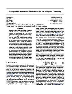
Fig. 1. WER as function of dimension showing the precision constrained models achieves significant fraction of improvement from MLLT to full covariance (while maintaining the same per Gaussian cost as the MLLT systems).
�
and precision matrices constrained to a � � � dimensional subspace. The subspace basis . $0/ was obtained using the modified Frobenius approximation of section IV-C, where the � � were taken to be those of the full covariance statistics model FC � � � � . Figure 1 shows that the PCGMM models achieve a significant fraction (e.g. �� � in � 7 dimensions) of the total improvement possible in going from MLLT to full covariance, while maintaining the same per Gaussian computational cost as the MLLT system. The figure also shows that the optimal performance is obtained with � LDA features, independent of the type of precision constraint. Including more LDA features degrades performance, which we will discuss further in section V-E. Apart from section V-E, we restrict all experiments in the remainder of the section to use the � 7 dimensional LDA projected features.
�
�
B. Result Obtained by Varying Model Size One of the many possible parameters to vary in selecting an acoustic model is the number of parameters per Gaussian. We have already seen that significant improvement can be obtained with 10K Gaussians by going from MLLT models to full covariance or precision constrained models, all with the same number of Gaussians. The reader may wonder how much of that same improvement could have been obtained simply by increasing the number of Gaussians. Table II is an attempt to answer that question. It gives word error rates for MLLT and full covariance models of various sizes, all based on the features from the � 7 dimensional LDA projection matrix LDA � � 7 � . The table shows that we could obtain much (but not all) of the full covariance gains using very large diagonal models, but that it requires very many parameters to do so, whereas the precision constrained approach can get similar gains with far fewer parameters. To build the models in the table, we needed to have a way of distributing the total number of Gaussians in a model among the different context dependent states. The simplest approach is to assign the same number of Gaussians to each state. However, a somewhat more principled, but still tractable, approach based on the Bayesian Information Criterion (BIC)
�
<%>�?
�� �
� � � ;
�
�
7
�
� � � < >@? �
�
� �
(80)
�
compoHere � is � the maximum likelihood model with � nents, � � is the number of parameters that model has, � and is called the penalty weight. Performing the Gaussian approximation to the Bayesian integral around � the � (maximum 3 . Including likelihood) critical point leads to the value of � a Gaussian prior on the model parameters results in larger � � values for ; so varying provides a natural way to obtain a one parameter family of choices for the state dependent � number of Gaussians � . To obtain the models in Table II, we trained models which are diagonal in the MLLT basis of the model MLLT � � 7 � described above, and which have a size that optimizes the BIC � criterion function (80) for various values of the BIC penalty . To reduce computational overhead (which was already several computer-years of time), the number of Gaussian components for lines in the table whose BIC penalty is marked with an asterix was calculated by extrapolating the number of components determined for larger BIC penalty values. The full covariance models have the same number of components for each state as the MLLT model on the same line. The error rates for the systems with 10K Gaussians in Table II are 7 - � and 3 - � � , which are quite close to the error rates of 7 - � � and 3 - � � for the 52-dimensional MLLT and full covariance models in Figure 1. The latter model has 3 7 � D Gaussians which are distributed among the states using BIC at previous stage of processing. This serves as a “sanity check” that the distribution of Gaussians from the previous BIC calculation, which we use for all experiments in this section apart from those in Table II, is reasonably good. Notice that the error rate of the full covariance model with just 10K Gaussians is significantly better than that of the MLLT model with 600K Gaussians, even though the full covariance model has only about one eighth as many parameters. The full covariance model with 60K Gaussians offers further WER improvements still. C. Exploring Precision Constraints Table III reports word error rates for 52 dimensional systems with unconstrained means and various constraints on the precision subspace. In all of the models the subspace for the precision matrices were computed based on the EM utility function using the statistics of the full covariance model FC � � 7 � . The final models were obtained by training the untied parameters by iterating EM on the training data to convergence. The table reports result for varying subspace dimension � , with the last row being the full covariance limit.
JOURNAL OF LATEX CLASS FILES, VOL. 1, NO. 11, NOVEMBER 2002
nGauss 5000 10000 19999 30001 42993 60144 79990 110818 142622 149709 210666 255626 350286 428770 609100
BIC penalty 35.180 15.110 6.910 4.457 3.000 2.250 1.744 1.305 1.000 1.000 0.770 0.670 0.500 0.354 0.250
MLLT WER 3.48% 2.68% 2.21% 2.15% 2.00% 1.95% 1.87% 1.83% 1.74% 1.76% 1.73% 1.72% 1.68% 1.68% 1.65%
11
FC WER 1.83% 1.56% 1.45% 1.42% 1.35% 1.34% 1.35%
D 0.25d 0.5d d 2d 4d 8d 26.5d
1.54%
stacked – – 2.67 2.35 2.01 1.82 –
EMLLT ML – – 2.67 2.04 1.81 1.65 1.58
PCGMM mod. frob ML 2.70 2.50 2.25 2.23 1.97 1.96 1.75 1.75 1.65 – 1.64 – 1.58 1.58
affine 3.05 2.89 2.42 2.06 – – –
TABLE III WER COMPARISON OF MODELS FOR LDA � ��� �
FEATURES WHICH HAVE
) . M ODELS ARE : EMLLT WITH STACKED BASIS AND ML TRAINED BASIS ,
PRECISION MATRICES CONSTRAINED TO A SUBSPACE OF DIMENSION
AFFINE
EMLLT WITH ML TRAINED BASIS , PCGMM WITH BASIS FROM F ROBENIUS ALGORITHM AND ML TRAINED BASIS .
MODIFIED
TABLE II WER OF MLLT AND FULL COVARIANCE MODELS ON THE LDA � ��� FEATURES . T HE NUMBER OF G AUSSIANS FOR EACH STATES WAS TRAINED �
USING
BIC FOR THE MLLT SYSTEMS USING VARIOUS BIC PENALTY
VALUES ( AND SOME EXTRAPOLATION IN THE CASE OF LINES WITH AN ASTERIX ).
The models in the “stacked” column in Table III are EMLLT models where the matrix D whose columns are the rank ) ) ) + one directions . $0/ for the precision matrices . $ $ / are obtained by “stacking” MLLT matrices for various phone classes (which forces � to be a multiple of � ). Preliminary experiments on the method used to generate the phone classes (manual vs data-driven) showed no significant differences in performance. Models for the second column of results in the table have ML trained EMLLT basis, seeded by the stacked bases and ) trained by updating the $ one at a time. The next column reports results for affine EMLLT models with the affine shift Z fixed to be the inverse of the (weighted) mean of the covariance matrices of the full covariance model and the rank ) one vectors $ trained by ML. The last two columns report results for PCGMM models where the subspace containing the precision matrices for all Gaussians (i.e. the basis of full covariance matrices . $ / ) was trained using the modified Frobenius approximation (next to last column) and maximum likelihood (last column). We make the following observations: The WER goes smoothly down to the full covariance result as the basis size increases. Models with an arbitrary precision subspace constraint perform much better than comparable size EMLLT models (which restrict the subspace basis to consist of rank one matrices), except of course when the basis size becomes big enough that one is almost obtaining the full covariance results. For the EMLLT models, the ML training of bases and the “stacked” bases are the same for ordinary MLLT � (� � ) and would be the same for full covariance � if the stack model were defined in that case, but for intermediate values we see that ML training essentially reduces the number of parameters required to model the covariance by half. On the other hand, for the general bases (PCGMM) case, maximum likelihood training does
�
�
�
�
�
not provide any significant gain over the seed model from the modified Frobenius algorithm, unless one goes � -7 � � . (Since down to a basis size as small as � the gain should only go down as � increases, we didn’t bother computing the ML trained PCGMM models with � 9 7 � .) Including an affine basepoint for the EMLLT basis leads to a significant improvement for the EMLLT models with � � � , � but already by the time the EMLLT basis is of 7 � , including the affine basepoint yields no size � gain. (Since the gain should only go down as � increases, we didn’t compute the affine EMLLT models for � 9 7 � .) The final stage of training for each of the models above consisted of training the untied parameters to convergence. The initial point for that training was a model trained solely based on the statistics of the full covariance model FC � � 70� which may be viewed as a “compressed” version of the full covariance model. It turns out that the compressed models were in fact rather close to the final model obtained after allowing the untied parameters to “see” all of the training data. Only in cases when the subspace dimension is very low (so that the compressed model is very far from FC � � 70� ) did the final training of the untied parameters have an appreciable effect. In those cases we might hope to gain some improvement by allowing the untied parameters to see the training data (and not just the model FC � � 7 � ). To test this, we collected full covariance EM statistics for the ML trained PCGMM � -7 � model with � � and retrained both the tied an untied parameters based on those statistics. This reduced the word error rate from 7 - � � to 7 - � � � . �
D. Dimensional Reduction with SCGMM and SPAM models The experiments so far in this section have shown the benefit of restricting precision matrices to a tied subspace. We now turn to experiments which restrict the linear weights as well. Results of these experiments are presented graphically in Figure 2 and numerically in Table IV. The table and graph give word error rates for various types of models, as a function of the number of untied parameters per Gaussian. All systems in any one row have roughly the same total number of parameters
JOURNAL OF LATEX CLASS FILES, VOL. 1, NO. 11, NOVEMBER 2002
12
5
�
�
��
�
�
The improvement of the SPAM � models with ML trained basis over the seed models SPAM Z becomes significant for small basis sizes. The SPAM � models which constrain the precision and linear weights of a � 7 dimensional model to dimension � � have significantly lower WER than the equally costly PCGMM models on the LDA projected features vectors. The latter models are, as we have already seen, better than the corresponding MLLT models. The general subspace constrained (SCGMM) models, yield still further improvements over the SPAM � models with comparable cost. As one example of the combined gains, note that the model SCGMM � � 7 7 � obtains a comparable error rate (about 7 - � � ) as the model MLLT � � 70� which has four times as many parameters per Gaussian and D - � times as many total parameters.
�
�
�
�
�
�
The astute reader may question whether or not the improvements obtained in allowing an arbitrary subspace constraint could have been obtained by still sticking with SPAM models in which the dimensions � of the precision and � of the linear weight subspaces are allowed to vary, as long as the total dimension � 1 � is held fixed. Table V addresses this. It compares the general subspace constrained GMM with a 7 dimensional feature space to ML trained SPAM models, also with a 7 dimensional feature space. It is interesting to note that in this case we obtained improvement in the SPAM
3
2.5
15
20
25
30
35
40
45
50
55
dimension d1 of linear and quadratic feature space
Fig. 2. Comparison of word error rates for various types of subspace constrained Gaussian mixture models as a function of half the subspace dimension (which is the dimension of both the linear and quadratic subspaces when they are separately defined). Plot shows that the more general the model and the more completely the model is trained to maximize likelihood, the better the WER becomes. This plot is graphical version of Table IV (not including first line of table). ��9 8 13 20 39 52
�� �
3.5
1.5 10
�
�
SCGMM(d=52, F=2*d1)
4
2
�
��
MLLT(d1) PCGMM(d=d1, D=d1) SPAM0(d=52, D=d1,L=d1) SPAMML(d=52, D=d1,L=d1)
4.5
word error rate in percentages
(and computational cost) since the tied parameters contribute only a small fraction to the total. All models are built on the � 7 dimensional acoustic vectors produced by LDA � � 70� . The next paragraph describes how each of the five types of models were trained. In all cases, after the tied subspace constraints were determined, the untied parameters were trained by iterating the EM algorithm to convergence. The models, in order of increasing accuracy are as follows. The models labeled MLLT or MLLT � � � � are the same as appearing in Figure 1, namely MLLT model built on the � 7 . (These LDA projected vectors in dimension � � for � � models may be considered models for vectors produced by LDA � � 7 � since the projection matrix LDA � � � � from 3 3�� to � � dimensions is the composition of the projection from 3 3�� to � 7 dimensions with the projection from � 7 to � � dimensions.) The � � � �� models labeled PCGMM or PCGMM � � � � � also appear in Figure 1. They are models on the LDA � � � � vectors with a � � -dimensional precision basis obtained � � 7 by� modified � � � � �� Frobenius training. The models SPAM Z � � � � � have the seed precision subspace that optimizes the modified Frobenius approximation
and the seed linear weight function when holding the subspace which optimizes the precision subspace fixed. The SPAM � models are obtained from the SPAMZ models by further ML training of the basis � (based on statistics of X � � � 70� ). Finally, the SCGMM � � � 7 � � � models are Gaussian mixture models with the � 7 X exponential weights constrained to a subspace of dimension 7 � � obtained by maximum likelihood training, seeded by the SPAM � models. We observe the following:
�
MLLT 4.92 3.71 2.85 2.67
PCGMM 4.58 3.18 2.14 1.97
SPAM 4.12 3.06 2.13 1.97
�
� �
SPAM 4.69 3.26 2.59 2.10 1.96
SCGMM 3.42 2.71 2.35 1.95 1.90
TABLE IV WER TABLE FOR : � 9 - DIMENSIONAL MLLT AND PCGMM MODELS AND � - DIMENSIONAL SPAM MODELS ( WITH SEED AND ML TRAINED BASES ) AND GENERAL SUBSPACE CONSTRAINED MODELS HAVE SEPARATE
(SCGMM) MODELS . A LL
��9 - DIMENSIONAL SUBSPACES FOR LINEAR
WEIGHT AND PRECISION MATRICES , EXCEPT FOR WHICH HAS A COMBINED
SCGMM MODELS
� ����9 DIMENSIONAL SUBSPACE .
model by allowing more untied parameters to be invested in the precision subspace than in the linear weights subspace. However, allowing a general subspace constraint yields even better results and obviates the need to optimize over � for fixed � 1 � . E. Concerning degradation in 3 3�� dimensions As we’ve seen already from Figure 1, the MLLT, full covariance, and precision constraint models all degrade when they model LDA projected vectors with more than about � features. This is despite the fact that they all use only 3 9 Gaussians and we know from the BIC experiments in section V-B that full covariance models in dimension � 7 don’t start to degrade significantly due to overtraining until they have at Model Type SPAM(d=52,D=8,L=18) SPAM(d=52,D=13,L=13) SPAM(d=52,D=18,L=8) SCGMM(d=52,F=26)
WER 3.52 3.26 3.00 2.71
TABLE V C OMPARISON OF SCGMM AND SPAM MODELS WITH THE SUBSPACE DIMENSION .
SAME TOTAL
JOURNAL OF LATEX CLASS FILES, VOL. 1, NO. 11, NOVEMBER 2002
13
least 9 Gaussians. So the degradation when increasing the LDA dimension up to 303�� (which one might expect in the � 3 3�� 5 � 7 times as full covariance case to require about 7 - 7 � 7 � dimensional models) many data points per Gaussian as the is probably not due to a lack of training data, but simply the fact that the extra features are not informative. To explore this just a little bit further, we performed a couple of additional experiments. First of all, we “lifted” � �7 � 7 � X the model SCGMM � � to 303�� dimensions (by including the LDA projection terms) and used that as a seed to obtain an ML trained model SCGMM � 3 3�� 7 � � in 3 3�� dimensions with a 7 � dimensional subspace constraint. The error rate of 7 - �,3 � for SCGMM � � 7 7 � degrades to D - 3� � for SCGMM � 303�� 7 � . On the other hand the analogous degredation in error rate in the MLLT case, from 7 - � � for the model MLLT � � 70� of Figure 1 to 7 - 3 � for MLLT � 303�� � was not as bad. We conclude that maximum likelihood training of the tied parameters in going from SCGMM � � 7 7 � to SCGMM � 3 3�� 7 � � seems to be “learning” to look at components of the LDA projected vector which are providing noise rather than information. On a qualitative level, there seem to be at least two contributing factors to the degradation that comes from looking at the noisy LDA directions. On the one hand, the part of the model in the noisy directions could itself be degrading system performance. On the other hand, the model in the non-noisy directions could be degraded because ML training is having it’s “attention taken away” from the clean directions. To try to sort this out, we did some additional experiments. Table VI reports the results. The first two lines of the table give the WER for the fully EM trained � 7 and 3 3�� dimensional full covariance models seen already in Figure 1. The model of the third line was the full covariance model in 303�� dimensions obtained from the E-step statistics of FC � � 70� . The model on the final line of Table VI was a 3 3�� dimensional full covariance model with block diagonal covariance matrices where the part of the means in the first � 7 dimensions were taken from FC � � 7 � , while the complementary parts were taken from the E-step statistics above. Since the last model in the Table VI, whose Gaussians are a product of Gaussians from FC � � 7 � with Gaussians in the noisy directions, didn’t suffer from the problem of degradation of the non-noisy directions, we can conclude that the part of that model in the noisy directions is what is causing the degradation. The fact that the models in the last three lines of the table have about the same performance (in total, although their breakdowns by test condition differ more) suggests that the problem of degradation of the non-noisy part of the model is less severe.
Model FC � ��� FC � / /�� � / �/ � dimensional stats of # � � ��� # � � ��� + complimentary stats �
�
�
WER ���� / ; � � / ; � � � / ; / �� � / ; �
TABLE VI C OMPARISON OF WER FOR SOME FULL COVARIANCE MODELS DESCRIBED IN S ECTION V-E.
�
�
�
�
�
�
F. Additional Complexity Reduction Techniques We conclude with two experiments showing that the precomputation cost and number of Gaussians that need to be evaluated for a subspace constrained model can be reduced greatly without taking too much of a performance hit. We will reduce the precomputation cost by using a hybrid model
as defined in (20). The number of Gaussians that we need to evaluate will be reduced by using a Gaussian clustering technique [35]. These experiments were first reported on in [18], which the reader can refer to for further details. � � � Table IV shows that the model � � � � � D� � D� � 7 7 has error rate - 3 � � . A comparable error rate of - 35D � � � is obtained from a hybrid model Hybrid � � D� � � � � 9 in which the basis matrices $ are each a D� 3 � � linear combination of 9 3 rank one matrices. The model was trained to maximize likelihood by the techniques of [17]. This comparable error rate was obtained by balancing the small degradation due to the constraint on the $ with the small improvements due to the fact that an affine Z was included and the $ were trained in a true maximum likelihood fashion. The model reduces the feature precomputation cost from � � � � 1�3 �6587�� D to 9 � 1 � 9 � 3 7 . Next, we cluster the Gaussians of the hybrid model using a variant of K-means clustering that uses the KullbackLiebler distance between Gaussians. We thus produce 3 7 � cluster centers, each of which is represented by a Gaussian (constrained by the hybrid model subspace) and a map from Gaussians of the hybrid model to cluster centers. When evaluating a model, we first evaluate all of the cluster center Gaussians and use the top rankings one to choose 3 Gaussians of the hybrid model to evaluate, with the unevaluated Gaussians replaced by a simple threshold value. This causes the error rate to increase to 7 - 3� � , but reduces the number of Gaussian evaluations required from 3 7 � D to 7 7 � . Although the memory cost has been increased a little bit, the evaluation time cost (gotten by multiplying by � , the 9 number of parameters per Gaussian) reduces from about 9 to about 3 � .
�
�
�
�
�
�
�
VI. L ARGE VOCABULARY C ONVERSATION S PEECH R ESULTS All of the experiments in section V were performed on a collection of small vocabulary, grammar based tasks. Although we tried to explore both low cost and high cost regions of the parameter space of models, one thing that we did not do was vary the number, � , of context dependent states. We also did not consider speaker adaptation. Also, the test set we used was not an industry standard set. These issues are addressed in [20], where we obtained gains using precision constrained models in the unconstrained resource case on several tasks in the IBM superhuman speech corpus [22]. For completeness, we briefly summarize here some of the results obtained on the part of the superhuman corpus consisting of the switchboard
JOURNAL OF LATEX CLASS FILES, VOL. 1, NO. 11, NOVEMBER 2002
� � >��� � � > "4)� � >�� � � > "4)� / � >�� � � > "4)�?� >�� � > "4)� / � >��
model MLLT �(� PCGMM ��� PCGMM ��� PCGMM ��� PCGMM ���
�
WER �� � � ; � � � ; � � � / ; � �� � / ; ��� � > ; �
�
FM
TABLE VII R ESULT ON
SWITCHBOARD
98 CORPUS FOR : MLLT BASELINE , PRECISION
) 0��"$� ��" � ,
CONSTRAINED MODELS WITH SUBSPACE DIMENSION OF
�0�
AND
FMLLR+MLLR ADAPTATION OF THE )
HAD
� /�� 6
�
� MODEL . A LL MODELS
G AUSSIANS . A LLOWING ANY NUMBER OF G AUSSIANS FOR AN
� MLLT MODEL PRODUCED AT BEST A WER OF � � ; .
portion of the 1998 Hub 5e evaluation set, which consists of 3 35D minutes of audio. We started by training baseline MLLT models of various sizes using BIC, similarly to how it was done in V-B. Training data consisted of 247 hours of Switchboard data and 17 hours of CallHome English, all released by the LDC. All models had � ��: dimensional � context dependent states and use data vectors obtained by LDA projection of 7 3 dimensional vectors, which were themselves obtained by concatenating consecutive vectors of mean normalized, 7 � dimensional MFCC features. Speaker adaptive VTLN warping factors [36], and FMLLR transformations [37] were trained based on an initial decoding. A trigram language model with D�� 9 words was used. We took as our baseline model, the one with the BIC penalty of 3 and 7 3�� 9 Gaussians, which had an error rate of D 7 - � . (The lowest WER of D 7 - � � was achieved with D � � 9 Gaussians, while going up to 3�� 9 Gaussian degraded performance to D 7 - � � .) We calculated modified Frobenius basis direction $ based on the statistics of a 3 9 Gaussian full covariance model. An MLLT model with this number of Gaussians had an error rate of D � - D � , which improved to D�D - � � with full covariance modeling. The precision constrained model with equal per � Gaussian cost as the MLLT model (i.e. � ), had an error rate of D � - � � , which splits the difference. Next, we trained a precision constrained model with the � same � basis as above, but with 7 3�� 9 Gaussians as in the baseline model. This gave a very small improvement over the baseline model. However, we expect that a little more gain would have been obtained if we had trained the basis by maximum likelihood and based on the full 7 3�� 9 statistics (which would have been rather painful). We were able to gain better improvements over the MLLT baseline by increasing the precision subspace size to 3 7 and 7 � . We obtained further performance gains by MLLR and FMLLR speaker adaptation which were comparable to the performance gains when those techniques were used with MLLT models based on different � 7 features (as can be seen from Table 2 of [22]). with � 3 . The result of all these experiments appear in Table VII.
�
VII. D ISCUSSION The general picture that emerges from our experiments on both small vocabulary, grammar based tasks and large vocabulary conversational speech tasks is that the best performance
14
is obtained by restricting to features that have information rather than noise and employing full covariance Gaussian mixture models rather than diagonal models, even diagonal models with a huge number of Gaussians. Although, the full covariance models are very expensive to evaluate and train, they can be usefully approximated by mixtures of Gaussians which place a subspace constraint on the precision matrices and linear weights of all the Gaussians. Models with larger subspace dimension have the lowest error rates. We have explored various types of specialization of the general subspace constraint to compare their performance/cost operating curves. In particular the very successful combination of LDA projection with MLLT (and in fact EMLLT) models is one specific specialization. We have found that the more general the subspace constraint and the more completely the model is trained to maximize likelihood, the better the operating curve. We have seen that these models can be combined successfully with the techniques of speaker adaptation (to reduce the error rate) and clustering (to reduce the acoustic model evaluation time). We have tried to present a fairly thorough and self-contained discussion. However many other techniques and combinations of techniques are left to be explored. For example, we have not considered here models in which the Gaussians are clustered and there is a separate subspace restriction for each cluster, rather than a globally tied subspace. Perhaps because we have tried to present a picture that unifies many different previous approaches, the reader may be left feeling that we have added more parameters to the already bewildering task of finding the best model given some resource constraints. One possibility is to choose the model (i.e. number of Gaussians per state, type of subspace constraint, semi-tied clustering, clustering to reduce number of Gaussian evaluations, the choice of subspace types and dimension, ...) which maximizes training likelihood. With a few additional tricks and shortcuts, this just might be practicable with the computational power available today. On the other hand, we could also try to choose a criterion other than maximum likelihood. In fact, in [23] we showed that futher gains are possible with these subspace constrained models using discriminative training techniques. We intend to explore this futher in the future [24]. A PPENDIX I S IMPLE P ROPERTIES OF E XPONENTIAL M ODELS We first give some background about distributions in the exponential family. For further detail, see, for example, [38]. An exponential model � �� associated with feature �� , B � � � � � B � ��� � - - - B � ��� � � , and function B�� � � @A � C � - - - C � � � is the probability density weight vector C "VR "SR R function R (�T@�%$�
(�T@�%$5 )2#6 � T57
D EFINITION
AND
� �
� �
� T57
�
��� �
where
5 � � B
9
� �B �B
�C
�C �
� � �
�$ ;
�C
"SR
< >@?
� �
�
(81)
(�T@�%$�
� � � B
�C
(82)
��
(83)
JOURNAL OF LATEX CLASS FILES, VOL. 1, NO. 11, NOVEMBER 2002
15
is a normalization constant and its negative logarithm. When there is no danger of ambiguity, we write � � C � and 9 � C � as shorthand for � � B C � and 9 � B C � . The weight vector C is required to belong to the “natural parameter space” � B � , consisting of the weight vectors for which the normalization constant is finite:
�
�
� B � � .�C � � � B
��
�C �
/ -
��� Given a set of training sample � ��� - - - � � + � , let � � be � � the distribution on consisting of equally weighted point � � R the mean log-likelihood of the � under masses at the � . Then
the distribution �
� T57
(84)
is:
�
#
�3
�C � . � �/ � �
�
+ C
<%>�?
R � T57
� � �! ��� �� � B � 1
�� �� 9
(85)
�C �
(86)
Exponential distributions have several well known properties, including the following: 1) The gradient of R <%>�? � � C � equals the mean of B under the � T57
distribution R the Covariance matrix 2) The Hessian of <%>�? � � B C � equals � T57
of B under the distribution . 3) <%>�? � � B C � is convex in C . 4) � B � is a convex set. � 5) The mean log-likelihood function � � C � . � / � is concave in C . The maximum likelihood weight vector C for the � training data . � / is uniquely determined by the zero gradient condition:
�
�
�
� � �! ��� �� � B
��� � � ;
� ����� ��� � � � B
��� � �
�
(87)
i.e. by the condition that the training expectation of the features equals the model expectation of the R features. � T57
6) The maximum likelihood distribution associated � with training data . � / is also the unique probability density function ���� � on � which maximizes the ; $ �� � entropy < >@? � � � subject to the constraint that �B �� �� � �B �� ��. Note that the convexity of < >@? � and the concavity of � follow immediately from property 2 above and the fact that the covariance matrices are positive definite. (Ok, we’re ignoring the possibility of degeneracies here.) The fact that the set � B � is convex follows because the function � � B C � is convex in C . This, in turns follows either from the fact that < >@? � is convex � � C + B � � � � is convex in C and or directly from the facts integration is linear.
��
��
��
�
�
A PPENDIX II I NITIALIZATION OF U NTIED PARAMETERS
�
�
�
�
�"� !
�
�
�
�� �
�
��
"
*
�
� ��
�
�
�
�
#!� !
%$ ! �
#� � �3 �% �'&)(
!
�
��
�+* �
�
��
" "
��
+�
�
(88)
where . / and . / are the eigenvectors and corresponding � � � eigenvalues of . The POCS theorem guarantees that, if � � � � � is non-empty, then the sequence converges � to� ac2 point in � . Then there� exists some such that ; � c2 � � 3 and thus is � strictly positive � @2 � definite. Since is also an element of , the algorithm converges in a finite number of steps. other hand, if � � � On@2 the � ; � is empty, then the sequence � decreases from above to a positive lower bound � . In practive, the algorithm should terminate with a failure if becomes � @2 � too large, � is no longer decreasing significantly, and still fails to be positive definite. To handle the case when Z is non-zero, we define the closed, convex sets �
��
-, � /. 0 �� 1. 0 � ��
�
��
�
�
This appendix provides an algorithm which determines a positive definite matrix within a given affine subspace of the space of � � � � symmetric matrices (or shows that no such point exists). That is, given the tied parameters, a basepoint Z and a basis . $ / !$&% � , we show how to find untied $ $ parameters
! so that the matrix � � Z 1 $ is positive ' ' definite. In the body of the paper, we have restricted ourselves to cases where the solution is obvious because either one of
�
�
�
� � �! ��� ��
����
�
�
the $ is positive definite or a subset of the $ consists of rank one matrices whose directions form a basis of � . We handle the general case in this appendix with a simple adaptation of the method of alternating Projections Onto Convex Sets (POCS). The POCS theorem [39]–[41] states that if there is a point in the intersection of two closed convex sets (both contained in a suitable metric space), then the point can be found from an arbitrary initial point, by alternatively projecting� on one space and then the other. The
projection of a matrix onto a convex set, is the matrix � in the convex set that minimizes the distance to the matrix . The distance function we use here is the one induced from the Frobenius norm. Applying POCS naively to our problem, we obtain a � (73) and the point in the intersection of our affine space space of non-negative matrices. Unfortunately, we could well obtain the zero matrix. Also, the algorithm does not converge in a finite number of steps. We modify the naive algorithm so as to avoid these problems by replacing the non-negativity condition by a threshold on the smallest eigenvalue. It is simplest to first describe the algorithm to find a positive � definite point in in the case when the affine shift Z � � �� . � :&3 3 / vanishes. Let be the (closed, convex) set of symmetric matrices whose minimum eigenvalues is greater than or equal to : . � Also let be the (closed, convex) intersection of and , and let and be their respective interiors. Our goal is to find a point in Z , but it is easy to see, using the fact that Z is a cone, that finding a point in Z is equivalent to finding a point in � Z . To � find such a point, we start with an initial symmetric matrix Z (e.g. the inverse � � � covariance matrix which we are trying to approximate) � and then alternatingly project on the set � and � to obtain a � � � 3 - - - , where is in� sequence , : for : odd and � is � c2 �
in � for : 9 even. The projection of onto � � � onto is a simple linear projection. The projection onto � � is the matrix
0 �� .
��
�
0
��
�
32 �2
�
�
� �
.
� � #! $ � $ � ! $% Z ' ' 2, � � 2
�
� '
Z
�43 /
(89) (90)
JOURNAL OF LATEX CLASS FILES, VOL. 1, NO. 11, NOVEMBER 2002
2
16
By multiplying by a scalar, points in � determine positive � definite points in , and the converse is true as well. Similarly to above, we can use POCS to determine � a point in � by alternating between projection onto � and . The projection � � c2 � � of onto is given by:
��
��
�
2 �� $ � if � 3 Z ! � ' !$&% Z !$ � $ otherwise. ' 2 2' � �
! � have components: Here ! ! and ! ' ' #! � � � � ��� �� ; � �� $ � � � ! $!� N�O Z !$ �% � ' 2 � � # ! � 2 � � $� � � � � � � � $ � � � ! N�O !$ �% Z ' 2 matrix of inner products N�O �� � $ � � � , � where � ! is the 3 � � and � ! � is the matrix of inner products for � � ---� .
�
� �c2
�
� � !$&% Z Z 1
!$
2
2
2
(91)
(92)
(93)
�
� �� �
�
ACKNOWLEDGMENT We are grateful to the members of the IBM “Superhuman team” for discussion, models, lattices, code, and all that, in particular to Brian Kingsbury, George Saon, Stan Chen, and Lidia Mangu. We also would like to thank Charles Micchelli for useful mathematical discussions. R EFERENCES [1] D. B. Rubin and D. Thayer, “EM algorithm for ML factor analysis,” Psychometrika, vol. 57, pp. 69–76, 1976. [2] C. Bishop and M. Tipping, “Probabilistic principal component analysis,” J. of the Royal Statistical Society, Series B, vol. 21, no. 3, pp. 611–622, 1999. [3] L. K. Saul and M. G. Rahim, “Maximum likelihood and minimum classification error factor analysis for automatic speech recognition,” IEEE Transactions on Speech and Audio Processing, vol. 8, no. 2, pp. 115–125, 1999. [4] R. A. Gopinath, B. Ramabhadran, and S. Dharanipragada, “Factor analysis invariant to linear transformations of data,” in Proc. ICSLP, 1998. [5] S. Dharanipragada and K. Visweswariah, “Covariance and precision modeling in shared multiple subspaces,” in Proc. ICASSP, 2003. [6] R. Gopinath, “Maximum likelihood modeling with gaussian distributions for classification,” in Proc. ICASSP, 1998. [7] M. J. F. Gales, “Semi-tied covariance matrices for hidden Markov models,” IEEE Transactions on Speech and Audio Processing, 1999. [8] P. Olsen and R. A. Gopinath, “Modeling inverse covariance matrices by basis expansion,” in Proc. ICASSP, 2002. [9] ——, “Modeling inverse covariance matrices by basis expansion,” IEEE Transactions on Speech and Audio Processing, to appear. [10] R. Fisher, “The use of multiple measurements in taxonomic problems,” Ann. Eugen., 1936. [11] ——, “The statistitical utilization of multiple measurements,” Ann. Eugen., 1938. [12] C. Rao, Linear Statistical Inference and Its Applications. John Wiley and Sons, 1965. [13] N. Campbell, “Canonical variate analysis - a general formulation,” Australian Journal of Statistics, 1984. [14] N. Kumar, “Investigations of silicon auditory models and generalization of linear discriminant anlysis for improved speech recognition,” Ph.D. dissertation, Johns Hopkins University, March 1997. [15] N. Kumar and A. G. Andreou, “Heteroscedastic discriminant analysis and reduced-rank HMMs for improved speech recognition,” Speech Comm., vol. 26, pp. 283–297, 1998. [16] S. Axelrod, R. A. Gopinath, and P. Olsen, “Modeling with a subspace constraint on inverse covariance matrices,” in Proc. ICSLP, 2002.
[17] K. Visweswariah, P. Olsen, R. A. Gopinath, and S. Axelrod, “Maximum likelihood training of subspaces for inverse covariance modeling,” in Proc. ICASSP, 2003. [18] S. Axelrod, R. A. Gopinath, P. Olsen, and K. Visweswariah, “Dimensional reduction, covariance modeling, and computational complexity in ASR systems,” in Proc. ICASSP, 2003. [19] K. Visweswariah, S. Axelrod, and R. Gopinath, “Acoustic modeling with mixtures of subspace constrained exponential models,” in Proc. Eurospeech, 2003, to appear. [20] S. Axelrod, V. Goel, B. Kingsbury, K. Visweswariah, and R. Gopinath, “Large vocabulary conversational speech recognition with a subspace constraint on inverse covariance matrices,” in Proc. Eurospeech, 2003, to appear. [21] V. Vanhoucke and A. Sankar, “Mixtures of inverse covariances,” in Proc. ICASSP, 2003. [22] B. Kingsbury, L. Mangu, G. Saon, G. Zweig, S. Axelrod, V. Goel, K. Visweswariah, and M. Picheny, “Toward domain-independent conversational speech recognition,” in Proc. Eurospeech, 2003, to appear. [23] V. Goel, S. Axelrod, R. Gopinath, P. Olsen, and K. Visweswariah, “Discriminative estimation of subspace precision and mean (SPAM) models,” in Proc. Eurospeech, 2003, to appear. [24] S. Axelrod, V. Goel, R. A. Gopinath, P. Olsen, and K. Visweswariah, “Discriminatively trained acoustic models comprised of mixtures of exponentials with a tied subspace constraint,” in preparation. [25] N. K. Goel and A. G. Andreou, “Heteroscedastic discriminant analysis and reduced-rank HMMs for improved speech recognition,” Speech Comm., vol. 26, pp. 283–297, 1998. [26] L. Vandenberghe, S. Boyd, and S.-P. Wu, “Determinant maximization with linear matrix inequality constraints,” SIAM J. Matrix Anal. Applic., vol. 19, no. 2, pp. 499–533, April 1998. [27] E. Polak, Computational Methods in Optimization: A Unified Approach. Academic Press, 1971. [28] J. N. D.C. Liu, “On the limited memory BFGS method for large scale optimization problems,” Mathematical Programming, vol. 45, pp. 503– 528, 1989. [29] F. Tisseur, K. Meerbergen, “The quadratic eigenvalue problem,” Society for industrial and applied mathematics, vol. 43, no. 2, pp. 235–286, 2001. [30] S. Deligne, E. Eide, R. Gopinath, D. Kanevsky, B. Maison, P. Olsen, H. Printz, and J. Sedivy, “Low–resource speech recognition of 500 word vocabularies,” in Proceedings of the Sixth European Conference on Speech Communication and Technology, Aarhus, Denmark, September 2001. [31] L.R. Bahl et al., “Performance of the IBM large vocabulary continuous speech recognition system on the ARPA Wall Street Journal task,” in Proc. ICASSP, 1995. [32] G. Saon, M. Padmanabhan, R. Gopinath, and S. Chen, “Maximum likelihood discriminant feature spaces,” in Proc. ICASSP, 2000. [33] G. Schwarz, “Estimating the dimensions of a model,” Annals of Statistics, 1978. [34] S. Chen and R. A. Gopinath, “Model selection in acoustic modeling,” in Proc. Eurospeech, 1999. [35] E. Bocchieri, “Vector quantization for efficient computation of continuous density likelihoods,” in Proc. ICASSP, 1993. [36] H. Hermansky, “Perceptual linear predictive (PLP) analysis of speech,” Journal of the Acoustical Society of America, vol. 87, no. 4, pp. 1738– 1752, April 1990. [37] M. J. F. Gales, “Maximum likelihood linear transformations for HMMbased speech recognition,” Cambridge University, Technical Report TR 291, 1997. [38] L. Brown, Fundamentals of Statistical Exponential Familes. vol 9 of Lecture Notes - Monograph Series, Institute of Math. Stat., 1991. [39] L. M. Bregman, “Finding the common point of convex sets by the method of successive projections,” Dokl. Akad. Nauk. USSR, vol. 162, pp. 487–490, 1965. [40] ——, “The relaxation method of finding the common point of convex sets and its application to the solution of problems in convex programming,” USSR Computational Math. & Math. Physics, vol. 7, no. 3, pp. 200–217, 1967. [41] L. G. Gubin, B. T. Polyak, and E. V. Raik, “The method of projections for finding the common point of convex sets,” USSR Computational Math. & Math. Physics, vol. 7, no. 6, pp. 1–24, 1967.