STRUCTURED ADAPTIVE MODEL INVERSION CONTROL WITH FAULT TOLERANCE AND ACTUATOR POSITION LIMITS

A Thesis by MONISH DEEPAK TANDALE

Submitted to the Office of Graduate Studies of Texas A&M University in partial fulfillment of the requirements for the degree of MASTER OF SCIENCE

December 2002

Major Subject: Aerospace Engineering

STRUCTURED ADAPTIVE MODEL INVERSION CONTROL WITH FAULT TOLERANCE AND ACTUATOR POSITION LIMITS A Thesis by MONISH DEEPAK TANDALE Submitted to Texas A&M University in partial fulfillment of the requirements for the degree of MASTER OF SCIENCE

Approved as to style and content by:

John Valasek (Chair of Committee)

John L. Junkins (Member)

Srinivas Rao Vadali (Member)

Suhada Jayasuriya (Member)

Ramesh Talreja (Head of Department) December 2002

Major Subject: Aerospace Engineering

iii

ABSTRACT Structured Adaptive Model Inversion Control with Fault Tolerance and Actuator Position Limits. (December 2002) Monish Deepak Tandale, B.E., V.J.T.I, Mumbai University Chair of Advisory Committee: Dr. John Valasek

Structured Adaptive Model Inversion (SAMI) is a model reference adaptive control formulation that takes advantage of the dynamical structure of the state-space descriptions of a large class of systems. Most dynamic systems can be broken into an exactly known kinematic level part, and a momentum level part with uncertain system parameters. The SAMI formulation enables the imposition of exact kinematic differential equations, and restricts the adaptation process that compensates for model errors to the acceleration level. Dynamic inversion is used to solve for the control The dynamic inversion is approximate, as the system parameters are not modelled accurately. Hence an adaptive control structure is wrapped around the dynamic inverter to account for uncertainties. In high performance dynamic systems the total number of actuators used may be greater than the number of states to be closely controlled or tracked. In the case of redundant actuation, it is still possible to closely track the desired states even if some of the actuators fail, as long as the number of active actuators is more than or equal to the number of states to be tracked. Therefore, if it is possible to reconfigure the control after failure, the stability and performance of the system can be maintained. The research presented in this thesis is the result of an attempt to provide fault tolerance, without the need of a fault detection algorithm, by extending the SAMI methodology.

iv

Traditional adaptive control lacks an adequate theoretical treatment for control in the presence of actuator saturation limits. The research presented in this thesis attempts to extend the adaptive control methodology to facilitate correct adaptation in the presence of actuator saturation. The central idea is to modify the reference trajectory on saturation, in such a way that the modified trajectory approximates the original reference as close as possible, and can be tracked within saturation limits. Results presented in this thesis for an inverted pendulum on a cart and nonlinear six degree of freedom simulation of an aircraft show that the synthesized control laws are able to handle parametric uncertainties, initial error conditions, actuator failures and actuator position constraints.

v

To my parents, for giving me a reasonably good open-loop dynamics via their genes and my teachers, who helped me put a closed-loop around it, to ensure stability and performance.

vi

ACKNOWLEDGMENTS

I would like to thank my committee chairman Dr. John Valasek for giving me an opportunity to pursue this research. I am grateful to him not only for his academic guidance but also for his continuous support and encouragement during the course of my research I thank my committee members Dr. John Junkins, Dr. Srinivas Rao Vadali and Dr. Suhada Jayasuriya for being a part of my committee and evaluating my research. I remain indebted to them for the strong fundamentals that they provided, in the courses that they taught me. I would also like to thank Dr. Swaroop for the mathematical foundation that he provided in nonlinear control, which helped me develop proofs for my adaptive control methodology. I thank the administrative staff of the Aerospace Engineering Department for their cooperation and help in administrative matters. I am grateful to colleagues for the fruitful discussions which gave me better insights into the research. I thank my friends for standing by my side in times good and bad. A special thanks to Kamesh Subbarao for guiding in my research from time to time and for being an inspiration and a role model. Finally, I thank my family for their continuous support, encouragement and love through all these years.

vii

TABLE OF CONTENTS

CHAPTER I

II

Page INTRODUCTION . . . . . . . . . . . . . . . . . . . . . . . . . .

1

A. Model Reference Adaptive Control . . . . . . . . . . . . . B. Structured Model Reference Adaptive Control . . . . . . . C. Structured Adaptive Model Inversion Control . . . . . . .

3 4 5

FAULT TOLERANT STRUCTURED ADAPTIVE MODEL INVERSION CONTROL . . . . . . . . . . . . . . . . . . . . . .

8

A. B. C. D. E.

Introduction . . . . . . . . . . . . . . . . . . . . . . . . . . Redundant Control and Actuation Failure Problem . . . . Strategies to Handle Actuation Failure . . . . . . . . . . . Mathematical Modelling of Actuator Freezes . . . . . . . . Mathematical Formulation of the Fault Tolerant SAMI controller . . . . . . . . . . . . . . . . . . . . . . . . . . . F. Stability Analysis . . . . . . . . . . . . . . . . . . . . . . . G. Example # 1: Control of the Inverted Pendulum on a Cart with Actuator Failure . . . . . . . . . . . . . . . . . . H. Nonlinear Six-Degree-of-Freedom Simulation of an F-16 type aircraft with Thrust Vectoring . . . . . . . . . . . . . 1. Definition of Variables and Development of a NonLinear Mathematical Model of the F-16 type Aircraft 2. Example # 2: Steady Level 1g Flight . . . . . . . . . 3. Example # 3: Steady Level Turn . . . . . . . . . . . . III

MODIFIED REFERENCE STRUCTURED ADAPTIVE MODEL INVERSION CONTROL WITH ACTUATOR SATURATION CONSTRAINTS . . . . . . . . . . . . . . . . . . . . . . . . . . . A. Introduction . . . . . . . . . . . . . . . . . . . . . . . . . . B. Control Saturation Limits and Problems Introduced in Adaptive Systems due to Saturation . . . . . . . . . . . . . C. Mathematical Formulation . . . . . . . . . . . . . . . . . . D. Numerical Example # 1 : Control of an Inverted Pendulum E. Numerical Example # 2 : Control of an Inverted Pendulum

8 8 9 9 11 19 20 28 28 33 38

45 45 45 47 54 59

viii

CHAPTER IV

Page CONTROLLER TO HANDLE COMBINED ACTUATOR FAILURES AND ACTUATOR SATURATION . . . . . . . . . .

63

A. Mathematical Formulation . . . . . . . . . . . . . . . . . . B. A Nonlinear Six-Degree-of-Freedom Simulation of an F-16 type Aircraft with Simultaneous Actuator Failure and Actuator Saturation . . . . . . . . . . . . . . . . . . .

63

65

V

CONCLUSIONS . . . . . . . . . . . . . . . . . . . . . . . . . . .

73

VI

RECOMMENDATIONS AND FUTURE RESEARCH DIRECTIONS . . . . . . . . . . . . . . . . . . . . . . . . . . . . .

75

REFERENCES . . . . . . . . . . . . . . . . . . . . . . . . . . . . . . . . . . .

76

APPENDIX A . . . . . . . . . . . . . . . . . . . . . . . . . . . . . . . . . . .

79

APPENDIX B . . . . . . . . . . . . . . . . . . . . . . . . . . . . . . . . . . .

81

APPENDIX C . . . . . . . . . . . . . . . . . . . . . . . . . . . . . . . . . . .

85

VITA . . . . . . . . . . . . . . . . . . . . . . . . . . . . . . . . . . . . . . . .

86

ix

LIST OF TABLES

TABLE

Page

I

Variation in the Parameters for the Inverted Pendulum on a Cart . .

23

II

The Error in the Initial Conditions for the Inverted Pendulum on a Cart 23

III

The Reference States for Steady Level Flight . . . . . . . . . . . . .

33

IV

The Reference States for Steady Level Turn . . . . . . . . . . . . . .

38

V

Variation in the Parameters for the Inverted Pendulum (Example 1)

57

VI

The Error in the Initial Conditions for the Inverted Pendulum (Example 1). . . . . . . . . . . . . . . . . . . . . . . . . . . . . . . .

57

VII

Variation in the Parameters for the Inverted Pendulum (Example 2)

60

VIII

The Error in the Initial Conditions for the Inverted Pendulum (Example 2). . . . . . . . . . . . . . . . . . . . . . . . . . . . . . . .

60

x

LIST OF FIGURES

FIGURE

Page

1

A Model Reference Adaptive Control System . . . . . . . . . . . . .

3

2

Expansion of Newton’s Second Law into Kinematic and Dynamic Parts

5

3

Schematic Diagram of a Fault Tolerant Structured Adaptive Model Inversion Controller . . . . . . . . . . . . . . . . . . . . . . . . . . .

21

4

Inverted Pendulum on a Cart . . . . . . . . . . . . . . . . . . . . . .

22

5

Time Histories of Position and Velocity States for the Inverted Pendulum on a Cart . . . . . . . . . . . . . . . . . . . . . . . . . . .

24

Time Histories of Position and Velocity States for the Cart, that are Not Tracked . . . . . . . . . . . . . . . . . . . . . . . . . . . . .

24

7

Time Histories of the Control for the Inverted Pendulum on a Cart .

26

8

Update of the C Matrix for the Inverted Pendulum on a Cart . . . .

26

9

Update of the D Matrix for the Inverted Pendulum on a Cart . . . .

27

10

Update of the E Vector for the Inverted Pendulum on a Cart . . . .

27

11

Definition of the Inertial and Body Axis . . . . . . . . . . . . . . . .

28

12

Definition of Angle of Attack, α and Side-Slip, β . . . . . . . . . . .

29

13

Time Histories of the Angular States of the Aircraft in Steady Level Flight . . . . . . . . . . . . . . . . . . . . . . . . . . . . . . . .

34

6

14

Time Histories of the Linear States of the Aircraft in Steady Level Flight 35

15

Time Histories of the States of the Aircraft with Adaptive Control in Steady Level Flight . . . . . . . . . . . . . . . . . . . . . . . . . .

36

Time Histories of the Controls of the Aircraft in Steady Level Flight

37

16

xi

FIGURE

Page

17

Steady Level Turn . . . . . . . . . . . . . . . . . . . . . . . . . . . .

39

18

Time Histories of the Angular States of the Aircraft Performing a Steady Level Turn . . . . . . . . . . . . . . . . . . . . . . . . . . .

41

Time Histories of the Linear States of the Aircraft Performing a Steady Level Turn . . . . . . . . . . . . . . . . . . . . . . . . . . . .

42

Time Histories of the States of the Aircraft with Adaptive Control, Performing a Steady Level Turn . . . . . . . . . . . . . . . . . . . . .

43

Time Histories of the Controls of the Aircraft Performing a Steady Level Turn . . . . . . . . . . . . . . . . . . . . . . . . . . . . . . . .

44

Schematic diagram of a Modified Reference Structured Adaptive model Inversion Controller with Actuator Saturation Constraints . .

55

23

Inverted Pendulum . . . . . . . . . . . . . . . . . . . . . . . . . . . .

56

24

Time Histories of Position and Velocity States for the Inverted Pendulum (Example 1) . . . . . . . . . . . . . . . . . . . . . . . . .

58

25

Time Histories of Controls for the Inverted Pendulum (Example 1) .

58

26

Update of the Adaptive Parameters for the Inverted Pendulum (Example 1) . . . . . . . . . . . . . . . . . . . . . . . . . . . . . . . .

59

Time Histories of Position and Velocity States for the Inverted Pendulum (Example 2) . . . . . . . . . . . . . . . . . . . . . . . . .

61

28

Time Histories of Controls for the Inverted Pendulum (Example 2) .

61

29

Update of the Adaptive Parameters for the Inverted Pendulum (Example 2) . . . . . . . . . . . . . . . . . . . . . . . . . . . . . . .

62

Time Histories of the Angular States of the Aircraft in Steady Level Flight with Simultaneous Actuator Failure and Actuator Saturation (Case1) . . . . . . . . . . . . . . . . . . . . . . . . . . . .

67

Time Histories of the Linear States of the Aircraft in Steady Level Flight with Simultaneous Actuator Failure and Actuator Saturation (Case 1) . . . . . . . . . . . . . . . . . . . . . . . . . . . . . . .

68

19

20

21

22

27

30

31

xii

FIGURE 32

33

34

35

Page Time Histories of the Controls of the Aircraft in Steady Level Flight with Simultaneous Actuator Failure and Actuator Saturation (Case 1) . . . . . . . . . . . . . . . . . . . . . . . . . . . . . . .

69

Time Histories of the Angular States of the Aircraft in Steady Level Flight with Simultaneous Actuator Failure and Actuator Saturation (Case 2) . . . . . . . . . . . . . . . . . . . . . . . . . . .

70

Time Histories of the Linear States of the Aircraft in Steady Level Flight with Simultaneous Actuator Failure and Actuator Saturation (Case 2) . . . . . . . . . . . . . . . . . . . . . . . . . . . . . . .

71

Time Histories of the Controls of the Aircraft in Steady Level Flight with Simultaneous Actuator Failure and Actuator Saturation (Case 2) . . . . . . . . . . . . . . . . . . . . . . . . . . . . . . .

72

1

CHAPTER I

INTRODUCTION One of the primary steps in the design of a control system is the development of a mathematical model that describes the dynamic behavior of the plant which is being controlled. Real systems are typically complex and developing a mathematical model that captures the dynamics of the plant with high fidelity is a practical problem. If the system is modelled to a high level of detail, it results in a high-order model, and consequently a high-order controller, which may be difficult to implement or impracticable. Thus the control design engineer must strike a delicate balance between the dynamic fidelity and the simplicity of the model. For mechanical systems the rigid body modes of the plant must be modelled accurately, while the flexible body modes may be ignored, if their contribution to the dynamics is not significant. In the frequency domain, this is equivalent to saying that the low frequency dynamics of the plant are modelled accurately, and high frequency dynamics are negligible. This research is restricted to systems with an assumption that the dynamics is completely known, and only structured parametric uncertainties exist in the model. For example, the mass, location of the center of gravity (c.g.) of an aircraft may be known inaccurately. Apart from the modelling uncertainties, the system parameters may be varying with time. The mass of an aircraft is constantly decreasing because of the consumption of fuel and the fuel consumption also produces a shift in the location of the c.g. The aerodynamic properties of the aircraft also vary with altitude and Mach number. The journal model is IEEE Transactions on Automatic Control.

2

To accommodate the effects of the unknown parameters and the variation in the parameters of the plant over the operating envelope, the following candidate approaches are used: 1. Gain Scheduling [1]: The system is linearized at a series of operating points within the entire operating envelope, and the desired control gain at each operating point is calculated. Some scheduling parameters are identified which correspond to the operating point where the system is functioning. The calculated gain corresponding to that operating point is used in the control system. For gain scheduling a library of gains must be stored, and for rapidly varying parameters or a wide operating envelope the library can become large. Also, the accuracy of this method depends on how accurately the control system is designed at the various operating points. This in turn is determined by how accurately the system is modelled at each operating point. Gain scheduling is different from adaptive control in the sense that the parameters of the controller are updated in an open-loop manner and there is no feedback from the performance of the closed loop parameters. 2. Robust Control [2]: Robust control seeks to design a single controller at one operating condition, which is then able to handle a wide range of plant parameters and operating conditions. It requires a priori estimates of the parameter bounds and tends to be conservative as compromises have to be made in performance to accommodate the wide range of parameters. The performance is best at the design point, and it deteriorates as the operating point shifts from the design point. 3. Adaptive Control [1] [3] [4] [5] : The basic premise of adaptive control is that the controller parameters are variable, and there exists a mechanism for updat-

3

ing the parameters of the system real-time, based on the signals of the system. Theoretically, adaptive control can handle constant or slow varying parameters better than robust control. Conversely, robust control can handle quickly varying parameters and also unmodelled dynamics. A. Model Reference Adaptive Control

ym -

r

-

Reference Model ¢¸ ¢

¢ Controller ¢ ¢ ¢ ¾

u

-

y Plant

? ¾» e ½¼

-

½

Estimated Parameters

Adaptation Law

¾

Fig. 1. A Model Reference Adaptive Control System

In Model Reference Adaptive control(MRAC) [1] [7] a reference model is specified which in turn specifies the desired dynamics that the plant is supposed to follow. A feedback controller exists for the plant as usual, but the parameters of this controller are varying. The adaptation mechanism for the controller parameters is driven by the error between the output of the actual plant and the reference model. (See Figure 1). The adaptation mechanism is mostly synthesized by the use of Lyapunov stability theory [6].

4

The basic theory of MRAC is well developed due to significant contributions by Narendra, K.S., [3] and Annaswamy, Sastry, S., and Bodson, [4] M., Iannou, P. A., and Sun, J. [5]. B. Structured Model Reference Adaptive Control The key to a good control system design is to incorporate in the mathematical formulation of the controller, all known information about the kinematic and dynamics characteristics of the system. The dynamics of most mechanical systems can frequently be represented in the form of a second-order differential equation. The second-order differential equation can be separated into a kinematic part and a dynamic part. In some other cases, the system is in first order form but can naturally be partitioned into a ’cascade’ form with kinematic and dynamic equations. The kinematic equations are accurately known, since the uncertain system parameters such as mass, moment of inertia, etc. do not enter these equations. The uncertainties exist only in the momentum level dynamic equations. Therefore, it makes sense to restrict the adaptation to these momentum level equations. As a simple example, the second order differential equation F = ma can be written as x˙ = v and v˙ = F/m. (See Figure 2). The uncertain system parameter m exists only in the dynamic part, so adaptation can be restricted to the second equation only. As the name implies, Structured Model Reference Adaptive Control (SMRAC) [8] takes advantage of this structure which is inherent in dynamical systems. By restricting the adaptation to a sub-space of the entire state-space, the adaptation becomes simpler and easier to implement. SMRAC had been shown to be effective in presence of large system model errors [9], bounded disturbances [10]and actuator saturation limits [11].

5

3 ´´

x˙ = v

´

´

´

´ Q

F = ma

Q

Q

Q

QQ s

v˙ = a =

F m

Fig. 2. Expansion of Newton’s Second Law into Kinematic and Dynamic Parts C. Structured Adaptive Model Inversion Control Structured Adaptive Model Inversion (SAMI) [12] is based on the concepts of Feedback Linearization [7], Dynamic Inversion, and Structured Model Reference Adaptive Control (SMRAC). In SAMI, dynamic inversion is used to solve for the control. In Dynamic Inversion the desired trajectories that the system is supposed to follow, are specified before hand. The actual plant dynamics are constructed using a plant mathematical model. The calculated controls simultaneously cancel out the plant dynamics and augment the desired dynamics. Consider a system modelled by the following ordinary differential equations, x˙ = f (x) + g(x)u • x are the states of the system • f (x) is a nonlinear function of the states • g(x) is the control effectiveness • u are the controls.

(1.1)

6

Assuming that the desired x˙ for the system is specified, the control can be solved as, u = g(x)−1 (x˙ − f (x))

(1.2)

One of the main advantages of dynamic inversion over conventional linear control techniques is the easy applicability to nonlinear systems. For the dynamic inversion methodology, the matrix g(x) must be invertible, which means that the number of controls must be greater than or equal to the number of states of the system. Stability analysis of the zero dynamics is a critical issue for control laws involving dynamic inversion [7]. The zero-dynamics are defined as the internal dynamics of the system when the system output is kept at zero by the input. Ensuring stability of the internal dynamics means ensuring that the internal signals of the system do not grow without bound when the output is regulated to zero. For dynamic inversion to work efficiently, the mathematical model of the plant should be accurate so that the actual dynamics of the plant are cancelled exactly. However in practice, dynamic inversion is approximate as the system parameters are not always known accurately. In SAMI, an adaptive controller structure is wrapped around the dynamic inverter to account for the uncertainties in the system parameters. This controller is designed to drive the error between the output of the actual plant and that of a model reference to zero, as in model reference adaptive control. The adaptation included in this framework can be limited to only the momentum level states. Thus, the structured flavor is retained in the controller. The closed-loop system is shown to be globally stable for trajectories without singularities; however, the adaptively estimated parameters do not converge to the actual parameters of the system. Whether the estimated parameters converge to the actual parameters is im-

7

material as long as perfect trajectory tracking is achieved. SAMI has been shown to be effective for tracking spacecraft [13] and aggressive aircraft maneuvers [14]. Previous research done in the Aerospace Engineering Department, Texas A&M University includes formulation of SMRAC and SAMI methodology and its application to trajectory tracking. The methodology was developed to accommodate large system model errors, bounded disturbances, and actuator saturation limits. This thesis proposes to extend the SAMI control method to: 1. Reconfigure the control for accommodating actuator failures, and 2. Facilitate correct adaptation in the presence of actuator position constraints The layout of the thesis is as follows. Chapter II discusses actuator failures and existing methods to handle them. It derives a Fault Tolerant Structured Adaptive Model Inversion Control Law. Synthesis examples of an inverted pendulum on a cart and a nonlinear six- degree-of-freedom aircraft are presented to evaluate the Fault Tolerant SAMI formulation. Chapter III discusses the practical issues of actuator position and rate saturation limits. It explains how actuator saturation is more critical for adaptive systems and how actuator saturation causes incorrect adaptation. It derives a Modified Reference Structured Adaptive Model Inversion Control law to ensure correct adaptation in the presence of actuator position constraints. The methodology is evaluated by a synthesis example of an inverted pendulum. Chapter V lists the conclusions and Chapter VI lists the recommendations for future research.

8

CHAPTER II

FAULT TOLERANT STRUCTURED ADAPTIVE MODEL INVERSION CONTROL A. Introduction This chapter begins by introducing redundant control actuation and defining the actuator failure problem. The commonly used method is discussed first, and then SAMI control is presented as an alternative. The mathematical formulation is derived and the control strategy is demonstrated by design example of an inverted pendulum on a cart and a nonlinear six-degree-of-freedom simulation of an aircraft in a steady level flight and a steady level turn. B. Redundant Control and Actuation Failure Problem In high performance dynamic systems the total number of actuators used may be greater than the number of states to be closely controlled or tracked. This control redundancy generally exists to achieve optimality with respect to control effort. Consider a case where the number of actuators is greater than the number of states to be tracked. So mathematically there are more variables than the equations to be satisfied. Hence, an infinite number of solutions exist. All these solutions have varying control energy requirements, hence the solution with minimum control energy can be selected, and optimality can be achieved. For example, some modern high performance aircraft have thrust vectoring in additional to the aerodynamic control surfaces. Thrust vectoring is mainly used for vertical take off and landing, but these controls can be used to augment the

9

aerodynamic controls in flight. In this case of redundant actuation it is still possible to closely track the desired states even if some of the actuators fail, as long as the number of active actuators is greater than or equal to the number of states to be tracked. Thus, if it is possible to reconfigure the control after failure, the stability and performance of the system can in theory be maintained. C. Strategies to Handle Actuation Failure Most actuator failure schemes employ some form of failure detection algorithm to detect the failure. A new control effectiveness matrix is estimated and the controller is redesigned by recalculating the control gains [15]. This approach depends strongly on the efficacy of the failure detection algorithm. The algorithm may fail to detect a failure, or may give false warning when there is no actuation failure. In contrast, the SAMI controller is constantly updating its parameters so it does not need to specifically detect the failure. The failure is implicitly identified as a change in the parameters of the control effectiveness matrix, and the adaptation mechanism adapts to this change. Therefore, SAMI is a good candidate to address the problem of actuator failure. D. Mathematical Modelling of Actuator Freezes The actuator failures commonly encountered in aircraft and re-entry vehicles such as the X-38 are called control freezes, in which the control surface freezes or remains fixed at a position that may or may not be zero. In such a case, the remaining active actuators must not only compensate for the lack of the desired control effort of the

10

failed actuator, but also cancel the undesired control effect produced if the actuator freezes at any position other than zero. Control freezes can be modelled by the following mathematical model uapplied = Ducalculated + E

(2.1)

where D ∈ Rm×m is a constant matrix and E ∈ Rm is a constant vector for a particular control configuration, but they change and settle to other constant values if a control freeze failure occurs. Here m is the number of controls. If one wants to model only control freezes then D should be strictly diagonal as the cross coupling between the calculated value of one control and the applied value of the other control is zero. Since uapplied = ucalculated in the absence of failure, the D is initialized an identity matrix, and the E is a null vector.        0  uc1  E1  ua1  D11 0        u  =  0 D  u  + E  0 22  a2     c2   2         ua3 0 0 D33 uc3 E3

(2.2)

If an actuator freezes, the corresponding diagonal term in the D matrix should go to zero, and the corresponding element in the vector E should go to the constant value at which the control surface has frozen. This mathematical model can also model damaged control surfaces. Consider a case in which a control surface such as an elevator is damaged by gunfire or some other cause, such that only half of the surface is left. Since the control effectiveness is reduced by half, the corresponding diagonal term in the D matrix should go to 0.5 and the corresponding element in the vector E should remain at zero.

11

By adding this model to the SAMI formulation, a framework can be created to accommodate actuator failures and damage as changes in the parameters of the system. E. Mathematical Formulation of the Fault Tolerant SAMI controller Consider the mathematical model of the system as follows M (q, q)¨ ˙ q = G(q, q) ˙ + Cuapp q ¨ = M −1 G + M −1 Cuapp

(2.3) (2.4)

where • q ∈ Rn = vector of generalized coordinates • M (q, q) ˙ ∈ Rn×n = mass matrix • G(q, q) ˙ ∈ Rn = vector of nonlinear functions of the states used to describe the unforced dynamic behavior • C ∈ Rn×m = control influence matrix • u ∈ Rm = vector of the control inputs. (m should be at least equal to n). The dynamics of the system are assumed to be modelled accurately, and only structured parametric uncertainties exist in the model. This second-order differential equation can be split up into kinematic and dynamic parts as

where

σ˙ = J(σ)ω

(2.5)

ω˙ = A(σ, ω) + B(σ, ω)uapp

(2.6)

12

• σ∈ Rn = q = vector of position level coordinates • ω∈ Rn = q˙ = vector of velocity level coordinates • J ∈ Rn×n = nonlinear transformation relating σ˙ and ω • A(σ,ω) = M −1 G • B(σ,ω) = M −1 C

Note that the most convenient velocity coordinates may not always be the derivatives of the position. Consider the case of an aircraft. The position coordinates are the translational displacements along the earth fixed inertial axis. The velocity level equation is written in the body axis as the moment of inertia remains constant in the body axis at every instant, but the moment of inertia in the inertial axis changes, depending on the orientation of the body. Thus the velocity coordinates are the bodyaxis velocities. So the velocity coordinate and the position coordinate are related via a series of coordinate axis rotations, hence the term J in Equation 3.3 Substituting for ucal from Equation 2.1 ω˙ = A(σ, ω) + B(σ, ω)Ducal + B(σ, ω)E

(2.7)

Consider a reference model having a structure similar to that of the nonlinear plant. σ˙ r = Jr (σr )ωr

(2.8)

ω˙ r = A(σr , ωr ) + B(σr , ωr )ur

(2.9)

13

Let the error in the position and the velocity level states be s and x respectively s = σ − σr

(2.10)

x = ω − ωr

(2.11)

The control shows up only in the velocity level equation, and hence the corresponding velocity level error. The control affects the position through the integration of Equation 2.9 via the coupling seen in Equation 2.8. x˙ = ω˙ − ω˙ r

(2.12)

x˙ = A + BDucal + BE − ω˙ r

(2.13)

However, the error between the reference and the plant has to go to zero. Hence the dynamics prescribed for x are x˙ = Ah x + φ

(2.14)

where Ah = Hurwitz matrix, i.e. all eigenvalues lie in the open left half plane so that the velocity error dynamics are stable. Ah can be selected arbitrarily, but a proper choice can specify how fast the velocity error stabilizes. φ = forcing function on the velocity error dynamics, which helps in achieving the tracking objective. This is discussed in detail later. Adding and subtracting Ah x + φ on the right hand side x˙ = Ah x + φ + A + BDucal + BE − (ω˙ r + Ah x + φ)

(2.15)

14

Since the quantity in the brackets is known, let ψ , ω˙ r + Ah x + φ

(2.16)

Therefore x˙ = Ah x + φ + A + BDucal + BE − ψ

(2.17)

Using dynamic inversion to solve for the control, ucal = (BD)−1 (ψ − A − BE)

(2.18)

• If m is equal to n, i.e. the number of controls is equal number of velocity level states, (BD) will be a n×n matrix of full rank and its inverse can be computed. • If the system is under-actuated, (m is less than n), (BD) will be rank deficient and its inverse cannot be computed. • If the system is over-actuated system (redundant actuation) (m is greater than n), (BD) will be a wide matrix and the pseudo inverse of (BD) will give a minimum norm solution. If there is actuation failure (BD) will lose rank, as the diagonal element corresponding to the failed control goes to zero. Rank (BD) is equal to the number of active controls, hence number of active controls after failure should be greater than or at least equal to n. ucal = pinv(BD)(ψ − A − BE)

(2.19)

For redundant actuation, the pseudo inverse is defined as pinvBD , (BD)T × (BD × (BD)T )−1

(2.20)

15

Equation 2.19 requires the exact values of A and B so that the plant dynamics are cancelled exactly. However, the system parameters A and B are not known accurately, hence best guesses for A and B (Aest and Best ) will be used. Let ucal = pinv(Best D)(ψ − Ca Aest − Best E)

(2.21)

Where Ca is the adaptive learning matrix which will be updated online so as to ensure stability and performance of the system. There exists matrix Ca∗ such that Ca∗ × Aest = A

(2.22)

The D matrix that had been introduced to take care of the control freezes can also account for the parametric uncertainty in B just as the uncertainty in A is accommodated using Ca . Similarly Best × D∗ = B

(2.23)

Best × E ∗ = E

(2.24)

ψ = Ca Aest + Best Ducal + Best E

(2.25)

From Equation 2.21

Substituting in Equation 2.17 results in x˙ = Ah x + φ + Ca∗ Aest + Best D∗ ucal + Best E∗ − Ca Aest −Best Ducal − Best E

(2.26)

16

Defining ea , C ∗ − Ca C a

(2.27)

e , D∗ − D D

(2.28)

e , E∗ − E E

(2.29)

Equation 2.26 now becomes e ea Aest + Best Du e cal + Best E x˙ = Ah x + φ + C

(2.30)

The control is derived from the dynamic part, and it is assumed that the adaptive mechanism provides perfect velocity tracking. This does not ensure that the position reference will be tracked correctly. The initial errors in position or errors in the velocity during the transient stage, before perfect velocity tracking is achieved will cause the position to stray from the reference and no attempts at correcting this error will be made unless this deviation is identified as an error. So, the tracking error should have a contribution from the position level state also. Let the total tracking error be defined as y , s˙ + λs

(2.31)

where λ ∈ Rn×n is a positive definite matrix. As t → ∞, if y is driven to zero, it is ensured that s → 0 and s˙ → 0 Differentiating Equation 2.10 with respect to time s˙ = σ˙ − σ˙ r

(2.32)

s˙ = Jω − Jr ωr

(2.33)

y = Jω − Jr ωr + λs

(2.34)

17

Adding and subtracting Jωr from the right hand side y = J(ω − ωr ) + Jωr − Jr ωr + λs

(2.35)

By definition x = ω - ωr y = Jx + Jωr − Jr ωr + λs

(2.36)

Differentiating Equation 2.36 to obtain the derivative of the tracking error ˙ + (J˙ − J˙r )ωr + (J − Jr )ω˙ r + λ˙s y = J x˙ + Jx

(2.37)

Substituting for x˙ from Equation 2.30 e ea Aest + Best Du e cal + Best E) y = J(Ah x + φ + C ˙ + (J˙ − J˙r )ωr + (J − Jr )ω˙ r + λ˙s +Jx

(2.38)

ea , D e and E e are not known, while all the other quantities are known. The quantities C For the tracking error to stabilize, the following dynamics are prescribed to the known quantities. The uncertain quantities will be taken care of with a Lyapunov analysis done later. Thus ˙ + (J˙ − J˙r )ωr + (J − Jr )ω˙ r + λ˙s = Ah y JAh x + Jφ + Jx

(2.39)

Solving for the forcing function φ: ˙ + Jr ω˙ r + J˙r ωr ) − ω˙ r − Ah x φ = J −1 (Ah y − λ˙s − Jω

(2.40)

Finally, substituting the value of φ in Equation 2.38 e ea Aest + Best Du e cal + Best E) y˙ = Ah y + J(C

(2.41)

18

Now consider the error departure function as the candidate Lyapunov function. If P, W1 , W2 are positive definite matrices, e T W3 E e e T W1 C ea + D e T W2 D) e +E V = yT P y + T r(C a

(2.42)

Taking the derivative of the Lyapunov function V˙

e˙ e T W3 E eaT W1 C e˙ a + D e T W2 D) e˙ + 2E = yT P y˙ + y˙ T P y + 2T r(C

V˙

T eaT J T P y + uTcal DT Best = yT P Ah y + yT ATh P y + 2T r(ATest C J T P y) T e T W3 E e˙ e T W1 C e˙ a + D e T W2 D) e˙ + 2E +2ET Best J T P y + 2T r(C a

(2.43)

(2.44)

P is selected such that P Ah + ATh P = −Q, where Q is a positive definite matrix. Existence of P and Q to satisfy the above relation is guaranteed as Ah is Hurwitz. Also using the identity: If A and B are row and column matrices respectively, then AB = T r(BA): V˙

eT (J T P yAT + W1 C e˙a ) + 2T r(D e T (B T J T P yuT + W2 D)) e˙ = −yT Qy + 2T r(C a est est cal e T (B T J T P y + W3 E) e˙ 2E est

(2.45)

ea = C ∗ − Ca cannot be calculated because the values of the actual parameters, such C a as Ca∗ , are not known. So the coefficient of Ca∗ must go to zero. Retaining only the negative definite part −yT Qy and setting all other terms to zero, e˙ a = −W −1 (J T P yAT ) C 1 est

(2.46)

C˙ a∗ − C˙ a = −W1−1 (J T P yATest )

(2.47)

19

However, Ca∗ is assumed to be constant, so that C˙ a = W1−1 (J T P yATest )

(2.48)

T J T P yuTcal ) D˙ = W2−1 (Best

(2.49)

T ˙ = W3−1 (Best J T P y) E

(2.50)

Similarly,

These are the update equations for the various adaptive learning parameters. F. Stability Analysis e V = 0 when y = 0, C e = 0. (where 0 is a ea , D, e E), ea = 0, D e = 0, and E V = V (y, C null vector or null matrix of appropriate dimensions.) But the derivative V˙ = V˙ (y) e Hence V˙ is ea , D e and E. only. V˙ = 0, when y = 0 irrespective of the values of C negative semidefinite. Thus the adaptive control law (Equation 2.21) along with the update laws (Equations 2.48, 2.49 and 2.50) ensure global stability. From the properties of V and V˙ e ∈ L∞ . f D e and E stated above we conclude that y ∈ L2 ∩ L∞ and Ca, y is defined as y = s˙ +λs. If (˙s +λs) ∈ L2 ∩L∞ then s ∈ L2 ∩L∞ , and s˙ ∈ L2 ∩L∞ . Since the reference trajectories are bounded (σr ,σ˙ r )∈ L∞ . So from the definition of s and s˙ , it can be concluded that (σ,σ)∈ ˙ L∞ . Since σ˙ = Jω, ω∈ L∞ , which implies A(σ, ω) and φ∈ L∞ . Equation 2.41 shows that all the signals in the y˙ are bounded hence y˙ ∈ L∞ . Thus

20

• y ∈ L2 ∩ L∞ , and • y˙ ∈ L∞ . From the Barbalat’s lemma (appendix C) we conclude that y → 0 as t → ∞. Thus s → 0 and s˙ → 0 which ⇒ σ → σr and ω → ωr . Thus the states of the plant converge to the reference and perfect tracking can be achieved. The system will follow a trajectory, so that the tracking error goes to zero as time goes to infinity. However, V˙ is a function of the tracking error only, so when the tracking error becomes zero, the system parameters do not update. The closedloop system is shown to be globally asymptotically stable for trajectories without singularities. However, the adaptively estimated parameters may not converge to the actual parameters of the system during the duration of the maneuver. Since it is assumed that parameters like Ca∗ , D∗ and E∗ are constants, this formulation works only when the plant parameters are constant with respect to time or slowly time varying, as compared to the rate of update of the adaptive parameters. Figure 3 shows the schematic diagram of a fault tolerant structured adaptive model inversion controller. G. Example # 1: Control of the Inverted Pendulum on a Cart with Actuator Failure The Fault Tolerant SAMI controller formulation, is demonstrated on the classical inverted pendulum on a cart problem. The inverted pendulum on a cart is a nonlinear two-degree-of-freedom system. A nonlinear fault tolerant SAMI controller is formulated and its performance is evaluated. This controller can handle parametric uncertainties, initial error conditions and actuation failure. It is assumed that the parameters of the system are constant, but unknown. Guesses for the parameters are

21

Fig. 3. Schematic Diagram of a Fault Tolerant Structured Adaptive Model Inversion Controller

22

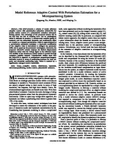
Fig. 4. Inverted Pendulum on a Cart used and then adaptively updated so that stability is assured. These parameters may not converge to their actual values, as discussed earlier. A failure is simulated, wherein the force on the cart freezes to a constant value that may or may not be zero. The controller is not supplied with the time of failure and the mathematical formulation of the controller does not change before and after the failure. Let M be the mass of the cart and m be the mass of the pendulum. I denotes the moment of inertia of the pendulum about its end. The system has two controls, the force on the cart (F ) and the torque on the pendulum (T ) The mathematical model for the inverted pendulum is:        ¨ I + ml mlcosθ   θ   mglsinθ  0 1 F    +   =   T 1 0 mlsinθθ˙2 x¨ mlcosθ M + m 

2

(2.51)

23

The model is of the form M (q, q)¨ ˙ q = G(q, q) ˙ + Cu The simulation is done with the following parameters listed in Tables I and II Table I. Variation in the Parameters for the Inverted Pendulum on a Cart Sr No.

Parameter

Actual Value

Guessed values

1.

Mass of the Cart

5 kg

6 kg

2.

Mass of the Pendulum

1 kg

0.5 kg

3.

Length of the Pendulum

5m

8m

Table II. The Error in the Initial Conditions for the Inverted Pendulum on a Cart Sr No.

States

Actual Values

Reference values

1.

Angular Position

87 degrees

67 degrees

2.

Angular Velocity

0 deg/sec

0 deg/sec

Simulation of failure: At time t=3 sec, the actuator corresponding to the force on the cart fails and the force attains a constant value of 10 N. Simulation results for model inversion with and without adaptation are presented in Figures 5, 6, 7, 8, 9 and 10. Consider Figure 5. At time equals zero, both the adaptive and the non-adaptive trajectories start from the same point, but away from the reference. As expected, Figure 5 shows that the controller with adaptation is able to effectively track the reference trajectory in spite of the actuator failure. The non-adaptive trajectory reaches steady state, but does not converge to the actual

24

Angle (deg)

100 Reference States with adaptive model inversion States with non−adaptive model inversion

50

0

Angular Velocity (deg/sec)

−50 0

5

10

5

10

15

20

25

15

20

25

20 0 −20 −40 −60 −80 0

Time (sec)

Fig. 5. Time Histories of Position and Velocity States for the Inverted Pendulum on a Cart The states that are not tracked Position of the cart (m)

500 States with adaptive model inversion States with non−adaptive model inversion

400 300 200 100

Velocity of the cart (m/sec)

0 0

5

10

5

10

15

20

25

15

20

25

40 30 20 10 0 0

Time (sec)

Fig. 6. Time Histories of Position and Velocity States for the Cart, that are Not Tracked

25

reference. This seems to be contrary to physical intuition at first thought. The feedback shows a tracking error, hence a control effort is generated. Since the model used for dynamic inversion is wrong intentionally to simulate improper modelling, the control does not drive the system to the desired equilibrium point, but stabilizes it at a different condition. Figure 6 shows that the cart continues to move with linearly increasing velocity. At a first glance, this seems to be contrary to the stability analysis done earlier, which proved that the trajectories are bounded and asymptotically converge to the reference. For this simulation the system model had 2 variables, the position of the cart (x) and the angular orientation of pendulum (θ). The only state that is tracked by the control is θ. Whenever only a subspace of the entire state space is tracked the stability of the internal dynamics has to be assured. The position of the cart cannot be ensured to stay within limits by just tracking the position of the pendulum. Hence the proposition of controlling the system by tracking only the pendulum was wrong in the first place. So the conclusion is that either the whole state space has to be tracked or the the stability of the internal dynamics has to be ensured if only some of the states are tracked. It is observed that the trajectories of the system as well as the controls are smooth. Thus it can be seen that the adaptive controller is able to recover from the failure with reasonable amount of control effort. Figure 7 shows that the adaptive controller effectively uses the control torque while the force control fails at t equals seconds and remains constant at 10 N. Since the force is constantly accelerating the cart, a nonzero torque is required to stabilize the pendulum in the vertical position. Figures 8, 9, and 10 show the convergence of the

26

U calc(adaptive) U calc(non−adaptive) U applied

Controls 20

Force (N)

10 0 −10 −20 0

5

10

15

20

25

15

20

25

Time (sec) 50

Torque (Nm)

0 −50 −100 −150 −200 0

5

10

Fig. 7. Time Histories of the Control for the Inverted Pendulum on a Cart 1.25 1.2 1.15 1.1

C

1.05 1 0.95 0.9 0.85 0.8 0

5

10

15

20

25

Time (sec)

Fig. 8. Update of the C Matrix for the Inverted Pendulum on a Cart

27

1.1

0.4 0.3 0.2

D12

D11

1 0.9

0.1 0.8

10

20

30

−0.1 0

0.6

1

0.4

0.8 D22

D21

0.7 0

0

0.2 0 −0.2 0

10

20

30

10 20 Time(sec)

30

0.6 0.4

10 20 Time (sec)

30

0.2 0

Fig. 9. Update of the D Matrix for the Inverted Pendulum on a Cart 0.02

E1

0.01 0 −0.01 −0.02 0

5

10

5

10

15

20

25

15

20

25

0.03 0.02

E2

0.01 0 −0.01 −0.02 −0.03 0

Time (sec)

Fig. 10. Update of the E Vector for the Inverted Pendulum on a Cart

28

Fig. 11. Definition of the Inertial and Body Axis system gains Ca , D, and E. The derivatives of the update parameters are functions of the tracking error, so the update parameters stop updating as soon as the tracking error goes to zero. H. Nonlinear Six-Degree-of-Freedom Simulation of an F-16 type aircraft with Thrust Vectoring 1. Definition of Variables and Development of a Non-Linear Mathematical Model of the F-16 type Aircraft The general equations of motion of an aircraft are derived for the body axis fixed to the airplane, with the origin at the center of gravity. The orientation and position

29

Fig. 12. Definition of Angle of Attack, α and Side-Slip, β of the airplane is defined in terms of an inertial reference frame fixed to the earth. (See Figure 11). Let dx, dy and dz denote the position of the aircraft along the X, Y and Z axes respectively. The angular orientation of the aircraft can be described by a 3-2-1 rotation sequence through the euler angles ψ, θ and φ, respectively. The angleof-attack and the side-slip angle can be defined in terms of the velocity components as w α = tan−1 ( ) u v β = sin−1 ( ) Vres

(2.52) (2.53)

where Vres is the resultant velocity. (See Figure 12). The variables that com-

30

pletely define the state-space for this aircraft model are the position level vector: · σ =

¸T

φ θ ψ dx dy dz

(2.54)

and the velocity level vector: · ω =

¸T (2.55)

p q r u v w

Following the earlier discussion, it is clear that the number of controls must be greater than the number of velocity level states. So there are eight controls on the hypothetical F-16 type aircraft: right horizontal tail, left horizontal tail, right aileron, left aileron, rudder, and additional three controls for thrust vectoring: thrust along the X, Y , and the Z axes. With a total of eight controls the control algorithm can tolerate a maximum of two control failures, both of which may fail at arbitrary times. Defining Sθ = sin(θ), Cθ = cos(θ), etc. The structured model with separate kinematic and dynamic parts can be written as 1. Kinematic Part: ·

¸T ˙ dy ˙ dz ˙ = φ˙ θ˙ ψ˙ dx  Cθ Cψ Sφ Sθ Cψ − Cφ Sψ Cφ Sθ Cψ − Sφ Sψ  C S S S S − C C C S S − S C φ θ ψ φ ψ φ θ ψ φ ψ  θ ψ   Sφ Cθ Cφ Cθ  −Sθ    0 0 0    0 0 0   0 0 0

0 0 0 1 0 0

(2.56)   0 0  p     0 0   q     0 0 r       Sφ tan(θ) Cφ tanθ  u     Cφ −Sφ   v    w Sφ secθ Cφ secθ

31

which is in the form of the model, Equation 2.8 σ˙ = J(σ)ω     p u      and linear velocity V =  v . 2. Dynamic Part: Let, angular velocity ω=  q         r w with I the moment of Inertia of the aircraft about the body axes and m the mass. The inertia matrix is 



Ixx Ixy Ixz     I= I I I  yx yy yz    Izx Izy Izz

(2.57)

From Euler’s rigid body equations, 





 L      −1   ω˙ = I M  − ω e Iω      N    X − mgSθ    ˙ = 1 Y + mgC S  V θ φ m   Z + mgCθ Cφ

(2.58)

(2.59)

where ω e V is the matrix representation of the cross-product between vector ω and vector V. 



 0 −r −q    ω e =  0 −p  r   −q p 0

(2.60)

32

The external moments and forces have contributions due to the aircraft wing and the fuselage that are dependent on the angle of attack and the sideslip angle; and the controls. Consider the total external pitching moment acting on the aircraft     1 2  2 ρV S(Cmmβ β + Cmmp p + Cmmr r) Cmmcont u M =  +  part1(unf orced) part2

(2.61)

where 12 ρV2 S is the dynamic pressure. Cmmβ , Cmmp , Cmmr r are the corresponding stability coefficients. Cmmconst is a row vector. The ith element of this vector represents the contribution to the pitching moment due to unit deflection of the ith control.

Since external moment and force contributions in part one of Equation 2.61play a role in the unforced dynamic behavior they form a part of the A matrix, while the external force and moment contributions in part two of Equation 2.61 form a part of the B matrix.

The dynamic part of the equation of motion can now be written as           L           Cucont   M  −ω e Iω  I −1            C     mmcont           N     unf orced   Cnncont   ω˙   u    +  =         ˙   Cxcont   V          −mgSθ      X         Cycont        1   −ω  m   e V  + mgC S Y θ φ               Czcont        Z mgCθ Cφ  unf orced

(2.62)

33

which has the same form as Equation 2.9 ω˙ = A(σ, ω) + B(σ, ω)uapp as desired 2.

Example # 2: Steady Level 1g Flight

Table III. The Reference States for Steady Level Flight φ = dy = dz = p = q = r = β = v = 0

ψ = constant

θ=α

dx = Vres t where t = time

u = Vres cosα

Vres = constant

w = Vres sinα

Example 2 tries to simulate steady level flight of the aircraft at 0.8 Mach and at an altitude of 50,000 ft. The aircraft is trimmed at angle of attack equal to 3 degrees. The simulation is done with parametric errors in the vector A and the B matrix, initial error conditions, and the right aileron fails at time equal to five seconds and settles down at a constant value of two degrees. Due to this failure the aircraft should start rolling rapidly. The adaptive controller is expected to adjust its parameters so that it compensates for this failure and provides a restoring rolling moment by using differential horizontal tail. The initial reference states are contained in Table III Figure 13 shows the angular states of the aircraft. Due to the failure of the right aileron the aircraft starts rolling rapidly. In the case with the non-adaptive controller the states of the system diverge. The linear states also diverge as seen in Figure 14 which shows that the non-adaptive controller is not able to handle the actuator

34

Adaptive Reference Non−Adaptive

4

2 p (deg/sec)

φ (deg)

1000 500 0 −500 0

5

q (deg/sec)

θ (deg)

2

5

5

10

5

10

0 −20 −40 0

10

50 r (deg/sec)

2 ψ (deg)

0

20

3

1 0 −1 0

1

−1 0

10

4

1 0

x 10

5 Time (sec)

10

0

−50 0

5 Time (sec)

10

Fig. 13. Time Histories of the Angular States of the Aircraft in Steady Level Flight

35

775 u (ft/sec)

dx (ft)

10000

5000

0 0

5

774 773 772 0

10

0

5

10

−20 0

5

10

60 w (ft/sec)

dz (ft)

10

0

0.2

0

−0.2 0

5

20 v (ft/sec)

dy (ft)

0.5

−0.5 0

Adaptive Reference Non−Adaptive

5 Time (sec)

10

40 20 0 0

5 Time (sec)

10

Fig. 14. Time Histories of the Linear States of the Aircraft in Steady Level Flight

36

Adaptive Reference

4

6

8

10

12

3

0.1

0

2

4

6

8

10

12

0

−0.1 0 10000

2

4

6 8 Time (sec)

10

12

5000 8

10

12

4

6

8

10

−5

0

2

4

6 8 Time (sec)

10

12

4

6

8

10

12

−1 0 1

2

4

6

8

10

12

2

4

6 8 Time (sec)

10

12

2

4

6

8

10

12

2

4

6

8

10

12

2

4

6 8 Time (sec)

10

12

0

773.6 773.4 0 1

12

0

2

0

−1 0 773.8

v (ft/sec)

6

0 −2 −4 0x 10 2 5

dz (ft)

4

−10 0 1

w (ft/sec)

dy (ft)

0 −3 0x 10 2 2

0

r (deg/sec)

2.8 ψ (deg)

2

u (ft/sec)

θ (deg)

−1 0 3.2

dx(ft)

p (deg/sec)

0

10

q (deg/sec)

φ (deg)

1

0 −1 0 42 41 40

0

Fig. 15. Time Histories of the States of the Aircraft with Adaptive Control in Steady Level Flight

37

Adaptive

Non Adaptive rHT

100

0 10

−100 100 0

12 lHT

8

2

4

6

8

10

4

6

8

10

−20 10 0

2

4

6

8

10

−10 1710 0

2

4

6

8

10

12

1700 4

6

8

10

12

0 −50 20 0

2

4

6

8

10

12

0 −20

0

2

4

6

Time (sec)

8

10

12

5

6

7

1

2

3

4

5

6

7

1

2

3

4

5

6

7

1

2

3

4

5

6

7

0 x 104 1 20

2

3

4

5

6

7

2

3

4

5

6

7

1

2

3

4

5

6

7

1

2

3

4

5

6

7

0

0

ThrustY

2

ThrustZ

ThrustZ

ThrustY

1690 50 0

4

−100 100 0

12

0

3

−100 100 0

12

0

2

−100 100 0

12

lTEF

2

1

0

rTEF

rTEF lTEF

6

0 −20 20 0

rudder

4

0 −20 20 0

ThrustX

2

rudder

lHT

−20 20 0

0

ThrustX

rHT

20

50

0 −2 x 104 1 20 0

−2 2000 0 0

−2000

0

Time (sec)

All control surface deflections are in degrees and all thrusts are in lbs

Fig. 16. Time Histories of the Controls of the Aircraft in Steady Level Flight

38

failure and hence the states diverge. Figure 15 shows the states of the aircraft with the adaptive controller. The departure in the states from the reference before failure (when time is less than five seconds) is due to the initial errors and the parametric error in the system matrices, but the states settle down to their reference values by time equal to five seconds. All the states show perturbations at failure (when time is equal to five seconds), but the controller adapts to this failure and the states settle down to their reference values. Figure 16 shows the controls. The controls generated by the adaptive controller are smooth and within reasonable limits. The recovery from failure and the performance shown is achieved with reasonable control deflection limits. The control rates (not shown) are also within reasonable limits. The update parameters (not shown) stop updating as soon as the tracking error goes to zero, similar to the inverted pendulum on a cart example shown earlier. 3. Example # 3: Steady Level Turn Example 3 tries to simulate steady level turn of the aircraft at 0.8 Mach and at an altitude of 50,000 ft. The aircraft is turning at a constant rate of 3 degrees/second and is banked at an angle of 52.4 degrees. The trim angle of attack is 14 degrees. In Table IV. The Reference States for Steady Level Turn α = constant

p = −sinθψ˙

˙ ψ = ψt

q = cosθsinφψ˙

θ = constant

r = cosθcosφφ˙

φ = constant

u = Vres cosα

dx = Vres t

w = Vres sinα

dy = dx = β = v = 0

Vres = constant

39

this simulation, the right aileron fails at time equal to five seconds and settles down to a value of one degree. There is no initial condition error and no uncertainties in the system parameters. The reference states are shown in the Table IV The reference states for steady level turn are a constant turn rate, ψ˙ and bank angle,

Fig. 17. Steady Level Turn ˙

bank = tan−1 ( ψV ). For a steady level turn, the transformation from the inertial axis g to the body axis is a 3-1-2 Euler Angle rotation through ψ, bank and α respectively. This 3-1-2 rotation is converted to a 3-2-1 rotation to obtain ψ, θ and φ. Figures 18 and 19 show that the states of the aircraft with the non-adaptive controller exhibit perfect tracking with respect to the reference until failure, but diverge rapidly afterwards. In Figure 20 all the states show perturbations at failure (when time is equal to five seconds), but the controller adapts to this failure and the

40

states settle down to their reference values. The adaptive learning parameters remain constant before failure as there are no initial errors or errors in system parameters, but they update after failure and settle down to constant values which are different from the initial values. Also, Figure 21 shows that the controls generated by the adaptive controller are smooth and within limits. Also the control rates (not shown) are within limits. So the adaptive controller recovers from the failure with reasonable control effort.

60

500

40

0

p (deg/sec)

φ (deg)

41

20 0 −20

0

5

10

15

−1000 −1500

8 7

0

5

10

10

15

0

5

10

15

0

5

10

15

−10

20 r (deg/sec)

ψ (deg)

5

0

−20

15

60 40 20 0

0

10 q (deg/sec)

θ (deg)

9

6

Adaptive Reference Non−Adaptive

−500

0

5

10 Time (sec)

15

0 −20 −40

Time (sec)

Fig. 18. Time Histories of the Angular States of the Aircraft Performing a Steady Level Turn

42

790

10000

u (ft/sec)

dx (ft)

15000

5000 0

0

5

10

4000 2000

5

10

15

0

5

10

15

0

5

10

15

−50 −100

0

5

10

15

−150 200 w (ft/sec)

0.2 dz (ft)

0

0

0.4

0 −0.2 −0.4

780

50 v (ft/sec)

dy (ft)

6000

0

785

775

15

Adaptive Reference Non−Adaptive

0

5

10 Time (sec)

15

150 100 50

Time (sec)

Fig. 19. Time Histories of the Linear States of the Aircraft Performing a Steady Level Turn

43

5

10

15

8.5

8.4 0 100

5

10

15

50 5

10

15 u (ft/sec)

Time (sec)

1 5

10

15

dy (ft)

0 0 5000

5

10

−5

0

5

10 Time (sec)

15

10

15

5

10

15

10

15

5

10

15

5

10

15

10

15

2.5 2 0 3 2

775.5 0 10

15

0

5

5 Time (sec)

776

w (ft/sec)

dz (ft)

0 −3 0x 10 5

−10 0 3

1 0 776.5

v (ft/sec)

dx(ft)

0 4 0x 10 2

0

r (deg/sec)

θ (deg)

50 0 8.6

ψ (deg)

p (deg/sec)

52

10

q (deg/sec)

φ (deg)

54

Adaptive Reference

0 −10 0 195 194 193

0

5 Time (sec)

Fig. 20. Time Histories of the States of the Aircraft with Adaptive Control, Performing a Steady Level Turn

44

Adaptive

Non Adaptive rHT

100

−20

lHT

5

10

5

10

15

0 5

10

15

1500

ThrustY

1000 100 0

5

10

15

50 0 100 0

0

5

10

5

10

Time (sec)

15

15

2

3

4

5

1

2

3

4

5

1

2

3

4

5

1

2

3

4

5

1

2

3

4

5

1

2

3

4

5

1

2

3

4

5

1

2

3

4

5

50 0 00

15 lTEF

−50 10 0

−10 2000 0

ThrustZ

−100 100 0

15

1

−50

rTEF

10

rudder

rTEF lTEF

5

0

50

0 −100 00

15

0 −50 50 0

rudder

10

−20 −40 50 0

ThrustX

5

ThrustX

lHT

−40 00

ThrustZ (lb) ThrustY

rHT

0

−50 −100 100 0 0

−100 10000 0 5000 0 2000 0 0 −2000 1000 0 0 −1000

0

Time (sec)

All control surface deflections are in degrees and all thrusts are in lb

Fig. 21. Time Histories of the Controls of the Aircraft Performing a Steady Level Turn

45

CHAPTER III

MODIFIED REFERENCE STRUCTURED ADAPTIVE MODEL INVERSION CONTROL WITH ACTUATOR SATURATION CONSTRAINTS A. Introduction This chapter discusses the problems that are faced in adaptive systems due to saturation. Techniques to avoid saturation are discussed and the concept of modifying the reference trajectory to avoid saturation is suggested. A mathematical formulation is derived and an example is presented for the problem of an inverted pendulum. This method is compared with the strategy of stopping adaptation on saturation, and continuing adaptation on saturation, while continuing to track the original reference in both the cases. B. Control Saturation Limits and Problems Introduced in Adaptive Systems due to Saturation Traditional adaptive control usually assumes full authority control, and lacks an adequate theoretical treatment for control in the presence of actuator saturation limits. By full authority it is implied that no constraints are placed on the control effort or on the rate with which the control can change. Physical actuators that are used in actual dynamic systems are subjected to position and rate constraints. For example, the flaps on an aircraft have a limit on the maximum angular deviation that they can have from the zero position. Also, the flaps cannot move from one position to another, faster than a particular angular velocity. Because of these limitations the actual control applied is not the same as the calculated control, which can cause tracking errors and even divergence.

46

Saturation is more critical for adaptive systems than non adaptive systems. In SAMI, the adaptation is based on the tracking error between the reference and the actual plant. Assuming that the dynamics are modelled perfectly and only parametric uncertainties exist in the system, the tracking error has contributions due to the initial condition error, parametric uncertainties, and saturation. The adaptation scheme aims to adapt only the uncertain parameters in the mathematical model of the plant. Thus, the error driving the adaptation scheme should only be the error due to the uncertain parameters, and not include the tracking error due to saturation. Including the error component due to saturation will cause incorrect adaptation. Attempts to handle saturation in adaptive systems usually follows one of the two approaches: • Reduce the adaptation rate in the presence of saturation, or completely stop adaptation when the control is saturated [11]. This stops the incorrect adaptation, but adaptation may be critical when the input is saturated. For instance, consider a case where the parametric uncertainty is high and the control saturates because of these uncertainties. The system may diverge unless the uncertainties are corrected, and may not recover from saturation at all. • If the input is saturated due to an aggressive reference trajectory, the reference command is adjusted so that the input does not saturate. In this thesis an adaptive control methodology is developed which follows the latter approach. After separating the system into structured kinematic and dynamic parts, it is noticed that the control directly affects the acceleration. The difference between the calculated and the applied control effort due to saturation results in a lack of acceleration produced in the plant, as compared to the demanded reference

47

acceleration. This is called the hedging signal [16][17] [18]. If the hedge is removed from the reference, the resulting modified reference can be tracked within saturation limits . The tracking error seen will be due only to the initial error and the parametric uncertainty, hence the controller will adapt correctly. The SAMI formulation will always remain unsaturated because of the modified reference, but the focus now shifts to the stability of the reference model as the the reference model now gets dynamically coupled with the plant and the adaptive law. The hedge signal now acts as an exogenous input to the reference model. But, the reference model is a hypothetical mathematical model selected by the designer and therefore is free from the input rate and position saturation constraints. Hence, ensuring stability in the presence of bounded disturbances is simplified. C. Mathematical Formulation Consider the mathematical model of the system as follows M (q, q)¨ ˙ q = G(q, q) ˙ + Cuapp q ¨ = M −1 G + M −1 Cuapp

(3.1) (3.2)

where • q ∈ Rn = vector of generalized coordinates • M (q, q) ˙ ∈ Rn×n = mass matrix • G(q, q) ˙ ∈ Rn = vector of nonlinear functions of the states used to describe the unforced dynamic behavior • C ∈ Rn×m = control influence matrix

48

• u ∈ Rm = vector of the control inputs. (m should be at least equal to n). The dynamics of the system are assumed to be modelled accurately, and only structured parametric uncertainties exist in the model. This second-order differential equation can be split up into kinematic and dynamic parts as σ˙ = ω

(3.3)

ω˙ = A(σ, ω) + B(σ, ω)uapp

(3.4)

where • σ∈ Rn = q = vector of position level coordinates • ω∈ Rn = q˙ = vector of velocity level coordinates • A(σ,ω) = M −1 G • B(σ,ω) = M −1 C

Consider a linear reference model        I  σr   0  σ˙ r   0   =     +   ur ω˙ r Ar1 Ar2 ωr B

(3.5)

Considering a more general case the kinematic equation can be written as σ˙ = Jω where J ∈ Rn×n = nonlinear transformation relating σ˙ and ω. The linear reference will have a constant in the place of I, in Equation 3.5.

49

Let the error in the position and the velocity level states be s and x respectively, s = σ − σr

(3.6)

x = ω − ωr

(3.7)

The control appears only in the velocity level equation, and hence the corresponding velocity level error. The control affects the position through the integration of Equation 3.4 via the coupling seen in Equation 3.3 x˙ = ω˙ − ω˙ r

(3.8)

x˙ = A + Buapp − ω˙ r

(3.9)

However, the error between the reference and the plant must go to zero. Hence the dynamics prescribed for x are x˙ = Ah x + φ

(3.10)

where Ah = Hurwitz matrix, i.e. all eigenvalues lie in the open left half plane so that the velocity error dynamics are stable. Ah can be selected arbitrarily, but a proper choice can specify how fast the velocity error stabilizes. φ = forcing function on the velocity error dynamics, which helps in achieving the tracking objective. This is discussed in detail later. Adding and subtracting Ah x + φ on the right hand side x˙ = Ah x + φ + A + Buapp − (ω˙ r + Ah x + φ)

(3.11)

50

Since the quantity in the parenthesis is known, let ψ , ω˙ r + Ah x + φ

(3.12)

Such that x˙ = Ah x + φ + A + Buapp − ψ

(3.13)

Using dynamic inversion to solve for the control, ucal = B −1 (ψ − A)

(3.14)

But the system parameters A and B are not known accurately, hence best guesses for A and B called Aest and Best will be used. Let the calculated control be, ucal = (Cb Best )−1 (ψ − Ca Aest )

(3.15)

Where Ca and Cb are the adaptive learning matrices which will be updated online thereby ensuring stability and performance of the system. There exist matrices Ca∗ and Cb∗ such that Ca∗ × Aest = A

(3.16)

Cb∗ × Best = B

(3.17)

But the control has saturation limits. So, the applied control is      ucal if |ucal | ≤ umax  uapp =  umax sign(ucal ) if |ucal | > umax  

(3.18)

Now, let δ be the difference between the calculated control and the applied control δ = ucal − uapp

(3.19)

51

From Equation 3.15 and Equation 3.19, uapp = (Cb Best )−1 (ψ − Ca Aest ) − δ

(3.20)

ψ = Ca Aest + Cb Best uapp + Cb Best δ

(3.21)

So that

Substituting in Equation 3.13 results in x˙ = Ah x + φ + Ca∗ Aest + Cb∗ Best uapp − Ca Aest − Cb Best uapp − Cb Best δ(3.22) Defining the tilde quantities as the error between the actual value of the update parameter and the currently learned value, ea , Ca∗ − Ca C

(3.23)

eb , C ∗ − Cb C b

(3.24)

Equation 3.22 now becomes ea Aest + C eb Best uapp − Cb Best δ x˙ = Ah x + φ + C

(3.25)

Cb Best δ represents the acceleration that could not be supplied because of the saturation limit, and is termed the hedging signal. Subtracting this hedging signal from the reference trajectory so that the resulting ucal obtained is within saturation limits, results in ea Aest + C eb Best uapp ω˙ − (ω˙ r − Cb Best δ) = Ah x + φ + C

(3.26)

ω˙ r (modif ied) = (ω˙ r − Cb Best δ)

(3.27)

52

Note that Cb Best δ acts as a disturbance on the model reference. The modified reference is now: 





σ˙ r   0   =  ω˙ r Ar1





    I   σr   0   0     +   ur −  δ Ar2 ωr B Cb Best

(3.28)

It is assumed that although the control saturates initially while following the reference trajectory, after some point of time, the control demanded to track the reference will be within saturation limits. This ensures that |δ| goes to zero after some time. R∞ Hence, δ is a bounded energy type disturbance, i.e. 0 δ 2 dt is bounded. Since the reference plant is linear and specified by the designer, a controller can be designed so that the modified reference eventually converges with the original reference trajectory.

The modified acceleration tracking error is ea Aest + C eb Best uapp x˙ = Ah x + φ + C

(3.29)

Let the total tracking error be defined as y , s˙ + λs

(3.30)

where λ ∈ Rn×n is a positive definite matrix. As t → ∞, if y is driven to zero, it is ensured that s → 0 and s˙ → 0. y˙ = x˙ + λx

(3.31)

ea Aest + C eb Best uapp y˙ = (Ah x + φ + λx) + C

(3.32)

Substituting for x, ˙

53

ea and C eb are not. For the tracking The quantity in the parenthesis is known, while C error to stabilize, the following dynamics are prescribed to the quantities within the parenthesis. The uncertain quantities will be taken care of with a Lyapunov analysis done later. Thus y˙ = Ah y Ah y = (Ah x + φ + λx)

(3.33) (3.34)

which gives the forcing function φ: φ = λ(Ah s − x)

(3.35)

Finally, ea Aest + C eb Best uapp y˙ = Ah y + C

(3.36)

Now consider the error departure function as the candidate Lyapunov function. If P, W1 , W2 are positive definite matrices, eT W1 C ea + C e T W2 C eb ) V = yT P y + T r(C a b

(3.37)

Taking the derivative of the Lyapunov function V˙

e T W1 C e˙ a + C e T W2 C e˙ b ) = yT P y˙ + y˙ T P y + 2T r(C a b

V˙

eT e T P y + uT B T C = yT P Ah y + yT ATh P y2T r(ATest C app est b P y) a e˙ b ) e˙ a + C ebT W2 C eaT W1 C +2T r(C

(3.38)

(3.39)

P is selected such that P Ah + ATh P = −Q, where Q is a positive definite matrix. Existence of P and Q to satisfy the above relation is guaranteed as Ah is Hurwitz.

54

Also using the identity: If A and B are row and column matrices respectively, then AB = T r(BA): V˙

eT (P yAT + W1 C e˙a ) = −yT Qy + 2T r(C a est T ebT (P yuTapp Best e˙ b )) +2T r(C + W2 C

(3.40)

ea = C ∗ −Ca cannot be calculated since the values of the actual parameters, Note that C a such as Ca∗ , are not known. Therefore the coefficient of Ca∗ must go to zero. Retaining only the negative definite part, −yT Qy, and setting all other terms to zero, e˙ a = −W −1 (P yAT ) C 1 est

(3.41)

C˙ a∗ − C˙ a = −W1−1 (P yATest )

(3.42)

However, Ca∗ is assumed to be constant, so that C˙ a = W1−1 (P yATest )

(3.43)

T C˙ b = W2−1 (P yuTapp Best )

(3.44)

Similarly,

These are the update equations for the various adaptive learning parameters. The stability analysis is similar to the stability analysis done in Chapter II, section F. Figure 22 shows the schematic diagram of a modified reference structured adaptive model inversion controller. D. Numerical Example # 1 : Control of an Inverted Pendulum The examples will compare the modified reference control strategy, with the strategy of continuing adaptation based on the original reference, and the strategy of

55

Fig. 22. Schematic diagram of a Modified Reference Structured Adaptive model Inversion Controller with Actuator Saturation Constraints

56

stopping adaptation on saturation to prevent incorrect adaptation. In the first example, comparison between two cases is presented 1. Adaptation is continued even when the input saturates. The original reference trajectory is not modified. 2. Adaptation is continued throughout and the hedge signal is subtracted from the reference to prevent saturation.

Fig. 23. Inverted Pendulum

Consider an inverted pendulum as shown in Figure 23 with the following parameters. Let the mass of the pendulum be m, the length be l and the moment of inertia, I=

ml2 . 3

The system has one control: torque on the pendulum = T . Angle made by

the pendulum with the vertical is denoted by θ. Note that θ is the angular position, therefore θ˙ is the angular velocity. The mathematical model for the pendulum is l I θ¨ = mg sin(θ) + T 2 The simulation is done with the parameters listed in tables V and VI

(3.45)

57

Table V. Variation in the Parameters for the Inverted Pendulum (Example 1) Sr No.

Parameter

Actual Value

Guessed values

1.

Mass of the Pendulum

2 kg

2.5 kg

2.

Length of the Pendulum

1m

0.8 m

3.

Acceleration due to gravity

9.8 kg m/s

9.5 kg m/s

Table VI. The Error in the Initial Conditions for the Inverted Pendulum (Example 1). Sr No.

States

Actual Values

Reference values

1.

Angular Position

83 degrees

80 degrees

2.

Angular Velocity

13 deg/sec

10 deg/sec

The objective is to come to rest at the vertical position. Figure 24 shows the evolution of the position and the velocity level states. Until the command is saturated, the system follows the same state with or without the hedge since the control applied in both the cases is umax sign(ucal ). Although the trajectories are the same, the learning parameters are being updated due to different error signals in both cases. Without hedging the error is the sum of the errors due to initial error conditions, uncertainties in the system parameters, and also errors due to saturation. While with hedging the error due to saturation is zero as the reference is modified to avoid saturation. Thus the adaptation is accurate. Also, note the modified trajectory is quite different from the original desired reference, because of saturation. After the system comes out of saturation (time ≈ 4.5 seconds)the modified trajectory begins converging to the original reference. The control with the hedge shows better tracking than without the hedge, because of correct adaptation in

58

100 Tracking without hedge Original reference Tracking with hedge Modified reference

position(deg)

80 60 40 20 0 −20 −40

0

1

2

3

4

0

1

2

3

4

5

6

7

8

9

10

5

6

7

8

9

10

velocity (deg/sec)

300 200 100 0 −100 −200 −300

Time (sec)

Fig. 24. Time Histories of Position and Velocity States for the Inverted Pendulum (Example 1) 150 Ucal without hedge Uapp without hedge Ucal with hedge Uapp with hedge

100

Torque (N.m)

50

0

−50

−100

−150

−200

0

1

2

3

4

5

6

7

8

9

10

Time (sec)

Fig. 25. Time Histories of Controls for the Inverted Pendulum (Example 1)

59

Without hedge

With hedge

200

60 59.5

Ca

59

Ca

150

100

58.5 58 57.5

50

0

2

4

6

8

57

10

50

57.2

40

57

2

0

2

4

6

8

10

4

6

8

10

Cb

57.4

Cb

60

0

30

56.8

20

56.6

10

0

2

4

6

8

10

56.4

Time (sec)

Time (sec)

Fig. 26. Update of the Adaptive Parameters for the Inverted Pendulum (Example 1) the former case. Since the modelling errors and initial errors are small, the tracking with the hedge closely follows the modified reference. Figure 25 shows that the control required in the case with the hedge is smaller in magnitude than control without the hedge. Figure 26 shows that the adaptive parameters converge to different values for both cases. Also, the change in the adaptive parameters is greater in the control strategy without the hedge. E. Numerical Example # 2 : Control of an Inverted Pendulum In the second example, comparison between the following two cases is presented 1. Stopping adaptation on saturation, but still continuing to track the original

60

reference. 2. Adaptation is continued throughout and the hedge signal is subtracted from the reference to prevent saturation. The simulation is done with the parameters listed in tables VII and VIII Table VII. Variation in the Parameters for the Inverted Pendulum (Example 2) Sr No.

Parameter

Actual Value

Guessed values

1.

Mass of the Pendulum

2 kg

3 kg

2.

Length of the Pendulum

1m

0.8 m

3.

Acceleration due to gravity

9.8 kg m/s

9.8 kg m/s

Table VIII. The Error in the Initial Conditions for the Inverted Pendulum (Example 2). Sr No.

States

Actual Values

Reference values

1.

Angular Position

90 degrees

90 degrees

2.

Angular Velocity

350 deg/sec

350 deg/sec

The objective is to come to rest at the vertical position. In Figure 27, control strategy 1 shows divergence. This is because the control becomes saturated very soon due to the uncertain parameters, and since adaptation is stopped it does not recover. Control strategy 2 shows that, with the adaptation and the modified reference, the plant is able to recover and converge to the original reference. Figure 28 shows that the control in the case without the hedge diverges.

61

Without Hedge

4

1

x 10

With Hedge 200

position(deg)

position(deg)

0 −1 −2 −3 −4

100 50 0

−5 −6

0

2

4

6

8

−50

10

0

2

0

2

4

6

8

10

4

6

8

10

400

velocity (deg/sec)

velocity (deg/sec)

5000

0

−5000

−10000

−15000

Original Reference Trajectory followed Modified reference

150

0

2

4

6

8

300 200 100 0 −100 −200

10

Time (sec)

Time (sec)

Fig. 27. Time Histories of Position and Velocity States for the Inverted Pendulum (Example 2) Without hedge

7

Torque (N.m)

5

x 10

0

−5

−10

−15

0

1

2

3

4

5

6

7

8

9

10

9

10

With Hedge

Torque (N.m)

20 0 −20 −40 Ucal Uapp

−60 −80

0

1

2

3

4

5

6

7

8

Time (sec)

Fig. 28. Time Histories of Controls for the Inverted Pendulum (Example 2)

62

Without Hedge

With Hedge

64

55

62

50

Ca

60

Ca

66

60

45

58

40

56

0

2

4

6

8

35

10

60

0

2

0

2

4

6

8

10

4

6

8

10

70

50

65 60

30

Cb

Cb

40

20

55

10 50

0 −10

0

2

4

6

Time(sec)

8

10

45

Time(sec)

Fig. 29. Update of the Adaptive Parameters for the Inverted Pendulum (Example 2) Figure 29 shows the update of the adaptive parameters. Note that the parameters in the case without the hedge stop adapting after time ≈ 0.5 sec, because the control saturates.

63

CHAPTER IV

CONTROLLER TO HANDLE COMBINED ACTUATOR FAILURES AND ACTUATOR SATURATION Controllers to handle Actuator Failures and Actuator Saturation separately, have been developed in the previous chapters. If an actuator fails, the system may start to diverge, and to recover from this failure the remaining active controls may saturate. To handle these kind of situations, a controller to handle combined actuator failure and actuator saturation is developed. A nonlinear six-degree-of-freedom simulation of an aircraft with both actuator failure and actuator saturation is presented. A. Mathematical Formulation Consider the mathematical model of the system as follows σ˙ = J(σ)ω ˙

(4.1)

ω˙ = A(σ, ω) + B(σ, ω)uapp

(4.2)

where • σ∈ Rn = q = vector of position level coordinates • ω∈ Rn = q˙ = vector of velocity level coordinates • J ∈ Rn×n = nonlinear transformation relating σ˙ and ω

Substituting for ucal from the failure model (Equation 2.1) as uapp = Ducal + E ω˙ = A(σ, ω) + B(σ, ω)Ducal + B(σ, ω)E

(4.3)

64

Consider a linear reference model        σ˙ r   0 Jr0  σr   0    =     +   ur ω˙ r Ar1 Ar2 ωr B

(4.4)

where Jr0 is the value of Jr , where the system is linearized. Jr is the nonlinear transformation matrix relating σr and ωr . Let the error in the position and the velocity level states be s and x respectively s = σ − σr

(4.5)

x = ω − ωr

(4.6)

For the velocity error to converge we prescribe the following dynamics, x˙ = Ah x+ φ. Hence x˙ = Ah x + φ + A + BDucal + BE − ψ

(4.7)

where ψ , ω˙ r + Ah x + φ

(4.8)

Using dynamic inversion to solve for the control, ucal = pinv(BD)(ψ − A − BE)

(4.9)

ucal = pinv(Best D)(ψ − Ca Aest − Best E)

(4.10)

Let

where Aest and Best are the best estimated values of A and B respectively, and Ca is the adaptive learning parameter.

65

Using control hedging on saturation, the hedged control can be written as, uhed = pinv(Best D)(ψ − Ca Aest − Best E) − δ

(4.11)

So the derivative of the velocity error now becomes e − Best Dδ ea Aest + Best Du e cal + Best E x˙ = Ah x + φ + C

(4.12)

e ea Aest + Best Du e cal + Best E ω˙ − (ω˙ r − Best Dδ) = Ah x + φ + C

(4.13)

Therefore the modified reference now is ω˙ − (ω˙ r − Best Dδ)

(4.14)

The derivation proceeds from this point, on similar lines as the derivations in chapters II and III. B. A Nonlinear Six-Degree-of-Freedom Simulation of an F-16 type Aircraft with Simultaneous Actuator Failure and Actuator Saturation This example tries to simulate steady level flight of the aircraft at 0.8 Mach and at an altitude of 50,000 ft. The aircraft is trimmed at angle of attack equal to 3 degrees. The simulation is done with parametric errors in the vector A and the B matrix, initial error conditions, and the right aileron fails at time equal to five seconds and settles down at a constant value of negative one degree. Due to this failure the aircraft starts rolling rapidly. In an attempt to recover from this failure some of the remaining controls saturate. Now, if the adaptation is turned off during saturation, the system diverges. But by doing control hedging it is possible to continue adapting and recover from the failure, in spite of the saturation.

66

The first set of graphs (Figures 30-32) show the time histories for case where adaptation is stopped on saturation. From figure 32 it is seen that the controls saturate at time approximately equal to 6.5 seconds. All the angular and the linear states start diverging at this time as seen from figures 30 and 31 respectively. This is because the controls saturated due to the failure and if adaptation is stopped after failure the system cannot recover from the failure. The figures for Case 2 show the time histories of the states and the controls when the reference is modified by the hedging signal. The basic idea here is to modify an aggressive reference trajectory so that the resulting trajectory can be tracked within control limits. When the right aileron has failed and the aircraft is rolling rapidly large control deflections are needed to bring it back to horizontal position immediately. From Figure 33 it is seen that the hedging signal modifies the reference trajectory in such a way that the trajectory becomes less aggressive. Instead of returning to the horizontal position immediately, the reference trajectory demands that the aircraft return to the horizontal position smoothly. This is seen from the trajectory for the euler angle φ from Figure 33. Figure 34 shows that the linear states of the aircraft converge to the reference and Figure 35 shows that the controls are within bounds.

67

Angular States of the Aircraft

4

1 p (deg/sec)

φ (deg)

500 0 −500 −1000

0

2

4

3.5 q (deg/sec)

θ (deg)

2.5 2 0

2

4

2

4

6

0

2

4

6

0

2

0

50 r (deg/sec)

ψ (deg)

0

20

−20

6

2 0 −2 −4

Adaptive Reference

−1

40

3

1.5

0

−2

6

x 10

0

2

4 Time (sec)

6

0 −50 −100

4 Time (sec)

6

Fig. 30. Time Histories of the Angular States of the Aircraft in Steady Level Flight with Simultaneous Actuator Failure and Actuator Saturation (Case1)

68

774

4000

772

2000 0

dy (ft)

u (ft/sec)

6000

0

2

4

0.2

10

0

0

−0.2 −0.4

2

4

6

0

2

4

6

0

2

−10

0

2

4

−30

6

0.3

60

0.2

40

0.1 0 −0.1

0

−20

w (ft/sec)

dz (ft)

−0.6

Adaptive Reference

770 768

6

v (ft/sec)

dx (ft)

Linear States of the Aircraft

20 0

0

2

4 Time (sec)

6

−20

4 Time (sec)

6

Fig. 31. Time Histories of the Linear States of the Aircraft in Steady Level Flight with Simultaneous Actuator Failure and Actuator Saturation (Case 1)

69

rHT

20 0

lHT

−20 20 0

2

3

4

5

6

1

2

3

4

5

6

1

2

3

4

5

6

1

2

3

4

5

6

1

2

3

4

5

6

1

2

3

4

5

6

1

2

3

4

5

6

1

2

3

4

5

6

0

rTEF

−20 20 0 0

lTEF

−20 20 0 0 −20 20 0 0 −20 x 105 20 0 −2 x 104 50

ThrustY

ThrustX

rudder

1

0

ThrustZ

−5 x 104 10 0

−1

0

Time (sec) All control surface deflections are in degrees and all thrusts are in lbs

Fig. 32. Time Histories of the Controls of the Aircraft in Steady Level Flight with Simultaneous Actuator Failure and Actuator Saturation (Case 1)

70

1

10

0

5

p (deg/sec)

φ (deg)

Angular States of the Aircraft

−1 −2 −3

0

5

10

3.3 q (deg/sec)

θ (deg)

3.1 3 0

5

10

5

10

15

0

5

10

15

0

5

10

15

0

1 r (deg/sec)

0.1 ψ (deg)

0

0.5

−0.5

15

0.15

0.05 0 −0.05

−5

1

3.2

2.9

0

−10

15

Adaptive Reference

0

5

10 Time (sec)

15

0.5 0 −0.5

Time (sec)

Fig. 33. Time Histories of the Angular States of the Aircraft in Steady Level Flight with Simultaneous Actuator Failure and Actuator Saturation (Case 2)

71

Adaptive Reference

15000

773.6

10000

773.5

u (ft/sec)

dx (ft)

Linear States of the Aircraft

5000 0 2

0 −3 x 10

5

10

15

773.3

v (ft/sec)

−2 −4 −6 2

0 −4 x 10

5

10

10

15

0

5

10

15

0

5

10

15

0 −1

−3

15

44 w (ft/sec)

dz (ft)

5

−2

0 −2 −4 −6

0

1

0 dy (ft)

773.4

43 42 41

0

5

10 Time (sec)

15

40

Time (sec)

Fig. 34. Time Histories of the Linear States of the Aircraft in Steady Level Flight with Simultaneous Actuator Failure and Actuator Saturation (Case 2)

72

rHT

20 0

lHT

−20 20 0

rTEF lTEF rudder ThrustX

15

5

10

15

5

10

15

5

10

15

5

10

15

5

10

15

5

10

15

10

15

0 −20 20 0

ThrustY

10

0 −20 20 0

ThrustZ

5

0 −20 20 0 0

−20 1710 0 1700 1690 50 0 0 −50 50 0 0 −50

0

5

Time (sec) All angles are in degrees and all thrusts are in lbs

Fig. 35. Time Histories of the Controls of the Aircraft in Steady Level Flight with Simultaneous Actuator Failure and Actuator Saturation (Case 2)

73

CHAPTER V

CONCLUSIONS Model Reference Adaptive Control is a well developed methodology. The mathematical model of a system can be broken down into an exactly known kinematic part and an uncertain dynamic part. The adaptation is simplified by restricting the adaptation to the dynamic level equation. This leads to the development of Structured Model Reference Adaptive Control and Structured Adaptive Model Inversion Control. This thesis introduces the concept of adding a mathematical model of controller failure to the plant model, so that the above controllers can be made fault tolerant. It also incorporates into the SMRAC/SAMI framework, the idea of modifying the reference trajectory, to facilitate correct adaptation in the presence of saturation. This thesis derives and validates a Fault Tolerant Structured Adaptive Model Inversion Control Law and a Modified Reference Structured Adaptive Model Inversion Control Law to accommodate actuator position constraints. The control laws ensure global asymptotic stability of the tracking errors. However the adaptive learning parameters may not converge to the actual parameters within the duration of the maneuver.

Based on the preliminary results presented in the thesis, the following conclusions are made. For the Fault Tolerant Structured Adaptive Model Inversion Control Law: 1. The adaptive controller is able to achieve close tracking in presence of actuator failure, even though for the non-adaptive formulation, actuator failure may

74

result in loss of tracking or total instability as seen from the simulations. Thus the adaptive controller is able to recover from the failure while the non-adaptive controller is not. 2. This formulation can only handle those parametric uncertainties that are constant with respect to time or slowly time varying as compared to the rate of update of the adaptive learning parameters of the system. Therefore, the fault tolerant controller can handle actuator freezes, in which the control effort remains constant with respect to time. This constant value may or may not be zero. This is with the assumption that the system is controllable with the remaining active controls and the control effectiveness of the remaining controls is large enough to compensate for the lack of effort produced by the failed control and to counter the undesirable control produced when the actuator settles to an arbitrary value. For the Modified Reference Structured Adaptive Model Inversion Control Law: 1. The modified reference control methodology shows close tracking performance as compared to the strategy of tracking the original reference and the strategy of stopping the adaptation on saturation. In the test case shown, the strategy of modifying the reference shows close tracking even though the trajectory diverges for the strategy of stopping adaptation on saturation. 2. In the saturated condition, the performance with and without the hedge is essentially the same because the control applied is umax sign(ucal ) for both the cases. During saturation, the adaptation with the hedge is better, because the parameters are updated due to the correct error signal. So, when the plant comes out of saturation the performance is better due to the better adaptation.

75

CHAPTER VI

RECOMMENDATIONS AND FUTURE RESEARCH DIRECTIONS 1. Fault Tolerance to other types of failures: The research presented in this thesis can handle actuator freezes or partial loss of control effectiveness in the sense that the new control effectiveness can be obtained as a product of the the old control effectiveness and a constant. This was done by identifying a structure which modelled control application, uapplied = Ducalculated + E. Thus the task of identifying a control failure is just identifying the values of the D and the E parameters. Similarly a structure can be identified for any other type of failure, that can model the normal behavior and the failure just by the change of the value of a parameter. Thus fault tolerance for other types of failure can be investigated. 2. Actuator Rate Limiting: Physical actuators are not only limited by position limits but also by rate limits. This thesis focuses only on position constraints. This research should be extended to accommodate actuator rate constraints. 3. Pilot Induced Oscillations(PIO): PIOs may be defined as undesirable oscillations induced in the aircraft motions due to the pilots control actions. This happens because of the interaction between the pilot and the open-loop dynamics of the aircraft. For an adaptive controller, the adaptation mechanism in closely coupled with the closed loop and particular adaptation rates may induce a behavior similar to PIOs. Thus a study should be undertaken to see whether such effects are caused by the adaptation, what factors cause these effects and how the adaptation rates can be selected to avoid this behaviour.

76

REFERENCES

[1] K. J. ˚ Astr¨om, and B. Wittenmark, Adaptive Control. 2nd ed., Englewood Cliffs, NY: Addison Wesley, 1995. [2] S. P. Bhattacharya, L. H. Chapellat, Robust Control : The Parametric Approach. Upper Saddle River, NJ: Prentice Hall, 1995. [3] K. S. Narendra, and A. Annaswamy, Stable Adaptive Systems. Upper Saddle River, NJ: Prentice Hall, 1989. [4] S. Sastry, and M. Bodson, Adaptive Control: Stability, Convergence, and Robustness. Upper Saddle River, NJ: Prentice Hall, 1989. [5] P. A. Iannou, and J. Sun, Stable and Robust Adaptive Control. Upper Saddle River, NJ: Prentice Hall, 1995. [6] H. K. Khalil, Nonlinear Systems. 2n d ed., Upper Saddle River, NJ: Prentice Hall, 1996. [7] J. Slotine and W. Li, Applied Nonlinear Control. Upper Saddle River, NJ: Prentice Hall, 1991. [8] Akella, M.R., ”Structured Adaptive Control: Theory and Applications to Trajectory Tracking in Aerospace Systems”, Ph.D. dissertation, Dept. Aerospace Engineeering, Texas A&M University, College Station, TX, 1999. [9] Schaub, H., Akella, M.R., and Junkins, J.L., ”Adaptive Realization of Linear Closed-Loop Tracking Dynamics in the Presence of Large System Model Errors,” in The Journal of Astronautical Sciences, Vol 48, No. 4, pp. 537-551, OctoberDecember 2000.

77

[10] Akella, M.R., and Junkins, J.L., ”Structured Model Reference Adaptive Control in the Presence of Bounded Disturbances,” AAS/AIAA Space Flight Mechanics Meeting, Monterey, CA, Feb 9-11, 1998, pp. 98-121. [11] Akella, M.R. and Junkins, J.L., ”Structured Model Reference Adaptive Control with Actuator Saturation Limits,” AIAA/AAS Astrodynamics Specialist Conference and Exhibit, Boston, MA, August 10-12, 1998. [12] Subbarao. K, Structured Adaptive Model Inversion: Theory and Applications to Trajectory Tracking for Non-Linear Dynamical Systems, Ph.D. dissertation, Dept. Aerospace Engineering, Texas A&M University, College Station, TX, 2001. [13] Subbarao, K., Verma, A., and Junkins, J.L., ”Structured Adaptive Model Inversion Applied to Tracking Spacecraft Maneuvers,” AAS-00-202, Proceedings of the AAS/AIAA Spaceflight Mechanics Meeting, Clearwater, FL, 23-26 January, 2000. [14] Subarrao, K., Steinberg, M., and Junkins. J.L., ”Structured Adaptive Model Inversion Applied to Tracking Aggressive Aircraft Maneuvers,” AIAA-2001-4019, Proceedings of the AIAA Guidance, Navigation and Control Conference, Montreal, Canada, 6-9 August, 2001. [15] Ward D.G., Monaco J. F., Barron R.L., Bird R. A., Virnig J. C., Landers T. F., Report # WL-TR-97-3095. ”Self-Designing Controller Design, Simulation, and Flight Test Evaluation”, 1996 Air Vehicles Directorate , AF Research Lab, AF Material command, WL/FIGC, WPAFB, OH 45433-7542. [16] Johnson, E., Limited Authority Adaptive Flight Control, Ph.D. dissertation, Dept. Aerospace Engineering, Georgia Institute of Technology, Atlanta, GA 2000.

78

[17] Johnson, E.N., Calise, A.J., Corban, J.E. ”A six degree of freedom Adaptive Flight Control Architechture for Trajectory Following,” AIAA Guidance Navigation and Control Conference and Exhibit, Monterey, California,5-8 August 2002. [18] Johnson, E.N., Kannan, S.K., ”Adaptive Flight Control for an Autonomous Unmanned Helicopter,” AIAA Guidance Navigation and Control Conference and Exhibit, Monterey, California,5-8 August 2002. [19] Desoer, C. A., and Vidyasagar, M., Feedback Systems: Input-Output Properties, New York:Academic Press, Inc., 1975.

79

APPENDIX A

NORMS AND LP SPACES

1

Norms are the measure of the size of a vector, of a real valued function or of a

vector valued function.

Definition: Vector Norm: Let E be a linear space over R or C. The function ρ : E → R+ is a norm on E iff 1. x ∈ E and x 6= O ⇒ ρ(x) > 0 where O is a zero vector in E 2. ρ(αx) = |α|ρ(x), ∀α ∈ (R or C), ∀x ∈ E 3. ρ(x + y) ≤ ρ(x) + ρ(y), ∀x, y ∈ E (Triangle Inequality) Let the linear space E be Rn 1. kxk1 , 2. kxkp ,

Pn t=1 2

|xi | (1 Norm)

P 1/p ( nt=1 |xi |p ) , where 1 ≤ p < ∞. (If p = 2 it is the 2 Norm or the

Euclidian Norm). 3. kxk∞ ,3 maxi |xi | 1

The definitions and the Lemmas presented in the appendix are summarized from References [1], [6], [5], [19] Pn 2 t=1 denotes summation from t = 0 to t = n 3 maxi denotes maximum over all i

80

Normed Space: Given a linear space E and a norm ρ on E, the pair (E, ρ) is called a normed space.

Definition: Induced (Matrix) Norm: Let |.| be a vector norm. Then for each matrix A ∈ Rm×n , the quantity kAk defined by kAk , supx6=O

|Ax| |x|

is called the induced

(matrix) norm of A corresponding to the vector norm |.| where x ∈ Rn . Induced Norms on Rm×n 1. kAk1 = maxj

Pm i=1

|aij | (column sum)

2. kAk2 = [λm (AT A)]1/2 , where λm is the maximum eigenvalue of M. 3. kAk∞ = maxi

Pn j=1

|aij | (row sum)

Lp Norm and Lp spaces: For functions of time the Lp norm is defined as µZ

¶1/p

∞

p

|x(t)| dt

kxkp , 0

for p ∈ [0, ∞). When kxk + p exists (kxk + p is finite) then it is said that x ∈ Lp . The L∞ norm is defined as kxk , sup |x(t)| t≥0

and if kxk∞ exists, x ∈ L∞ .

81

APPENDIX B

LYAPUNOV STABILITY THEORY

Consider a system modelled by the following differential equation x˙ = f (t, x), x(t0 ) = x0

(B.1)

where x ∈ Rn , f : T × B(r) 7→ R, T = [0, ∞) and B(r) = {x ∈ Rn |

|x| < r, where

r ∈ R+ }. We assume that f is of such a nature that for every x0 ∈ B(r) and every t0 ∈ R+ , Equation B.1 possesses one and only one solution x(t; t0 , x0 )

Definition: Equilibrium state: A state xe of the system is said to be an equilibrium state of the system described by Equation B.1 if F (t, xe ) ≡ 0, ∀ t ≥ t0 For convenience all the definitions and equations are stated for the case where the equilibrium point is a the origin of Rn . This is done without loss of generality as any equilibrium point can be translated to the origin via a shift of coordinates.

Definition: Stability: The equilibrium point x = 0 of the system described by Equation B.1 is • stable if, for each ² > 0, there is a δ = δ(², t0 ) > 0 such that kx(t0 )k < δ ⇒ kc(t)k < ²,

∀ t ≥ t0 ≥ 0

(B.2)

• unstable if not stable • uniformly stable if, for each ² > 0, there is a δ = δ(e) > 0, independent of t0 , such that Equation B.2 is satisfied.

82

• asyptotically stable if it is stable and there is c = c(t0 ) > 0 such that x(t) → 0 as t → ∞, for all kx(t0 )k < c • uniformly asymptotically stable if it is uniformly stable and there is a c > 0, independent of t0 , such that ∀ kx(t0 )k < c, x(t) → 0 as t → ∞, uniformly in t0 ; that is, for each ² > 0, there is T = T (²) > 0 such that kx(t)k < ²,

∀ t ≥ t0 + T (²),

∀ kx(t0 )k < c

• globally uniformly asymptotically stable if, it is uniformly stable and, for each pair of positive numbers ² and c there is a T = T (², c) > 0 such that kx(t)k < ²,

∀ t ≥ t0 + T (², c),

∀ kx(t0 )k < c

Definition: Class K and Class K∞ function: A continuous function α : [0, a) → [0, ∞) is said to belong to class K 1. α(0) = 0 2. it is strictly increasing on [0,a) It is said to belong to class K∞ if 1. a = ∞ 2. it is strictly increasing 3. α(r) → ∞ as r → ∞ Definition: Positive definite function: A function V (t, x) : R+ × B(r) 7→ R with V (t, 0) = 0, ∀ t ∈ R+ is positive definite if there exists a continuous function φ ∈ K such that V (t, x) ≥ φ(|x|) ∀ t ∈ R+ ,

x ∈ B(r) and some r > 0. V (t, x) is called

83

negative definite if −V (t, x) is positive definite.

Definition: Positive semidefinite function: A function V (t, x) : R+ × B(r) 7→ R with V (t, 0) = 0, ∀ t ∈ R+ is positive semidefinite if V (t, x) ≥ 0 ∀ t ∈ R+ , x ∈ B(r) and some r > 0. V (t, x) is called negative semidefinite if −V (t, x) is positive semidefinite.

Definition: Decrescent function: A function V (t, x) : R+ × B(r) 7→ R with V (t, 0) = 0, ∀ t ∈ R+ is said to be decrescent if there exists a continuous function φ ∈ K such that |V (t, x)| ≤ φ(|x|) ∀ t ∈ R+ , x ∈ B(r) and some r > 0.

Definition: Radially unbounded function: A function V (t, x) : R+ × B(r) 7→ R with V (t, 0) = 0, ∀ t ∈ R+ is said to be radially unbounded if there exists a continuous function φ ∈ K∞ such that |V (t, x)| ≤ φ(|x|) ∀ t ∈ R+ and x ∈ Rn .

Lyapunov’s Direct Method: Assume that Equation B.1 possesses unique solutions for all x0 ∈ Rn . Suppose that there exists a positive definite, decrescent and radially unbounded function V (t, x) : R+ × Rn 7→ R+ with continuous first order partial derivatives with respect to t, x and V (t, 0) = 0 ∀ t ∈ R+ . Then if V˙ < 0, then x = 0c is uniformly asymptotically stable. If however, the system under consideration was an autonomous system, i.e., the derivative was not an explicit function of time, x˙ = f (x)

(B.3)

then, V (t, x) = V (x), i.e., it does not depend on time and all references to decrescence and uniform can be dropped. This is because V (x) is always decrescent and the

84

stability of the equilibrium x = 0 of the autonomous system implies uniform stability. If V˙ (x) < 0, one can only conclude uniform stability and not asymptotic stability.

85

APPENDIX C

BARBALAT’S LEMMA

When using Lyapunov theory on adaptive control problems, it can be shown that dV /dt is negative semidefinite. This implies that additional conditions must be imposed on the system to ensure asymptotic stability. Barbalat’s Lemma is a useful result to prove asymptotic stability. If g is a real function of a real variable t, defined and uniformly continuous for t ≥ 0) Z

t

g(s)ds

(C.1)

0

as t → ∞ exists and is a finite number, then lim g(t) = 0

t→∞

(C.2)

Remark: As a consequence of Barbalat’s lemma, if g ∈ L2 and dg/dt is bounded, then lim g(t) = 0

t→∞

(C.3)

When applying Lyapunov theory to adaptive control problem, the time derivative of the Lyapunov function V depends on the control signal and other signals of the system. If the signals are bounded Barbalat’s Lemma can be used on dV /dt to prove asymptotic stability.

86

VITA Monish Deepak Tandale received his Bachelor of Engineering degree in Mechanical Engineering from ’Veermata Jijabai Institute of Technology’ (V.J.T.I), Mumbai University in August 2000. After completing his Master of Science degree he will continue his doctoral studies in aerospace engineering at Texas A&M University. He can be reached at the Department of Aerospace Engineering, Texas A&M University, College Station, TX 77843.