Preliminary and incomplete draft

Structural estimation of sovereign default model 1 Takefumi YAMAZAKIa2 a

Policy Research Institute, Ministry of Finance Japan, 3-1-1 Kasumigaseki, Chiyoda-ku, Tokyo 100-8940, Japan

Abstract We quantitatively evaluate DSGE model of the emerging economy with microfounded financial imperfection, namely structural sovereign default model. Whether trend shock or transitory shock is important for the business cycles of emerging economies is lively discussed by the studies estimating RBC with ad-hoc financial imperfection. Current studies tend to emphasize the importance of stationary financial frictions rather than nonstationary trend shock, but they left challenges of estimating microfounded financial imperfection model as further research. Thus, we do this to provide more precise evaluation. Estimation method is simulated tempering sequential Monte Carlo to obtain more objective results than random walk Metropolis-Hasting algorithm. As a result, both historical decomposition and random-walk component display that trend shock is much less important than transitory shock. We also provide robust estimates of deep parameters whose calibrations differ among preceding studies although almost all of the studies target Argentina economy. We also give the ground on low discount factor which is usually justified by circular reasoning within the literatures.

Keywords: Sovereign Default, Business Cycle, Financial imperfection, Particle Filter, Sequential Monte Carlo, Full-nonlinear DSGE JEL Classifications: E32, E62, F41, F44

The view expressed in this paper are those of the authors and do not necessarily reflect the views of Ministry of Finance Japan or Policy Research Institute. 2 Policy Research Institute, Ministry of Finance Japan. Email Address: [email protected] 1

Preliminary and incomplete draft 1. Introduction Whether cycle is trend or not is the lively question on the business cycles of emerging economy. Primary important source of aggregate fluctuations in emerging economy has been considered permanent productivity shock. Kydland and Zarazaga (2002) insist RBC model can satisfactorily replicate “lost decade” of the 1980s in Argentina. Aguiar and Gopinath (2007) emphasize the contribution of the permanent technology shock to the countercyclical property of emerging economies by estimating RBC with stochastic trend applying GMM. On the other hand, recent studies of Bayesian estimation of RBC lend little support to the importance of permanent productivity shock. García-Cicco, Pancrazi and Uribe (2010) and Chang and Fernández (2013) emphasize the importance of stationary financial frictions rather than stochastic trend. First, they estimate RBC with stochastic trend, and conclude that permanent and transitory productivity shock fails to explain business cycle of emerging economy. Then, they add ad-hoc financial imperfection to RBC, and report substantial improvement and negligible assignment of stochastic trend. These studies implicate that permanent productivity shock may not be important source of the business cycles in emerging economy, but estimating microfounded financial imperfection model remains challenge as further research. Therefore, we provide more precise evaluation estimating microfounded financial imperfection model, namely structural sovereign default model. In the economy of sovereign default model extending Eaton and Gersovitz (1981) framework, default occurs at the equilibrium due to incompleteness of asset structure. Risk neutral creditor valuate noncontingent bond contracts reflecting default probabilities which are endogenous to the government’s incentive to default. Persistent shock makes bond contracts are much more stringent in recessions than in booms since default risk is more in recessions. This delivers higher interest rate and smaller trade deficit than booms are. These features of the model are repeatedly confirmed by the literatures 3, but there is no estimation study, to the best of our knowledge. Assessing the source of financial frictions is very important since both transitory and trend shock are considered persistent or permanent. Most of structural sovereign default models assume high persistent transitory shock (See Table.1). On the other hand, Aguiar and Gopinath (2006) add trend shock to the sovereign default model, and report it performs better than transitory shock. In addition, Aguiar and Gopinath (2007) do not claim financial imperfection is unimportant. Instead, they indicate that source of financial friction might be permanent productivity shock citing Chari, Kehoe and McGrattan (2007). Garcia-Cicco, Pancrazi and Uribe (2010) and Chang and Fernández (2013) do not completely counter this argument since their financial imperfection is ad-hoc. By the efficient and accurate estimation method of DSGE, simulated tempering sequential Monte Carlo (SMC) proposed by Herbst and Schorfheide (2014), our main result indicates transitory shock is much more important for Argentina’s business cycles than permanent shock, and gives support to the conclusions of Garcia-Cicco, Pancrazi and Uribe (2010) and Chang and Fernández (2013). Both historical decomposition and random walk component shows that transitory shock is much more important. Another contribution of our study is to provide parameter estimates of costs of sovereign default. Most of the studies of emerging economies emphasize the importance of costs of sovereign default for business cycles, but

3 See Arellano (2008), Cuadra and Sapriza (2008), Alfaro and Kanczuk (2009), Hatchondo and Martinez (2009), Yue (2010), Boz (2011), Mendoza and Yue (2012), Durdu et.al (2013).

Preliminary and incomplete draft there is much less agreement on the magnitude of default costs and the value of discount factor. As a result, parameters calibrations differ among the studies (see Table 1) although all the models target Argentina economies. For example, proportional domestic cost, drops of output, ranges 2.0 % to 50%. Discount factor is calibrated from 0.269 to 0.885 in annual rate. Probability of recovering from default state distributes from annual 29.3% to 73.4%. To quote parameter values from reduced-form studies is canonical way to calibrate structural models, but they report variety of results and there is no consensus (see Panizza et.al; 2009, Borensztein and Panizza; 2009) 4. Possible reason for diversity of estimates of costs of default is that it is difficult for reduced-form estimation to analyze the effect of default costs at the onset of non-default state. Usually, reduced-form estimation use before and after default samples, and does not use whole business cycle samples. Furthermore, Panizza et.al (2009) mention that regression associated with domestic cost cannot avoid two biases. First, defaults could be endogenous to output decline. Second, it is possible that output decreases not in reaction to defaults. Our structural estimation reveals plausible deep parameter estimates. Unlike reduced-form estimation, structural estimation is able to capture the effect of default cost on business cycles during non-default state. In structural estimation, default costs work even when non-default state, generating highly volatile consumption, countercyclical interest rate, countercyclical current account. Furthermore, structural estimation overcomes identification problem between output decline and domestic cost. Our result regarding default costs is that estimates of some deep parameters are much different from conventional calibrations. Both proportional and asymmetric domestic cost, downturn of output, probability of regaining financial market access are much less than calibrations of preceding studies. Discount factor is much less than DSGE studies on advanced economies. This is consistent to the literatures of structural sovereign default models. Our result gives the ground on low discount factor by which is justified circular reasoning in the literatures. We adopt simulated tempering sequential Monte Carlo (SMC) algorithm as estimation method. Simulated tempering SMC is the most sophisticated and objective estimation method for DSGE. Although most of the DSGE estimation studies, not only for log-linearized models but also for nonlinear models, use single or several chains random walk Metropolis-Hastings algorithm (RWMH), RWMH could be inaccurate and inefficient according to Chib and Ramamurthy (2010), Curdia and Reis (2010), Kohn et.al (2010) and Herbst (2011) and Herbst and Schorfheide (2014). In RWMH, parameter draws may have high serial correlation, or may get stuck near local mode and fail to explore the posterior distribution in its entirety. With too small a variance the search process can be extremely slow, whereas with a large variance there can be many rejections and the same value can be repeated 4

The main costs of sovereign defaults are exclusion of international capital markets or trade, interest rate spike and large

drops in output as Panizza et.al (2009), the broad literature survey paper on sovereign default, mentioned. Regarding exclusion from international trade, Rose (2005) explains that sovereign default decreases bilateral trade around 8% for 15 years. On the other hand, Gelos et.al (2011) report the exclusion is 4 years (in 1980s) or 0 to 2 years (after 1980). Martineze and Sandleris (2011) mention the decrease of trade is around 3.2% for 5 years. As for spike of interest rate, Flandreau and Zumer (2004) find that default expands spread around 90 basis points. On the other hand, Borensztein and Panizza (2009) explain the effect is 250 to 400 basis points. Domestic cost, large drops in output, is reported approximately 0.6% by Chuan and Sturzenegger (2005), 0.6 to 2.5% by Borensztein and Panizza (2009).

Preliminary and incomplete draft many times in the chain. As a result, convergence can be extremely slow. Indeed, Chang and Fernández (2013) have made tremendous effort to mitigate these defects of RWMH. They used every hundredth draws to form a set to compute posterior distributions to avoid high serial correlations of the draws. In addition, they choose six vectors of initial parameters randomly from posterior support. Simulated tempering SMC overcomes these problems more robust and sophisticated way although Chang and Fernández (2013) is much better estimation than other studies. It initially propagates particles of parameter vectors to whole prior space, and computes likelihood on each particle, evaluates and resamples. This feature is very important for our study since there is much less agreement on deep parameters of sovereign default models. We need pretty objective estimates. To the best of our knowledge, our study is first application of simulated tempering SMC to full-nonlinear DSGE model and regime switch DSGE model. The model of this paper follows Aguiar and Gopinath (2006) and Arellano (2008) since these are de facto standard models on the sovereign default literature. These models have succeeded to replicate the feature of business cycle in emerging economy, and they have all authentic sovereign default costs whose existence confirmed by long historical literatures (see Panizza et.al; 2009), namely, exclusion of international financial market, interest rate hike and domestic cost. The solution method is policy function iteration. Full-nonlinear solution is only appropriate for our study since almost all preceding studies on structural sovereign default models are solved by full-nonlinear methods.

Even

high order perturbation approximation loses compatibleness to the literatures. Estimating structural sovereign default models is very difficult since the models are full-nonlinear. Basic DSGE estimation studies use Kalman-filter and random walk Metropolis-Hastings algorithm such as Smets and Wouters (2003, 2007). Particle filter has been known to be applicable to nonlinear DSGE models well before ten years, but the application has been rare since both nonlinear solution and particle filter are expensive to implement. As the importance of nonlinear effect is recognized such as welfare comparison, stochastic volatility and zero lower bound of monetary policy (e.g. Schmitt-Grohé and Uribe, 2004; Fernández-Villaverde and Rubio-Ramírez, 2007; Hirose and Inoue, 2015), the studies applying particle filter to non-linear DSGE models have been steadily accumulated.

Fernández-Villaverde

and

Rubio-Ramírez

(2005),

An

and

Schorfheide

(2007)

and

Fernández-Villaverde and Rubio-Ramírez (2007) develop Metropolis-Hastings algorithm with particle filtering. Flury and Shephard (2011) and Malik and Pitt (2011) estimate simple DSGE model with particle filter. Amisano and Tristiani (2010), Gust et.al (2012), Herbst and Schorfheide (2014) apply particle filter to New Keynesian class models. Especially, Gust et.al (2012) adopt fully nonlinear solution method. These studies are very useful to determine prior distributions, number of particles, number of MH-steps and the others for tuning the estimation algorithm. The remainder of this paper is organized as follows. In Section 2, we construct sovereign default model. In section 3, we propose estimation strategy tailored to sovereign default models. We show estimation results in section 4. In section 5, we propose conclusion.

Preliminary and incomplete draft Table.1 Calibration of Preceding Studies on Structural Sovereign Default Models Aguiar and

Arellano (2008),

Alfaro and Kanczuk

Hatchondo

and

Gopinath (2007)

Cuadra and Sapriza

(2009)

Martinez (2009)

(2008) β

Discount Factor

𝜌𝜌𝑧𝑧 𝜎𝜎𝑧𝑧

Persistence of transitory shock

σ

Risk aversion

0.410

0.825

0.5

0.815

2.0

2.0

2.0

2.0

4.0%

6.8%

4.0%

4.0%

0.9

0.945

0.85

0.9

r

Risk-free interest rate SD of transitory shock

0.034

0.025

0.044

0.027

θ

Probability of reentry

34.4%

73.4%

50.0%

－

Asymmetric Domestic cost

－

3.1%

－

－

Proportional Domestic cost

2.0%

－

10%

10%, 20%, 50%

(1 − 𝜆𝜆𝛼𝛼 )

�1 − 𝜆𝜆𝛽𝛽 �

β

Discount Factor

𝜌𝜌𝑧𝑧 𝜎𝜎𝑧𝑧

σ

Risk aversion

Mendoza and Yue

Yue (2010)

Boz (2011)

0.269

0.885

0.600

0.825

2.0

2.0

2.0

2.0

(2012)

Durdu et.al (2013)

r

Risk-free interest rate

4.0%

4.0%

4.0%

6.8%

Persistence of transitory shock

0.41

0.91

0.95

0.945

SD of transitory shock

0.0253

0.0192

0.017

0.015

θ

Probability of reentry

－

29.3%

29.3%

73.4%

Asymmetric Domestic cost

－

－

－

3.1%

Proportional Domestic cost

2.0%

－

－

−

(1 − 𝜆𝜆𝛼𝛼 )

�1 − 𝜆𝜆𝛽𝛽 �

2. The Model 2.1 The Model Economy We assume that there is a single tradable good. The economy receives a stochastic endowment stream given by 𝑌𝑌𝑡𝑡 = 𝑒𝑒 𝑍𝑍𝑡𝑡 Γt

(1)

where Γt denote the trend, and 𝑧𝑧𝑡𝑡 is transitory shock. Trend and transitory shocks are discussed in section 2.4. Households are identical, and maximize their utility

𝐸𝐸0 ∑𝑥𝑥𝑡𝑡=0 𝛽𝛽 𝑡𝑡 𝑢𝑢(𝐶𝐶𝑡𝑡 )

(2)

where 0 < β < 1 is the discount factor, c is consumption and 𝑢𝑢(∙) is an increasing and strictly concave utility function. The utility function is assumed to display a constant coefficient of relative risk aversion σ following: 𝑢𝑢(𝐶𝐶) =

(𝐶𝐶)1−𝜎𝜎 1−𝜎𝜎

(3)

Benevolent government maximizes the present expected discount value of future utility flows of households in

Preliminary and incomplete draft equation (4). The government utilizes international borrowing to smooth consumption and alters its time path. The government buys one-period discount bonds 𝐵𝐵′ at price 𝑞𝑞(𝐵𝐵′ , 𝑌𝑌) which is endogenously determined

depending the government’s incentives to default, total amount of sovereign debt and endowment. Positive value of

𝐵𝐵′ means that the government purchases bonds, and negative value of 𝐵𝐵′ expresses that the government issues bonds to the international financial markets. Earnings on the government portfolio are distributed lump sum to households. The resource constraint for the economy when the government chooses to repay the debts is as follows: 𝐶𝐶 = 𝑌𝑌 + 𝐵𝐵 − 𝑞𝑞(𝐵𝐵′ , 𝑌𝑌)𝐵𝐵′

(4)

The government is excluded from international financial markets when the government chooses to default. The resource constraint in default state is as follows: 𝐶𝐶 = 𝑌𝑌 𝑑𝑑𝑑𝑑𝑑𝑑

(5)

where 𝑌𝑌 𝑑𝑑𝑑𝑑𝑑𝑑 is the endowment when default. Definition of 𝑌𝑌 𝑑𝑑𝑑𝑑𝑑𝑑 is discussed in section 2.2.

Foreign investors are assumed to evaluate defaultable bonds in a risk neutral manner. At every period, risk

neutral investors lend 𝐵𝐵′ to maximize expected profits 𝜙𝜙 as follows: 𝜙𝜙 = 𝑞𝑞𝐵𝐵′ −

1−𝛿𝛿(𝐵𝐵 ′ ,𝑌𝑌) 1+𝑟𝑟

(6)

where 𝛿𝛿(𝐵𝐵′ , 𝑌𝑌) is the default probability depending on the debt accumulation and aggregate shock.

2.2 Domestic Cost Our model is equipped both proportional and asymmetric domestic cost while Aguiar and Gopinath (2006) use only proportional cost while Arellano (2008) adopts only asymmetric cost. Similarly, other structural models have proportional cost only or asymmetric cost only. However, adopting both costs is important since the effects on business cycles differ between them. Proportional cost works immediately when default, while asymmetric cost functions only if output tries to fluctuate above mean. This means that proportional cost always reduces default incentive, on the other hand, asymmetric cost does not inhibit default incentives when output is much less than mean level. Regarding estimating domestic costs, structural estimation has great advantage over reduced-form estimation. One is that proportional cost and output decline has identification problems as Panizza et.al (2009) describes. Another is that asymmetric cost is not observed directly if default occurs in deep recession since it does not reduce output when output is below mean. Structural estimation overcomes these problems. In structural estimation, the effect of productivity shock and domestic costs are explicitly identified, and asymmetric cost works as one of the factor of default decision of the government. The asymmetric cost is adopted by Arellano (2008), Cuadra and Sapriza (2008) and Cuadra et.al (2010).

Preliminary and incomplete draft Asymmetric cost is theoretically founded by Mendoza and Yue (2012). For comparing our results with the literatures, domestic costs are exogenous as most preceding studies, but our formulation mimics theoretical domestic costs. The asymmetric cost is expressed as follows: 𝑌𝑌 𝑖𝑖𝑖𝑖 𝑌𝑌 < (1 − 𝜆𝜆𝛼𝛼 )𝐸𝐸[𝑌𝑌] 𝑌𝑌 𝑑𝑑𝑑𝑑𝑑𝑑 = � (1 − 𝜆𝜆𝛼𝛼 )𝐸𝐸[𝑌𝑌] 𝑖𝑖𝑖𝑖 𝑌𝑌 ≥ (1 − 𝜆𝜆𝛼𝛼 )𝐸𝐸[𝑌𝑌]

(7)

Proportional cost is adopted by Aguiar and Gopinath (2007), Alfaro and Kanczuk (2009), Hatchondo and Martinez (2009), Yue (2010). The proportional cost is given as follows:

𝑌𝑌 𝑑𝑑𝑑𝑑𝑑𝑑 = �1 − 𝜆𝜆𝛽𝛽 �𝑌𝑌

(8)

In our model, two types of domestic cost are combined. In the literature, only one type of cost is adopted, but we consider both types of cost can work. Through estimation, we test which types of cost works well, or both restrain output or neither is significant.

𝑌𝑌 𝑑𝑑𝑑𝑑𝑑𝑑 = �

�1 − 𝜆𝜆𝛽𝛽 �Y

𝑖𝑖𝑖𝑖 �1 − 𝜆𝜆𝛽𝛽 � < (1 − 𝜆𝜆𝛼𝛼 )𝐸𝐸[𝑌𝑌]

(1 − 𝜆𝜆𝛼𝛼 )𝐸𝐸[𝑌𝑌] 𝑖𝑖𝑖𝑖 �1 − 𝜆𝜆𝛽𝛽 � ≥ (1 − 𝜆𝜆𝛼𝛼 )𝐸𝐸[𝑌𝑌]

(9)

Although domestic cost can be endogenous if we adopt Mendoza and Yue (2012) model, in this paper, we choose exogenous domestic cost for comparison to the other many models.

3. Recursive Formulation Let 𝑉𝑉 𝑜𝑜 (𝐵𝐵, Y) denote the government’s value function before the default or repayment decision. Define

𝑉𝑉 𝑐𝑐 (𝐵𝐵, Y) as the value associated with not defaulting, and denote 𝑉𝑉 𝑑𝑑 (𝑌𝑌) as the value associated with default.

𝑉𝑉 𝑜𝑜 (𝐵𝐵, Y) satisfies

𝑉𝑉 𝑜𝑜 (𝐵𝐵, Y) = max{𝑐𝑐,𝑑𝑑} {𝑉𝑉 𝑐𝑐 (B, Y), 𝑉𝑉 𝑑𝑑 (𝑌𝑌)}

(10)

The decision is featured by

𝑐𝑐 𝑑𝑑 (𝑌𝑌) 𝐷𝐷(𝐵𝐵, 𝑌𝑌) = �1 𝑖𝑖𝑖𝑖 𝑉𝑉 (B, Y) < 𝑉𝑉 0 𝑜𝑜𝑜𝑜ℎ𝑒𝑒𝑒𝑒𝑒𝑒𝑒𝑒𝑒𝑒𝑒𝑒

(11)

The economy becomes autarky when the government chooses default. The value function is given by the following equation. 𝑉𝑉 𝑑𝑑 (𝑌𝑌) = 𝑢𝑢�𝑌𝑌 𝑑𝑑𝑑𝑑𝑑𝑑 � + β ∫𝑌𝑌′ [𝜃𝜃𝑉𝑉 𝑜𝑜 (0, 𝑌𝑌 ′ ) + (1 − 𝜃𝜃)𝑉𝑉 𝑑𝑑 (𝑌𝑌 ′ )]𝑓𝑓(𝑌𝑌 ′ , 𝑌𝑌) 𝑑𝑑𝑌𝑌 ′

(11)

where 𝜃𝜃 is the probability that the economy regain the access to international financial market. When the government decides to repayment, the value function is given by

𝑉𝑉 𝑐𝑐 (𝐵𝐵, 𝑌𝑌) = 𝑚𝑚𝑚𝑚𝑚𝑚(𝐵𝐵′ ) �𝑢𝑢(𝑌𝑌 − 𝑞𝑞(𝐵𝐵′ , 𝑌𝑌)𝐵𝐵′ + 𝐵𝐵) + 𝛽𝛽 ∫𝑦𝑦 ′ 𝑉𝑉 𝑜𝑜 (𝐵𝐵′ , 𝑌𝑌 ′ )𝑓𝑓(𝑌𝑌 ′ , 𝑌𝑌)𝑑𝑑𝑌𝑌 ′ � (12)

Therefore, default probabilities 𝛿𝛿(𝐵𝐵′ , 𝑌𝑌) is given by

Preliminary and incomplete draft 𝛿𝛿(𝐵𝐵′ , 𝑌𝑌) = ∫𝐷𝐷(𝐵𝐵′ ) 𝑓𝑓(𝑌𝑌 ′ , 𝑌𝑌)𝑑𝑑𝑌𝑌 ′

(13)

The bond price that satisfies lender’s zero-profit condition is as follows: 𝑞𝑞(𝐵𝐵′ )𝐵𝐵′ =

1−𝐹𝐹�𝑌𝑌 ∗ (𝐵𝐵′ )� 1+𝑟𝑟

𝐵𝐵′

(14)

2.4 The process of transitory productivity shock, stochastic trend and detrending As equation (1), the endowment stream is comprised of transitory productivity shock and stochastic trend. The transitory productivity shock is as follows 𝑧𝑧𝑡𝑡 = 𝜌𝜌𝑧𝑧𝑡𝑡−1 + 𝜀𝜀𝑡𝑡𝑧𝑧

(15)

Stochastic trend is formulated as follows Γ𝑡𝑡 = 𝑔𝑔𝑡𝑡 Γ𝑡𝑡−1

ln 𝑔𝑔𝑡𝑡 = �1 − 𝜌𝜌𝑔𝑔 � �ln 𝜇𝜇𝑔𝑔 −

(16) 1

𝜎𝜎𝑔𝑔2

𝑔𝑔

� + 𝜌𝜌𝑔𝑔 ln 𝑔𝑔𝑡𝑡−1 + 𝜀𝜀𝑡𝑡

2� 2 �1−𝜌𝜌𝑔𝑔

(17)

If we use HP-filter to deterend the data, we set Γ𝑡𝑡 = 1. 𝑔𝑔𝑡𝑡 = 1.

The state vector is unbounded since the endowment stream has trend. We normalize the nonstationary element following Aguiar and Gopinath (2006) and Aguiar et.al (2016). We normalize variable 𝑋𝑋 by 𝜇𝜇𝑔𝑔 Γ𝑡𝑡−1 and denote

𝑋𝑋/𝜇𝜇𝑔𝑔 𝛤𝛤𝑡𝑡−1 by 𝑥𝑥.

1−𝜎𝜎

Since 𝑢𝑢(𝐶𝐶) = �𝜇𝜇𝑔𝑔 𝛤𝛤𝑡𝑡−1 �

𝑐𝑐 = 𝑒𝑒 𝑍𝑍𝑡𝑡 + 𝑏𝑏 − 𝑞𝑞(𝑏𝑏′ , 𝑦𝑦)𝑏𝑏′

(18) 1−𝜎𝜎

𝑢𝑢(𝑐𝑐), we guess 𝑉𝑉 𝑐𝑐 (𝐵𝐵, 𝑌𝑌) = �𝜇𝜇𝑔𝑔 𝛤𝛤𝑡𝑡−1 �

1−𝜎𝜎

𝑉𝑉 𝑐𝑐 (𝑏𝑏, 𝑦𝑦) and 𝑉𝑉 𝑑𝑑 (𝑌𝑌) = �𝜇𝜇𝑔𝑔 𝛤𝛤𝑡𝑡−1 �

𝑉𝑉 𝑑𝑑 (𝑦𝑦).

𝑉𝑉 𝑑𝑑 (𝑦𝑦) = 𝑢𝑢�𝑦𝑦 𝑑𝑑𝑑𝑑𝑑𝑑 � + β ∫𝑦𝑦′ [𝜃𝜃𝑉𝑉 𝑜𝑜 (0, 𝑦𝑦 ′ ) + (1 − 𝜃𝜃)𝑉𝑉 𝑑𝑑 (𝑦𝑦 ′ )]𝑓𝑓(𝑦𝑦 ′ , 𝑦𝑦) 𝑑𝑑𝑦𝑦 ′

(19)

𝑉𝑉 𝑐𝑐 (𝑏𝑏, 𝑦𝑦) = 𝑚𝑚𝑚𝑚𝑚𝑚(𝑏𝑏′ ) �𝑢𝑢(𝑐𝑐) + 𝛽𝛽 ∫𝑦𝑦′ 𝑉𝑉 𝑜𝑜 (𝑏𝑏′ , 𝑦𝑦 ′ )𝑓𝑓(𝑦𝑦 ′ , 𝑦𝑦)𝑑𝑑𝑦𝑦 ′ �

(20)

The model is solved policy function iterations mostly based on Aguiar and Gopinath (2007) and Arellano (2008) (See Algorithm 1).

3. Estimation Strategy 3.1 Two types of trend We estimate two models classified with trend type, stochastic trend and trend of HP-filter. Stochastic trend model answers the questions of this paper. The result shows whether trend shock or transitory shock is important for emerging economies, and provides plausible values of costs of sovereign default and the other deep parameters.

Preliminary and incomplete draft We estimate the model with HP-filter trend for comparison and examination of the robustness. Table.1 contains the studies which calibrations target HP-filtered data of Argentina. Our estimates of costs of sovereign default and the other deep parameters may differ among these studies due to detrending method. Estimation of the model with HP-filtered trend provides more equal comparison.

3.1 Data The target economy is Argentina since almost all structural sovereign default models investigate Argentina economies. We use data of real GDP, external debt stock, interest rate and default states. Default states are defined by Standard & Poor’s. Real GDP and external debt stock are divided by population to remove fluctuations due to demographic factors following DSGE estimation fashion. External debt stock and interest rate are nominal following literatures such as Boz (2011), Mendoza and Yue (2012) and so forth.

3.2 State Space Representation Let state transition equation 𝑠𝑠𝑡𝑡 = Φ�𝑠𝑠𝑡𝑡−1 , 𝜖𝜖𝑡𝑡 ; 𝜗𝜗�, where 𝜖𝜖𝑡𝑡 ~𝐹𝐹𝜖𝜖 (∙ ; 𝜗𝜗). Let measurement equation 𝑦𝑦𝑡𝑡 =

Ψ(𝑠𝑠𝑡𝑡 , 𝑡𝑡; 𝜗𝜗) + 𝑢𝑢𝑡𝑡 , where 𝑢𝑢𝑡𝑡 ~𝐹𝐹𝑢𝑢 (∙ ; 𝜗𝜗). After solving for the state transition equation, we map variables computed in our model to observables.

In DSGE estimation literatures, using HP-filter for detrending is canonical way such as Smets and Wouters (2003). In the literature of DSGE estimation with particle filtering, Fernández-Villaverde and Rubio-Ramírez (2005), Fernández-Villaverde and Rubio-Ramírez (2007) and Malik and Pitt (2011) also use HP-filter to detrend the data. Preceding studies of structural sovereign default models (e.g. Mendoza and Yue, 2012) also compare the simulation result with HP-filtered data. The measurement equations of HP-filter approach are given by: 𝑦𝑦�𝑡𝑡𝑜𝑜𝑜𝑜𝑜𝑜 𝑢𝑢𝑦𝑦,𝑡𝑡 𝑦𝑦�𝑡𝑡 �𝑏𝑏�𝑡𝑡𝑜𝑜𝑜𝑜𝑜𝑜 � = �𝑏𝑏�𝑡𝑡 � + �𝑢𝑢𝐵𝐵,𝑡𝑡 � 𝑢𝑢𝑖𝑖,𝑡𝑡 𝑟𝑟𝑡𝑡 𝑟𝑟𝑡𝑡𝑜𝑜𝑜𝑜𝑜𝑜

Another detrend method is to assume balanced growth, and add trend in measurement equations. This approach is adopted by Smets and Wouters (2007) and Chang and Fernández (2013). The measurement equations of stochastic trend model are as follows 𝑢𝑢𝑦𝑦,𝑡𝑡 𝑑𝑑𝑑𝑑𝑑𝑑𝑌𝑌𝑡𝑡𝑜𝑜𝑜𝑜𝑜𝑜 𝑦𝑦�𝑡𝑡 − 𝑦𝑦�𝑡𝑡−1 𝑙𝑙𝑙𝑙𝑙𝑙𝑡𝑡 �𝑑𝑑𝑑𝑑𝑑𝑑𝐵𝐵𝑡𝑡𝑜𝑜𝑜𝑜𝑜𝑜 � = �𝑏𝑏�𝑡𝑡 − 𝑏𝑏�𝑡𝑡−1 � + �𝑙𝑙𝑙𝑙𝑙𝑙𝑡𝑡 � + �𝑢𝑢𝑏𝑏,𝑡𝑡 � 𝑢𝑢𝑖𝑖,𝑡𝑡 𝑟𝑟𝑡𝑡 0 𝑟𝑟𝑡𝑡𝑜𝑜𝑜𝑜𝑜𝑜

Our measurement equations have measurement error. Most of particle filter studies use measurement error, on the other hand, recent New-Keynesian DSGE studies do not such as Smets and Wouters (2003, 2007). The main reason for our analysis to add measurement error is to avoid stochastic singularity. Stochastic singularity arises when there are more observables than shocks in the model. The only shock of our model is TFP shock, but there are three observables in our model. According to Schmitt-Grohé and Uribe (2012), adding measurement error may be a way to circumvent stochastic singularity of the model. Garcia-Cicco, Pancrazi and Uribe (2010) and Chang and Fernández (2013) also adopt measurement error for same reason.

Preliminary and incomplete draft Measurement error is restricted 6% of the empirical variance to avoid measurement errors too absorb variability as, An and Schorfheide (2007), Garcia-Cicco, Pancrazi and Uribe (2010).

3.3 Simulated Tempering SMC-SMC Algorithm Simulated tempering SMC-SMC algorithm is estimation strategy which is combined with particle filtering. Simulated tempering SMC proposed by Herbst and Schorfheide (2014) and Herbst and Schorfheide (2016) (See Algorithm 2 to 4 in Appendix), and we use particle filter to evaluate likelihood, thus the name is doubled. The estimation method itself is proposed and developed by Herbst and Schorfheide (2016), but application to full-nonlinear regime-switch DSGE is the first attempt. We also refer tuning technique of the other preceding studies of particle filter for DSGE models. The most important feature of SMC for this paper is SMC explore whole prior ranges. RWMH could be inaccurate and inefficient as Chib and Ramamurthy (2010), Curdia and Reis (2010), Kohn et.al (2010) and Herbst (2011) and Herbst and Schorfheide (2014) descrbes. In RWMH, parameter draws may have high serial correlation, or may get stuck near local mode and fail to explore the posterior distribution in its entirety. With too small a variance the search process can be extremely slow, whereas with a large variance there can be many rejections and the same value can be repeated many times in the chain. As a result, convergence can be extremely slow. Priors are selected referencing the studies on structural models and Garcia-Cicco, Pancrazi and Uribe (2010), Chang and Fernández (2013) and the other DSGE estimation studies. One or two standard deviation covers all calibration values of structural models (see table.1 and table.2). We adopt uniform distribution for deep parameters on which there is much less agreement, namely discount factor, probability of regaining access to international credit market, both proportional and asymmetric domestic cost, parameters regarding stochastic trend. The hyper parameters of the SMC algorithm are N = 2000, 𝑁𝑁𝜙𝜙 = 100, 𝜆𝜆 = 2.1, 𝑁𝑁𝑏𝑏𝑏𝑏𝑏𝑏𝑏𝑏𝑏𝑏𝑏𝑏 = 6, 𝑀𝑀 = 1 𝑎𝑎𝑎𝑎𝑎𝑎 𝛼𝛼 =

0.9. The number of particles for likelihood evaluations, 𝑁𝑁𝑓𝑓𝑓𝑓𝑓𝑓𝑓𝑓𝑓𝑓𝑓𝑓 , is 20,000. Each is number of particles for

parameter vectors, number of stages, the parameter for tempering schedule, the number of blocks, the number of MH steps at each stage and the parameter controls the weight of the proposals’ mixture components. RWMH chain 𝑁𝑁

𝜙𝜙 is initialized by priors. Tempering schedule {𝜙𝜙𝑛𝑛 }𝑛𝑛=1 is determined by following equation

𝑛𝑛 − 1 𝜙𝜙𝑛𝑛 = � � 𝑁𝑁𝜙𝜙 − 1

𝜆𝜆

As the number of stages increases, each stage requires additional likelihood evaluations. The scale parameter is adjusting approximately 25% along with tempering schedule. 𝑁𝑁𝑓𝑓𝑓𝑓𝑓𝑓𝑓𝑓𝑓𝑓𝑓𝑓 is large enough to obtain robust results

efficiently according to Amisano and Tristiani (2010) and Malik and Pitt (2011).

The total number of likelihood estimation in the SMC algorithm is equal to 𝑁𝑁 × 𝑁𝑁𝜙𝜙 × 𝑁𝑁𝑏𝑏𝑏𝑏𝑏𝑏𝑏𝑏𝑏𝑏𝑏𝑏 × 𝑀𝑀 = 1.2

millions which is large enough. In our experience, the draws in an MCMC estimation of a DSGE model is rarely

more than one million 5. Log-linearized DSGE estimation studies which use basic Kalman-filter for likelihood evaluation conduct 500 thousand MCMC-iterations. As for DSGE studies which use particle filter, the number of

5 Garcia-Cicco, Pancrazi and Uribe (2010) iterate two million MCMC, but they use uniform distribution for all the priors, and the number of deep parameters are more than us. Thus, they need more MCMC-iterations than us.

Preliminary and incomplete draft iterations are less than Kalman-filter case.

Table.2 Priors

β

Discount Factor

Distributions

Mean

Standard Deviation

Uniform

0.5

0.3

σ

Risk aversion

Inverse Gamma

2.0

0.5

r

Risk-free interest rate

Inverse Gamma

0.04

0.2

𝜌𝜌𝑧𝑧

Persistence of transitory shock

Beta

0.9

0.2

𝜎𝜎𝑧𝑧

SD of transitory shock

Inverse Gamma

0.035

0.26

θ

Probability of reentry

Uniform

0.5

0.3

Asymmetry domestic cost

Uniform

0.5

0.3

�1 − 𝜆𝜆𝛽𝛽 �

Proportional domestic cost

Uniform

0.5

0.3

𝜇𝜇𝑔𝑔

Gross mean growth

Uniform

1.15

0.16

𝜌𝜌𝑔𝑔

Persistence of trend shock

Uniform

0.5

0.3

𝜎𝜎𝑔𝑔

SD of trend shock

Uniform

0.5

0.3

(1 − 𝜆𝜆𝛼𝛼 )

Hyper parameters of uniform distribution − − − − −

(0.0, 1.0) (0.0, 1.0) (0.0, 1.0) (1.0, 1.3) (0.0, 1.0) (0.0, 1.0)

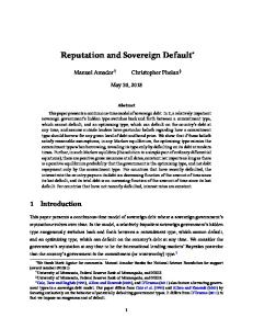
4. Results 4.1 Cycle is not trend Historical decomposition shows that contributions of transitory shock is much larger than that of trend shock (Figure.1). The time series are logged and differenced, as we mentioned section 3.2. Both the cycles of output and external debt are mostly explained by transitory shock (Figure.2). However, debt accumulation when default is mostly explained by trend shock. This indicates that trend shock may be unimportant as cycle, but important as trend supporting continuous accumulation of Argentina’s external debt. Random walk component which is criterion of contributions of trend shock proposed by Aguiar and Gopinath (2007), also implicates the trend shock is much more important than transitory shock (Table.3). The equation of random walk component is given by: 2

2 𝛼𝛼 2 𝜎𝜎𝑔𝑔2 /�1 − 𝜌𝜌𝑔𝑔 � 𝜎𝜎Δ𝜏𝜏 = 2 𝜎𝜎Δ𝑠𝑠𝑠𝑠 [2/(1 + 𝜌𝜌𝑧𝑧 )]𝜎𝜎𝑧𝑧2 + �𝛼𝛼 2 𝜎𝜎𝑔𝑔2 /�1 − 𝜌𝜌𝑔𝑔2 ��

α is labor exponent used in RBC model, but our model and most of structural sovereign default models, do not use

this parameter. We set α = 0.32 or α = 0.68 which are the same values of Aguiar and Gopinath (2007),

Garcia-Cicco, Pancrazi and Uribe (2010) and Chang and Fernández (2013). The result of our estimation is much less than all preceding studies. The model predicts default period completely both 1980s’ and 2000s’. Fluctuations of output and interest rate are well replicated, but more precise replication of external debt fluctuation is left for future research (Figure.2). As a whole, our result implicates that estimation of Garcia-Cicco, Pancrazi and Uribe (2010) and Chang and

Preliminary and incomplete draft Fernández (2013) are correct and robust.

Table.3 Random walk component Our stochastic trend model

Capital income share Random-walk component

α = 0.32 0.005

α = 0.68 0.001

Aguiar and Gopinath

Garcia-Cicco, Pancrazi

Chang and Fernández

(2007)

and Uribe (2010)

(2013)

α = 0.68

0.88 ~ 1.13

Figure.1 Historical decomposition of stochastic trend model

α = 0.32 0.01

α = 0.68 0.18

Preliminary and incomplete draft Figure.2 Fitting of our model

Preliminary and incomplete draft 4.2 The costs of sovereign default of Argentina The estimates of probability of regain an access to international financial market and both asymmetric and proportional domestic costs are much less than conventional calibration of structural sovereign default models. The estimate of discount factor is much less discount factor than DSGE studies on advanced economies, which is consistent with preceding studies of structural sovereign default models. These results are robust since we observe similar output between stochastic trend model and the model with HP-filter trend (Table.4 and Table.5). The reason of our result is that structural estimation captures whole business cycles. Due to the property of the structural sovereign default model, as default costs are smaller, frequency of default increases, which prevents the government to accumulate external debt. The risk neutral lenders know the probability of default is high when the default costs are small, and do not allow the government to borrow huge amount of money. On the other hand, as the probability of reentry is smaller, the government tends to default less frequently since the penalty works long time, which makes external debt stocks relatively large. Less discount factor tends to increase both external debt and default frequency. The government borrows more at good time, and this makes benefit of default larger since default costs are easily compensated by nonfulfillment. As for Argentina economy, external debt stock is large, but default is frequent. Our results, small domestic costs, small probability of reentry and small discount factor accelerate debt accumulation, and decelerate default frequency. Best combination is chosen by simulated tempering SMC-SMC. In terms of log-likelihood value, our result fits actual data better than basic calibrations of Aguiar and Gopinath (2006) and Arellano (2008) (see Table.7). For more equal comparison, we show log-likelihood values calculated under same measurement errors, which are 20% of standard deviation of observables.

Table.4 Posteriors: stochastic trend model β σ r 𝜌𝜌𝑧𝑧 𝜎𝜎𝑧𝑧 θ (1 − 𝜆𝜆𝛼𝛼 ) �1 − 𝜆𝜆𝛽𝛽 �

Discount Factor Risk aversion Risk-free interest rate Persistence of transitory shock SD of transitory shock Probability of reentry Asymmetric Domestic cost Proportional Domestic cost

Distributions

Mean

5%

95%

Uniform Inverse Gamma Inverse Gamma Beta Inverse Gamma Uniform Uniform Uniform

0.830 1.989 0.040 0.868 0.030 0.204 0.0028 0.00065

0.782 1.904 0.038 0.833 0.029 0.196 0.0026 0.00062

0.874 2.087 0.043 0.897 0.031 0.212 0.0029 0.00068

𝜇𝜇𝑔𝑔

Gross mean growth

Uniform

1.0078

1.0002

1.0121

Persistence of trend shock

Uniform

0.249

0.238

0.260

𝜎𝜎𝑔𝑔

SD of trend shock

Uniform

0.0024

0.0023

0.0025

𝜌𝜌𝑔𝑔

Log-likelihood value

-80.18

Preliminary and incomplete draft Table.5 Posteriors: HP-filter detrending β σ r 𝜌𝜌𝑧𝑧 𝜎𝜎𝑧𝑧 θ (1 − 𝜆𝜆𝛼𝛼 ) �1 − 𝜆𝜆𝛽𝛽 �

Discount Factor Risk aversion Risk-free interest rate Persistence of transitory shock SD of transitory shock Probability of reentry Asymmetric Domestic cost Proportional Domestic cost Log-likelihood value

Distributions

Mean

5%

95%

Uniform Inverse Gamma Inverse Gamma Beta Inverse Gamma Uniform Uniform Uniform

0.843 2.01 0.044 0.911 0.033 0.245 0.028 0.0016

0.810 1.91 0.042 0.864 0.032 0.231 0.027 0.0015

0.875 2.103 0.047 0.972 0.035 0.259 0.029 0.0017

-76.25

Table.6 Log-likelihood values under same measurement errors (20% of standard deviation of observables) Our model with HP-filter trend

Aguiar and Gopinath (2006) with HP-filter

Arellano (2008) with HP-filter

-248.77

-534.96

-291.79

5. Conclusions We quantitatively evaluate DSGE model of the emerging economy with microfounded financial imperfection, namely structural sovereign default model. Whether trend is cycle or not, in other words, whether trend shock or transitory shock is important for the business cycles of emerging economies is the lively question since Aguiar and Gopinath (2007).

Estimating RBC using GMM, they insist shock to trend growth rather than transitory

fluctuations around a stable trend are primary source of fluctuations in emerging markets. On the other hand, current studies of estimating RBC with ad-hoc financial imperfection, such as García-Cicco, Pancrazi and Uribe (2010) and Chang and Fernández (2013), emphasize the importance of stationary financial frictions rather than nonstationary trend shock, but they left challenges of microfounded financial imperfection as a further research. Thus, we provide more precise evaluation estimating structural sovereign default model. To obtain more robust and accurate results efficiently, estimation algorithm is simulated tempering SMC-SMC. It explores parameter estimates using whole prior spaces, on the other hand, random walk Metropolis-Hastings algorithm are criticized that parameter draws may have high serial correlation, or may get stuck near local mode. This feature is very important since there is less agreement on some deep parameters such as discount factor, probability of reentry and domestic cost, and more objective estimation is required. Furthermore, we adopt uniform distribution for priors of those important parameters, and secure objective results. As a result, both historical decomposition and random-walk component show that contribution of transitory shock is much larger than that of trend shock. These support the conclusion of García-Cicco, Pancrazi and Uribe (2010) and Chang and Fernández (2013). Furthermore, we show that probability of reentry, both proportional and asymmetric domestic costs are much less than conventional calibration of structural sovereign default studies. Discount factor is approximately 0.8 which is much less than advanced economies. This gives the ground on low discount factor which is usually

Preliminary and incomplete draft justified by circular reasoning within the literatures. We consider that our parameter estimates should be the standard calibration values on Argentina economies. Further research is needed to replicate more external debt accumulation. Estimating Mendoza and Yue (2012), which succeeded to replicate large external debt of Argentina with endogenous domestic cost, is promising. On the other hand, our structural estimation application has large potential to analyze emerging countries further. For example, Uribe and Yue (2006) points out that U.S. monetary policy is the key driver effects on business cycles of emerging economy, but sovereign default models, including this paper, fixed world interest rate. Full-nonlinear multi-country DSGE estimation may enables us to analyze U.S. monetary policy effect more precisely.

Acknowledgements We are thankful for helpful comments from Junko Koeda, Kozo Ueda, Kazufumi Yamaza, Ryo Ishida.

References 1. Aguiar, M., Gopinath, G., 2006. Defaultable debt, interest rates and the current account, Journal of International Economics69, 64-83. 2. Aguiar, M., Chatterjee, S., Cole, H., Stangebye, Z., 2016. Quantitative models of sovereign debt crises, NBER Worlong Paper 22125. 3. Alfaro, L., Kanczuk, F., 2009. Optimal reserve management and sovereign debt. Journal of International Economics 77, 23-36. 4. Amisano, G., Tristani, O., 2010. Euro area inflation persistence in an estimated nonlinear DSGE model. Journal of Economic Dynamics and Control 34, 1837-1858. 5. An, S., Schorfheide, F., 2007. Bayesian Analysis of DSGE Models. Econometric Reviews 26 (2-4), 113-172. 6. Arellano, C., 2008. Default risk and income fluctuations in emerging economies. American Economic Review 98 (3), 690-712. 7. Borensztein, E., Panizza, U., 2011. The Costs of Sovereign Default. IMF Staff Papers 56 (4), 683—741. 8. Boz, E., 2011. Sovereign default, private sector creditors, and IFIs. Journal of International Economics 83, 72-82. 9. Chib, S., Ramamurthy, S., 2010. Tailored randomized block MCMC methods with application to DSGE models. Journal of Econometrics 115, 19-38. 10. Chuan, P., Sturzenegger, F., 2005. Defaults episodes in the 1980s and 1990s: What have we learned?. In Managing Economic Volatility and Crisis, ed. by Aizenman, J., Brian, P. Cambridge-University Press. 11. Cuadra, G., Sanchez, J, M., Sapriza, H., 2010. Fiscal policy and default risk in emerging markets. Review of Economic Dynamics 13, 452-469. 12. Cuadra, G., Sapriza, H., 2008. Sovereign default, interest rates and political uncertainty in emerging markets. Journal of International Economics 76, 78-88. 13. Curdia, V., Reis, R., 2010. Correlated distributions and U.S. business cycles. Working paper.

Preliminary and incomplete draft 14. Durdu, C., B., Nunes, R., Sapriza, H., 2013. News and sovereign default risk in small open economies. Journal of International Economics 91, 1-17. 15. Eaton, J., Gersovitz, M., 1981. Debt with potential repudiation: theoretical and empirical analysis. Review of Economic Studies 48, 289–309. 16. Fernández-Villaverde, J., Rubio-Ramírez, J. F., 2005. Estimating Dynamic Equilibrium Economies: Linear versus Nonlinear Likelihood. Journal of Applied Econometrics 20 (7), 891–910. 17. Fernández-Villaverde, J., Rubio-Ramírez, J. F., 2007. Estimating Macroeconomic Models: A Likelihood Approach. Review of Economic Studies 74 (4), 1059–1087. 18. Flury, T., Shephard, N., 2011. Bayesian inference based only on simulated likelihood: particle filter analysis of dynamic economic models. Econometric Theory 1, 1–24. 19. Gelos, R., G., Sahay, R., Sandleris, G., 2011. Sovereign borrowing by developing countries: What determines market access?. Journal of International Economics 83 (2), 243-254. 20. Flandreau, M., Zumer, F., 2004. The making of global finance 1880-1913. OECD Development Center Research Monograph 21. Gust, C., Lopez-Salido, D., Smith, ME., 2012. The empirical implications of the interest-rate lower bound. Finance and economics discussion series 83, Board of Governors of the Federal Reserve System. 22. Hatchondo, J, C., Martinez, L., 2009. Long-duration bonds and sovereign defaults. Journal of International Economics 79, 117-125. 23. Herbst, E., 2011. Gradient and Hessian-based MCMC for DSGE models. Working paper. 24. Herbst, E., Schorfheide, F., 2014. Sequential Monte Carlo Sampling for DSGE Models. Journal of Applied Econometrics 29, 1073-1098. 25. Hirose, Y., Inoue, A., 2015. The Zero Lower Bound and Parameters Bias in as Estimated DSGE model. Journal of Applied Econometrics 31 (4), 630-651. 26. Kydland and Zarazaga 27. Kohn, R., Giordani, P., Strid, I., 2020. Adaptive hybrid Metropolis-Hastings samples for DSGE models. Scandinavian Working Papers in Economics, No. 724. 28. Martinez, J., V., Sandleris, G., 2011. Is it punishment? Sovereign defaults and the decline in trade. Journal of International Money and Finance 30, 909-930. 29. Malik, S., Pitt, M, K., 2011. Particle filters for continuous likelihood evaluation and maximization. Journal of Econometrics 165, 190-209. 30. Mendoza, E., Yue, V., 2012. A general equilibrium model of sovereign default and business cycles. The Quarterly Journal of Economics, 1-57. 31. Panizza, U., Sturzenegger, F., Zettelmeyer, J., 2009. The Economics and Law of Sovereign Debt and Default. Journal of Economic Literature 47 (3), 651-698. 32. Rose, A., J., 2005. One reason countries pay their debts: renegotiation and international trade. Journal of International Economics 77, 189-206. 33. Schmitt-Grohé, S., Uribe, M., 2004. Solving dynamic general equilibrium models using a second-order approximation to the policy function. Journal of Economic Dynamics and Control 28, 755 – 775.

Preliminary and incomplete draft 34. Schmitt-Grohé, S., Uribe, M., 2012. What’s news in business cycles. Econometrica 80 (6), 2733–2764. 35. Smets, F., Wouters, R., 2003. An Estimated Dynamic Stochastic General Equilibrium Model of the Euro Area. Journal of the European Economic Association 1 (5), 1123-1175. 36. Smets, F., Wouters, R., 2007. Shocks and frictions in US business cycles: a Bayesian DSGE approach. American Economic Review 97 (3), 586-606. 37. Uribe, M., Yue, V., Z., 2004. Country spreads and emerging countries: Who drives whom?. Journal of International Economics 69, 6–36.

Preliminary and incomplete draft

Appendix: Algorithms in detail Algorithm 0: Policy Function Iteration 1. 2. 3. 4.

Guess a value function 𝑉𝑉 𝑜𝑜 (B𝑡𝑡 , y𝑡𝑡 ) and bond price 𝑞𝑞(B𝑡𝑡+1 , 𝑦𝑦𝑡𝑡 ) At each (B𝑡𝑡+1 , 𝑦𝑦𝑡𝑡 ), update 𝑣𝑣 𝑑𝑑 (𝑦𝑦𝑡𝑡 ) and 𝑣𝑣 𝑐𝑐 (B𝑡𝑡 , y𝑡𝑡 )

Update 𝑉𝑉 𝑜𝑜 (B𝑡𝑡 , y𝑡𝑡 ), the default rule, the implied ex ante default probability, and the bond price function

Iterate step 2 and step3 until convergence

Algorithm 1: Simulated tempering SMC 1. Initialization Draw 𝜃𝜃1𝑖𝑖 , ⋯ 𝜃𝜃1𝑁𝑁 from the prior π(𝜃𝜃1 ) and set 𝑤𝑤1𝑖𝑖 = 𝑁𝑁 −1, i = 1, ⋯ N.

2. Recursion For n = 2, ⋯ , 𝑁𝑁𝜙𝜙 (a) Correction

Reweight the particles from stage n − 1 by defining the incremental and normalized weights by 𝜙𝜙𝑛𝑛 −𝜙𝜙𝑛𝑛−1

𝑖𝑖 calculating incremental and normalized weights 𝑤𝑤 �𝑛𝑛𝑖𝑖 = �𝑝𝑝�𝑌𝑌|𝜃𝜃𝑛𝑛−1 �� 1 𝑖𝑖 𝑖𝑖 𝐸𝐸𝜋𝜋𝑛𝑛 [ℎ(𝜃𝜃)] is approximated to ℎ�𝑛𝑛,𝑁𝑁 = 𝑁𝑁 ∑𝑁𝑁 𝑖𝑖=1 ℎ�𝜃𝜃𝑛𝑛−1 � 𝑊𝑊𝑛𝑛

�𝑛𝑛𝑖𝑖 = and 𝑊𝑊

𝑖𝑖 � 𝑛𝑛𝑖𝑖 𝑊𝑊𝑛𝑛−1 𝑤𝑤 1 𝑁𝑁 𝑖𝑖 𝑖𝑖 ∑𝑖𝑖=1 𝑤𝑤 � 𝑛𝑛 𝑊𝑊𝑛𝑛−1 𝑁𝑁

.

(b) Selection Compute the effective sample size 𝐸𝐸𝐸𝐸𝐸𝐸𝑛𝑛 = If 𝜌𝜌�𝑛𝑛 = 1, where 𝜌𝜌�𝑛𝑛 = ℒ{𝐸𝐸𝐸𝐸𝐸𝐸𝑛𝑛 < 0.5𝑁𝑁}

𝑁𝑁

.

2 1 �𝑖𝑖𝑛𝑛 � � � ∑𝑁𝑁 �𝑊𝑊 𝑁𝑁 𝑖𝑖=1

𝑁𝑁 𝑖𝑖 �𝑛𝑛𝑖𝑖 �𝑁𝑁 . Let 𝑊𝑊𝑛𝑛𝑖𝑖 = 1. Resample the particles by multinomial resampling, � 𝜃𝜃� �𝑖𝑖=1 = �𝜃𝜃𝑛𝑛−1 , 𝑊𝑊 𝑖𝑖=1

If 𝜌𝜌�𝑛𝑛 = 0

𝑖𝑖 �𝑛𝑛𝑖𝑖 . 𝐸𝐸𝜋𝜋 [ℎ(𝜃𝜃)] is approximated to ℎ�𝑛𝑛,𝑁𝑁 = Let 𝜃𝜃�𝑛𝑛𝑖𝑖 = 𝜃𝜃𝑛𝑛−1 and 𝑊𝑊𝑛𝑛𝑖𝑖 = 𝑊𝑊 𝑛𝑛

1

𝑁𝑁

𝑖𝑖 � 𝑖𝑖 ∑𝑁𝑁 𝑖𝑖=1 ℎ�𝜃𝜃𝑛𝑛 � 𝑊𝑊𝑛𝑛 .

(c) Mutation Propagate the particles �𝜃𝜃�i , 𝑊𝑊𝑛𝑛𝑖𝑖 � by Metropolis-Hastings algorithm with transition density 𝜃𝜃𝑛𝑛𝑖𝑖 ~𝐾𝐾𝑛𝑛 �𝜃𝜃𝑛𝑛 |𝜃𝜃�𝑛𝑛𝑖𝑖 ; 𝜉𝜉𝑛𝑛 � and stationary 𝜋𝜋𝑛𝑛 (𝜃𝜃) (See Algorithm 2). 𝐸𝐸𝜋𝜋𝑛𝑛 [ℎ(𝜃𝜃)] is approximated to ℎ�𝑛𝑛,𝑁𝑁 =

3. Final importance sampling approximation of 𝐸𝐸𝜋𝜋 [ℎ(𝜃𝜃)] 𝑖𝑖 𝑖𝑖 When n = 𝑁𝑁𝜙𝜙 , ℎ�𝑁𝑁𝜙𝜙 ,𝑁𝑁 = ∑𝑁𝑁 𝑖𝑖=1 ℎ �𝜃𝜃𝑁𝑁𝜙𝜙 � 𝑊𝑊𝑁𝑁𝜙𝜙

1

𝑁𝑁

𝑖𝑖 𝑖𝑖 ∑𝑁𝑁 𝑖𝑖=1 ℎ�𝜃𝜃𝑛𝑛 � 𝑊𝑊𝑛𝑛 .

Preliminary and incomplete draft Algorithm 2: Particle mutation; Prior to executing Algorithm 1 1. Generate Blocks Randomly 𝑁𝑁

𝜙𝜙 Generate a sequence of random partitions {𝐵𝐵𝑛𝑛 }𝑛𝑛=2 of 𝜃𝜃𝑛𝑛 into 𝑁𝑁𝑏𝑏𝑏𝑏𝑏𝑏𝑏𝑏𝑏𝑏𝑏𝑏 equally sized blocks, denoted by

∗ ∗ ∗ 𝜃𝜃𝑛𝑛,𝑏𝑏 . Let 𝜃𝜃𝑛𝑛,𝑏𝑏 and Σ𝑛𝑛,𝑏𝑏 be the partitions of 𝜃𝜃𝑛𝑛∗ and Σ𝑛𝑛∗ that correspond to the subvector 𝜃𝜃𝑛𝑛,𝑏𝑏 .

2. MH-steps: For i = 1 to M:

For b = 1 to 𝑁𝑁𝑏𝑏𝑏𝑏𝑏𝑏𝑏𝑏𝑏𝑏𝑏𝑏 :

(a) Proposal Draw

Draw proposal ϑ𝑏𝑏 from the mixture distribution

𝑖𝑖 𝑖𝑖 𝑖𝑖 ∗ ∗ ∗ ϑ𝑏𝑏 |�𝜃𝜃𝑛𝑛,𝑏𝑏,𝑚𝑚−1 , 𝜃𝜃𝑛𝑛,−𝑏𝑏,𝑚𝑚 , 𝜃𝜃𝑛𝑛,𝑏𝑏 , Σ𝑛𝑛,𝑏𝑏 �~𝛼𝛼𝛼𝛼�𝜃𝜃𝑛𝑛,𝑏𝑏,𝑚𝑚−1 , 𝑐𝑐𝑛𝑛2 Σ𝑛𝑛,𝑏𝑏 �+ 1−𝛼𝛼 2

∗ ∗ 𝑁𝑁�𝜃𝜃𝑛𝑛,𝑏𝑏 , 𝑐𝑐𝑛𝑛2 Σ𝑛𝑛,𝑏𝑏 �

1−𝛼𝛼 2

𝑖𝑖 ∗ 𝑁𝑁 �𝜃𝜃𝑛𝑛,𝑏𝑏,𝑚𝑚−1 , 𝑐𝑐𝑛𝑛2 𝑑𝑑𝑑𝑑𝑑𝑑𝑑𝑑�Σ𝑛𝑛,𝑏𝑏 �� +

(b) Solve the model and evaluate the proposal Solve the model (See Section.) Evaluate the likelihood (c) Accept or Reject Calculate α�ϑ𝑏𝑏 |𝜃𝜃𝑖𝑖𝑛𝑛,𝑏𝑏,𝑚𝑚−1 , 𝜃𝜃𝑖𝑖𝑛𝑛,−𝑏𝑏,𝑚𝑚, 𝜃𝜃∗𝑛𝑛,𝑏𝑏, Σ∗𝑛𝑛,𝑏𝑏 � and let

= 𝑚𝑚𝑚𝑚𝑚𝑚 �1,

𝑝𝑝𝜙𝜙𝑛𝑛 �𝑌𝑌|ϑ𝑏𝑏 , 𝜃𝜃𝑖𝑖𝑛𝑛,−𝑏𝑏,𝑚𝑚�𝑝𝑝�ϑ𝑏𝑏 , 𝜃𝜃𝑖𝑖𝑛𝑛,−𝑏𝑏,𝑚𝑚�/𝑞𝑞�ϑ𝑏𝑏 |𝜃𝜃𝑖𝑖𝑛𝑛,𝑏𝑏,𝑚𝑚−1 , 𝜃𝜃𝑖𝑖𝑛𝑛,−𝑏𝑏,𝑚𝑚, 𝜃𝜃∗𝑛𝑛,𝑏𝑏, Σ∗𝑛𝑛,𝑏𝑏 �

� 𝑝𝑝𝜙𝜙𝑛𝑛 �𝑌𝑌|𝜃𝜃𝑖𝑖𝑛𝑛,𝑏𝑏,𝑚𝑚−1, 𝜃𝜃𝑖𝑖𝑛𝑛,−𝑏𝑏,𝑚𝑚�𝑝𝑝�𝜃𝜃𝑖𝑖𝑛𝑛,𝑏𝑏,𝑚𝑚−1 , 𝜃𝜃𝑖𝑖𝑛𝑛,−𝑏𝑏,𝑚𝑚 �/𝑞𝑞�𝜃𝜃𝑖𝑖𝑛𝑛,𝑏𝑏,𝑚𝑚−1|ϑ𝑏𝑏 , 𝜃𝜃𝑖𝑖𝑛𝑛,−𝑏𝑏,𝑚𝑚, 𝜃𝜃∗𝑛𝑛,𝑏𝑏 , Σ∗𝑛𝑛,𝑏𝑏 �

𝑖𝑖 𝑖𝑖 ∗ ∗ ϑ𝑏𝑏 𝑤𝑤𝑤𝑤𝑤𝑤ℎ 𝑝𝑝𝑝𝑝𝑝𝑝𝑝𝑝𝑝𝑝𝑝𝑝𝑝𝑝𝑝𝑝𝑝𝑝𝑝𝑝𝑝𝑝 α�ϑ𝑏𝑏 |𝜃𝜃𝑛𝑛,𝑏𝑏,𝑚𝑚−1 , 𝜃𝜃𝑛𝑛,−𝑏𝑏,𝑚𝑚 , 𝜃𝜃𝑛𝑛,𝑏𝑏 , Σ𝑛𝑛,𝑏𝑏 � 𝑖𝑖 𝜃𝜃𝑛𝑛,𝑏𝑏,𝑚𝑚 =� 𝑖𝑖 𝜃𝜃𝑛𝑛,𝑏𝑏,𝑚𝑚−1 𝑜𝑜𝑜𝑜ℎ𝑒𝑒𝑒𝑒𝑒𝑒𝑒𝑒𝑒𝑒𝑒𝑒𝑒𝑒

3. Final step

𝑖𝑖 𝑖𝑖 Let 𝜃𝜃𝑛𝑛,𝑏𝑏= 𝜃𝜃𝑛𝑛,𝑏𝑏,𝑀𝑀

Algorithm 3: Adaptive particle mutation; Prior to Step 1 of Algorithm 2 1. Importance sampling approximation Calculate importance sampling approximations 𝜃𝜃�𝑛𝑛 and Σ�𝑛𝑛 of 𝐸𝐸𝜋𝜋𝑛𝑛 [𝜃𝜃] and 𝑉𝑉𝜋𝜋𝑛𝑛 [𝜃𝜃] according to particles 𝑖𝑖 �𝑛𝑛𝑖𝑖 �𝑁𝑁 . �𝜃𝜃𝑛𝑛−1 , 𝑊𝑊 𝑖𝑖=1

2. Adjusting scaling factor Calculate the average rejection rate 𝑅𝑅�𝑛𝑛−1 �𝜉𝜉̂𝑛𝑛−1 �, based on the Mutation step in iteration n − 1, across 𝑁𝑁𝑏𝑏𝑏𝑏𝑏𝑏𝑏𝑏𝑏𝑏𝑏𝑏 .

Adjusting scaling factor following 𝑐𝑐̂2 = 𝑐𝑐 ∗ and 𝑐𝑐̂𝑛𝑛 = 𝑐𝑐̂𝑛𝑛−1 𝑓𝑓 �1 − 𝑅𝑅�𝑛𝑛−1 �𝜉𝜉̂𝑛𝑛−1 ��, 𝑒𝑒 16(𝑥𝑥−0.25)

where 𝑓𝑓(𝑥𝑥) = 0.95 + 0.10 1+𝑒𝑒 16(𝑥𝑥−0.25)

Preliminary and incomplete draft 3. Replacing ′

′ Replace 𝜉𝜉𝑛𝑛 with 𝜉𝜉̂𝑛𝑛 = �𝑐𝑐̂𝑛𝑛 , 𝜃𝜃�𝑛𝑛 , 𝑣𝑣𝑣𝑣𝑣𝑣ℎ�Σ�𝑛𝑛 � � .

Algorithm 4: Particle filter 1. Initialization 𝑗𝑗

𝑗𝑗

Draw the initial particles from 𝑠𝑠0 ~𝑝𝑝(𝑠𝑠0|𝜃𝜃) and set 𝑊𝑊0 = 1.

2. Recursion For t = 1, ⋯ , T (a) Forecasting 𝑠𝑠𝑡𝑡

𝑗𝑗

𝑗𝑗

Propagate the particles �𝑠𝑠𝑡𝑡−1 , 𝑊𝑊𝑡𝑡−1 � by simulating state-transition equation:

(b) Forecasting

𝑦𝑦𝑡𝑡

𝑗𝑗

𝑗𝑗

𝑗𝑗

𝑗𝑗

𝜖𝜖𝑡𝑡 ~𝐹𝐹𝜖𝜖 (∙; 𝜃𝜃)

𝑠𝑠̃𝑡𝑡 = Φ�𝑠𝑠𝑡𝑡−1 , 𝜖𝜖𝑡𝑡 ; 𝜃𝜃�,

Calculate the incremental weights: 𝑗𝑗

𝑗𝑗

𝑤𝑤 �𝑡𝑡 = 𝑝𝑝�𝑦𝑦𝑡𝑡 |𝑠𝑠̃𝑡𝑡 , 𝜃𝜃�

Approximate predictive density 𝑝𝑝(𝑦𝑦𝑡𝑡 |𝑌𝑌1:𝑡𝑡−1 , 𝜃𝜃) as follows: 𝑝𝑝(𝑦𝑦𝑡𝑡 |𝑌𝑌1:𝑡𝑡−1 , 𝜃𝜃) = (c) Updating

1

𝑁𝑁𝑓𝑓𝑓𝑓𝑓𝑓𝑓𝑓𝑓𝑓𝑓𝑓

𝑁𝑁𝑓𝑓𝑓𝑓𝑓𝑓𝑓𝑓𝑓𝑓𝑓𝑓

𝑗𝑗

𝑗𝑗

� 𝑤𝑤 �𝑡𝑡 𝑊𝑊𝑡𝑡−1 𝑗𝑗=1

Calculate the normalized weights �𝑡𝑡𝑗𝑗 = 𝑊𝑊

(d) Selection

𝑗𝑗

𝑗𝑗

� 𝑡𝑡 𝑊𝑊𝑡𝑡−1 𝑤𝑤

𝑁𝑁 1 𝑗𝑗 𝑗𝑗 ∑ 𝑓𝑓𝑓𝑓𝑓𝑓𝑓𝑓𝑓𝑓𝑓𝑓 � 𝑡𝑡 𝑊𝑊𝑡𝑡−1 𝑁𝑁𝑓𝑓𝑓𝑓𝑓𝑓𝑓𝑓𝑓𝑓𝑓𝑓 𝑗𝑗=1 𝑤𝑤

If 𝜌𝜌�𝑡𝑡 = 1, where 𝜌𝜌�𝑡𝑡 = ℒ{𝐸𝐸𝐸𝐸𝐸𝐸𝑡𝑡 < 0.5𝑁𝑁}, where 𝐸𝐸𝐸𝐸𝐸𝐸𝑡𝑡 = 𝑀𝑀/ �𝑁𝑁

1

𝑓𝑓𝑓𝑓𝑓𝑓𝑓𝑓𝑓𝑓𝑓𝑓

𝑗𝑗 𝑁𝑁𝑓𝑓𝑓𝑓𝑓𝑓𝑓𝑓𝑓𝑓𝑓𝑓

Resample the particles by multinomial resampling, �𝑠𝑠𝑡𝑡 �𝑗𝑗=1

If 𝜌𝜌�𝑡𝑡 = 0

𝑗𝑗

𝑗𝑗

𝑗𝑗

𝑗𝑗

The approximation of the likelihood function is given by: 𝑇𝑇

1

𝑁𝑁𝑓𝑓𝑓𝑓𝑓𝑓𝑓𝑓𝑓𝑓𝑓𝑓

𝑗𝑗

𝑗𝑗

𝑝𝑝̂ (𝑌𝑌1:𝑇𝑇 |𝜃𝜃) = � � � 𝑤𝑤 �𝑡𝑡 𝑊𝑊𝑡𝑡−1 � 𝑁𝑁𝑓𝑓𝑓𝑓𝑓𝑓𝑓𝑓𝑓𝑓𝑓𝑓 𝑡𝑡=1

𝑗𝑗=1

𝑁𝑁

𝑗𝑗 � 𝑗𝑗 𝑓𝑓𝑓𝑓𝑓𝑓𝑓𝑓𝑓𝑓𝑓𝑓 𝑗𝑗 = �𝑠𝑠̃𝑡𝑡 , 𝑊𝑊 . Let 𝑊𝑊𝑡𝑡 = 1. 𝑡𝑡 �𝑗𝑗=1

�𝑡𝑡 . Let 𝑠𝑠𝑡𝑡 = 𝑠𝑠̃𝑡𝑡 and 𝑊𝑊𝑡𝑡 = 𝑊𝑊

3. Likelihood approximation

2

𝑁𝑁

𝑗𝑗 𝑓𝑓𝑓𝑓𝑓𝑓𝑓𝑓𝑓𝑓𝑓𝑓 ∑𝑗𝑗=1 �𝑊𝑊𝑡𝑡 � �