Speaker Adaptation with an Exponential Transform Daniel Povey, Geoffrey Zweig, Alex Acero Microsoft Research, Microsoft, One Microsoft Way, Redmond, WA 98052, USA
[email protected],
[email protected],
[email protected]
Abstract—In this paper we describe a linear transform that we call an Exponential Transform (ET), which integrates aspects of CMLLR, VTLN and STC/MLLT into a single transform with jointly trained components. Its main advantage is that a very small number of speakerspecific parameters is required, thus enabling effective adaptation with small amounts of speaker specific data. Our formulation shares some characteristics of Vocal Tract Length Normalization (VTLN), and is intended as a substitute for VTLN. The key part of the transform is controlled by a single speaker-specific parameter that is analogous to a VTLN warp factor. The transform has non-speaker-specific parameters that are learned from data, and we find that the axis along which male and female speakers differ is automatically learned. The exponential transform has no explicit notion of frequency warping, which makes it applicable in principle to non-standard features such as those derived from neural nets, or when the key axes may not be male-female. Based on our experiments with standard MFCC features, it appears to perform better than conventional VTLN.
I. I NTRODUCTION Vocal Tract Length Normalization (VTLN) [1], [2], [3], [4] is a standard feature of modern speech recognition systems. The basic idea is to scale the frequency axis on a per-speaker basis so as to normalize the formant positions. These can vary by about 20% between speakers [5] because gender and other factors affect the length of the vocal tract. Currently, the most commonly used approach to VTLN operates by repeating feature extraction multiple times (e.g. 20 times), for a discrete set of warping factors, and selecting the warp that provides the highest likelihood features with respect to a simple model. Linear-transform based implementations of VTLN have been investigated by various authors [1], [6], [7], [8], [9], [10]. The basic idea is to approximate the VTLN frequency warping by a linear transformation of the MFCC or PLP features. In some cases [1], [6], [8] this is based on an analysis that leads to a formula; in other cases [7], [9] it is based on linear transforms which are trained to approximate the conventional feature-level VTLN warping. At test time these techniques are equivalent to Constrained MLLR (CMLLR) [11] but choosing from a fixed set of transforms. Note that when applying a linear transform x → Ax+b, one should add log | det A| to the log-likelihoods, as dictated by the identity N (Ax + b; µ, Σ)| det A| = N (x; A−1 µ − A−1 b, A−1 ΣA−T ), (1) where the right hand side represents the “model-space” interpretation of the transformation. This is referred to as Jacobian compensation, since A is the Jacobian of the transformation. In practice not all authors include the Jacobian term; see [10] for an investigation of the effect of this. In conventional (feature-level) VTLN, cepstral variance normalization generally has to be applied because there is no natural way to do Jacobian compensation [9]. Linear-transform based approaches to VTLN have generally been found to be about as effective as standard VTLN, while being more efficient to implement. Typically about 20 transforms would be estimated at training time, and at test time one would select the best one of these based on the likelihood assigned by the model to the transformed data.
A natural question to ask is: once we are working in a linear transform based framework, why not estimate the (say) 20 transforms in a purely data-driven way, without reference to the original VTLN? For large training datasets, the number of parameters to estimate is relatively quite modest so such an approach may be feasible. One way to do this would be in a K-means framework, iteratively estimating transforms and reassigning speakers to transforms. One might even envision initializing these clusters from the VTLN warp factors, thereby nudging the system towards normal VTLN. However, our experiments along these lines (not described further) were not successful, motivating a more powerful approach. II. T HE E XPONENTIAL T RANSFORM A. Basic Idea We now turn to a form of transform which will give us a continuously varying set of transforms controlled by a single parameter. We first consider a pure linear transform; later an offset term will be introduced. The most basic form of the idea is to use a transform of the form A(s) = exp(t(s) A), (2) where t(s) is a speaker-specific scalar that may be positive or negative and that is analogous to the log of a VTLN warp factor, A is a global parameter matrix that is learned from data, and A(s) is the speaker specific “exponential transform”. Here, exp is the matrix exponential function, which is defined (for square matrices only) by the Taylor series expansion: ∞ X 1 n exp(M) ≡ M , (3) n! n=0
with Mn defined in the obvious way as a product of M with itself n times and M0 being the identity matrix I. Thus, if the entries in M are small, we obtain a transform which is a small delta on the identity matrix. The attraction of this functional form is that the family of functions is closed under matrix multiplication, i.e. the product of two warping matrices is still a warping matrix. B. Full Version We turn now to an extension of the basic transform which addresses the further normalization issues of mean normalization and feature rotation. We augment the d dimensional input vector x with a one to form a vector x+ , and denote the speaker-specific transform with W(s) . The “complete” exponential transform (ET) is: W(s) = D(s) exp(t(s) A)B,
(4)
where D(s) handles mean offsets (and, at test time, diagonal scaling), the middle factor with the exp is the core “exponential transform” part, and B corresponds to MLLT/STC [12], [13]. Any quantities without the superscript s are globally shared. The dimensions are D(s) ∈ Rd×(d+1) , A ∈ R(d+1)×(d+1) , and B ∈ R(d+1)×(d+1) . Reflecting its mean-offset function, D(s) is a matrix with ones along a d × d diagonal, unconstrained entries in the last column, and zeros elsewhere. At test time, we optionally allow unconstrained
entries on the diagonals, but not at training time as this significantly complicates the reestimation formulae. The intuition behind adding the D(s) and B components is that if we want the factor exp(t(s) A) to model a VTLN-like transform, which might correspond to a relatively subtle difference in the features, we need to normalize for gross effects such as speakerdependent offsets and global correlations between parameters. Otherwise it is more likely that the central factor exp(t(s) A) would learn instead to model these types of effects; by modeling such effects explicitly, we free the exponential term to model the effects that cannot modeled by B and D(s) . We emphasize that, like linear VTLN, ET is a specially constrained form of CMLLR. III. M ODEL E STIMATION A. Overview
•
Initialize the global parameters A and B For a number of training iterations: – Compute t(s) and D(s) for the training speakers – Update the model (means, variances, etc.) – On early iterations (e.g. the first 15 iterations), alternately: ∗ Update the matrix A, or: ∗ Update the matrix B.
•
Compute a speaker independent model using just (the first d rows of) B as the feature-space transform.
The speaker independent model has the same mixture-of-Gaussians structure as the final speaker-adapted model, and is computed in one pass using Gaussian-level alignments from the speaker-adapted model. It is used at test time for the first-pass decoding and to obtain Gaussian-level alignments for estimating the transform. B. Summary of notation • • •
• • • • •
•
• •
X
=
The feature dimension is d. We assume zero-based indexing of vectors and matrices. We use xt for the unadapted features on time t. We don’t have an index for the utterance (we just assume distinct utterances have differently numbered time indices). x+ means the vector x with a 1 appended to it. A− , where A is a matrix, means A with its last row removed. A+ , means A with a row with value 0 0 . . . 1 appended. A(+0) , means A with a zero-valued row appended. Gaussian mixture components in a HMM-GMM system are indexed j, m where j is the state and m is the mixture component. The means and (diagonal) variances are µjm and Σjm , with 2 σjmi as the i’th variance component. The Gaussian-level posteriors on time t are γjm (t). Unless otherwise defined, mi is the i’th row of M (viewed as a column vector), and mi,j is its i, j’th element.
C. Definition of CMLLR statistics The sufficient statistics for CMLLR (for a particular speaker) are: X γjm (t) (5) β= t,j,m
+ γjm (t)Σ−1 jm µjm xt
T
(6)
t,j,m
Gi
X
=
γjm (t)
t,j,m
1 +T x+ t xt 2 σjmi
(7)
for 0 ≤ i < d, and the auxiliary function is: −
Q(W) = tr(KT W) + log | det( WT )| −
1 2
D. Manipulations of CMLLR statistics
PD
i=1
wiT Gi wi (8)
It will be necessary in our estimation algorithms to apply a transform in the feature space to CMLLR statistics; this is done as follows. Let M ∈ R(d+1)×(d+1) be a matrix with last row 0 0 . . . 1 that represents an affine transform. We do as follows, which is equivalent to having pre-multiplied x+ by M while collecting the statistics: K
At training time we need to compute the global parameters A and B, and also train a model on suitably adapted features. The objective function we optimize is the data likelihood; the procedure is based on Expectation-Maximization (E-M). An overview of the training procedure is: •
K
Gi
← ←
KMT
(9) T
MGi M .
(10)
Applying a transform in the model space to some statistics is done as follows. Let W ∈ Rd×(d+1) be the affine transform. The modelspace transformation can only be done if W is a diagonal transform, i.e. W = [M b] with M diagonal. We’ll write the (i, i)’th element of M as mi . The transform corresponds to setting xi ← mi xi + bi . After working out how to equivalently apply this transform to the means and variances and obtaining the corresponding transforms on K and Gi , we get as follows. The elements of K change with: ki,j ← mi ki,j − mi bi gi,d,j ,
(11)
where the index d is the feature dimension, and then the matrices Gi are scaled with: Gi ← m2i Gi . (12) E. Computing the matrix exponential function For a review of ways to compute the matrix exponential function, see [14]. The method we used is one of the simpler methods discussed there. Suppose we are computing exp(M). Define P = 2−N M. We choose the smallest integer N ≥ 0 such that ||P|| < 0.1 (using the Frobenius norm). The method is a slight twist on the identity N exp(P)2 = exp(M), using successive squaring to compute the power. Define B0 = exp(P) − I, computed with: B0 =
K X 1 n P , n! n=1
(13)
the series is truncated when we detect that adding the latest term has not caused any change in B0 (we remember the number of terms as K). Then we use the recursion, for 1 ≤ n ≤ N , Bn = Bn−1 Bn−1 + 2Bn−1 ,
(14)
and the answer is given by exp(M) = BN + I. F. Reverse differentiating through the matrix exponential function In this section we define for later use a function exp-backprop, of the form ˆ = M, ˆ exp-backprop(M, X) (15) ˆ are the derivatives of scalar f = where the elements of M T ˆ tr(X exp(M)) w.r.t. the corresponding elements of M. We assume that the intermediate quantities used while computing the matrix exponential function exp(M) (as described in the previous section) are available. We are going backwards through that computation
ˆ N = X. ˆ Then for n = computing derivatives. We first set B N −1, N −2, . . . , 0 we do: ˆn = B ˆ n+1 BTn + BTn B ˆ n+1 + 2B ˆ n+1 . B
(16)
ˆ and we will do so with Next we want to compute P, ˆ = P
K X
ˆ n, P
(17)
n=1
ˆ n is the part of the derivative arising from the n’th term of where P ˆ1 = B ˆ 0 , and for 2 ≤ n ≤ K, the truncated Taylor series 13. We set P let ˆn = 1 P ˆ n−1 AT + 1 An−1 T B ˆ 0, P (18) n n! where it is convenient to cache the powers of A from the forward ˆ ˆ = 1N P. computation. The final answer is given by M 2
G. Computing the speaker-specific transforms In this section we describe how to compute the speaker-specific parameters t(s) and D(s) , given the sufficient statistics K, Gi and β. At training time these statistics are computed with Gaussianlevel alignments given by the previous iteration’s speaker-specific transforms W(s) . At test time the Gausian-level alignments are computed using features transformed only with B, and the speakerindependent model trained using single-pass retraining with features transformed only with B. We will omit the speaker superscript s. We first initialize t ← 0 and D ← [I 0]. Then we apply B as a feature-space transform to the statistics as described in Section III-D. We next do several iterations of update (we used three iterations). On each iteration we first reestimate D and then re-estimate t. 1) Updating D: In the update of D, we first estimate a transform D′ that will go to the right of any existing transform D, and then modify D to take into account the new transform D′ . We estimate D′ via Maximum Likelihood from K, Gi and β as either an offsetonly CMLLR transform (at training time) or a diagonal CMLLR + transform (at test time). We then set D ← DD′ (the meaning of + was explained in Section III-B), and then apply D′ as a modelspace transformation to the statistics K and Gi as described in Section III-D. 2) Updating t: The update for t is similar to the update for D in that we always estimate an “incremental part” t′ and add this to t. To compute t′ we do a single iteration of Newton’s method , starting from t′ = 0. The update formulas are as follows. First define J ∈ Rd×(d+1) by: J = K − S, (19) where the i’th row si of S is the same as the i’th row gii of Gi . This equals the auxiliary function derivative w.r.t exp(t′ A)− , ignoring the log determinant. We will be maximizing the quadratic function 2 f (t′ ) = at′ − 12 bt′ , with a
=
tr(JT A− ) + β tr(A)
(20)
b
=
(21)
b1
=
b1 − b2 ! d−1 X T ai Gi ai
b2
=
i=0 T
tr(J (AA)− )
matrix exp(t′ A) as a feature-space transformation to the statistics as decribed in Section III-D. H. Updating B The accumulation and update formulas for B are based on those for MLLT (equivalently, global STC). Defining x′ as W(s) x+ , i.e. the current transformed features, we accumulate the sufficient statistics (for 0 ≤ i < d), Gi =
X γjm (t) ` ´` ´T µjm − x′ µjm − x′ , 2 σ jmi t
(24)
P and β = t γjm (t). Let the result of the MLLT/STC update be the feature transformation matrix C ∈ Rd×d , which we optimize starting from C = I using the formulas from [15, Appendix A]. For convenience, we them here. The auxiliary function is P repeat T β log | det C| − 21 d−1 i=0 ci Gi ci . To maximize it, for a number of iterations (e.g. 10), we do as follows: for 0 ≤ i < d, F
←
ci
←
C−T s
β G−1 i fi . fiT G−1 i fi
(25) (26)
Let Cf be C extended with an extra row and column, with zeros except for a 1 in position (d, d). After estimating C we do as follows: • •
•
Transform the model by setting µjm ← Cµjm Transform all the current speaker transforms by setting W(s) ← CW(s) Set A ← Cf AC−1 f , and B ← Cf B.
I. Updating A The statistics for updating the matrix A are functions of the standard CMLLR statistics for the training speakers. These CMLLR statistics are computed with Gaussian alignments obtained with features transformed with W(s) , but the statistics themselves contain the original features x, not the transformed features. For each training speaker s, let the CMLLR statistics accumulated as in Section III-C be K(s) , G(s) and β. Using the current values of D(s) and B, apply B as a feature transform to the statistics and apply D(s) as a model-space transform to the statistics, as described ˜ (s) and in Section III-D. Let us write the transformed statistics as K (s) ˜ . Define G i X(s) = exp(t(s) A).
(27)
ˆ (s) , using notation We will write the derivative of Q w.r.t. X(s) as X (s) where x ˆi,j = ∂Q . We have (s) ∂xij
“ ”(+0) ˆ (s) = K ˜ (s) − S(s) X i
(28)
(22)
where (+0) means appending a zero row, and the i’th row of S(s) is given by: (s) ˜ (s) c(s) . si = G (29) i i
(23)
The derivative of Q(s) w.r.t A is given by:
where ai is the i’th row of A. To ensure the correct sign of update even in pathological cases far from convergence, we replace b1 − b2 with b1 −min(0.8b1 , b2 ). We have never seen this flooring take place in practice. We set t′ = a/b. We then set t ← t + t′ , and apply the
ˆ (s) = t(s) exp-backprop(t(s) A, X ˆ (s) ). A
(30)
The statistics for updating A are written as follows, where summations over s are over all training speakers. The index i takes values
0 ≤ i < d. X
β (s)
(31)
t(s) β (s)
(32)
s
βt =
X s
ˆ = A
X
ˆ (s) A
(33)
s
Gi =
X s
t(s)
“ 2
”
˜ (s) + max(g (s) − k(s) , 0)ei eTi , (34) G i i,i,i i,i
where ei is the unit vector in the i’th dimension. Note that Gi is not the same as the Gi quantities for the B update or the speaker(s) dependent Gi quantities in the CMLLR statistics. The (weak-sense) auxiliary function we at test time is a quadratic function with Poptimize T a G quadratic part − 12 d−1 i ai , and a derivative (at the current i i=0 ˆ T + βt I; the βt I comes from the log value of A) given by H = A determinant. The update equation is, for 0 ≤ i < d, ai ← ai + G−1 i hi
We then normalize A to have unit Frobenius norm; this keeps the t(s) values in a more consistent range from run to run (it doesn’t affect the actual transforms produced by the method). IV. BASELINE VTLN IMPLEMENTATION As the first element of our baseline VTLN implementation we implemented the standard, feature-level form of VTLN. This operates by shifting the locations of the center frequencies of the triangular mel bins during the MFCC computation. The warping function is as diagrammed in Figure 1. The two solid lines are examples of warping functions for warping factors greater than, and less than, one. The longest, central line segment always “points” at the origin. Ours is similar to the approach used in the Attila speech recognition toolkit [16], which uses a bilinear function with the property that the inverse of each function is also in the functional family1 ; it handles the upper frequency cutoff differently from HTK [17], in which the knee is always at the same point on the x-axis. Our function is similar to HTK in that it also supports a lower cutoff (this would normally be zero if the lower frequency cutoff for the mel-bin computation was zero). In our experiments, the lower cutoff was 100 and the upper cutoff was always 600 Hz lower than the Nyquist frequency. We implemented linear VTLN (LVTLN) in a way quite similar to [9], except that the linear functions are implemented as follows. On a small subset of data (the same for all warp factors), we compute the original features xt and the warped features ytα , warped with warping factor α as described in the previous paragraph. We used 31 separate warping factors: 0.85, 0.86, . . . 1.15. For each warping Kingsbury, personal communication
Upper cutoff
Lower cutoff Mel bin cutoff
un-warped frequency Fig. 1.
VTLN warping function
(35)
where ai and hi are the i’th rows of A and H, viewed as column vectors; the last row of A is not updated (it is always zero). The P −1 T auxiliary function improvement is 12 d−1 i=0 hi Gi hi . This should generally decrease as training progresses. We want to keep the warp factors t(s) “centered” at training time so that they average to zero; this makes them more consistent between training runs, and makes the approximations we used in deriving the estimation formulas for A more valid (since we ensure smaller values of t(s) ). To do this, after updating A we take the “average part” of exp(t(s) A), and put it into B. The update equation is: „ « βt B ← exp A B. (36) β
1 Brian
Nyquist
warped frequency
β =
factor, we estimate a CMLLR matrix Wα to minimize the sum-ofα squares error of predicting ytα given xt : that is, if zα t = W xt , we α first estimate W to minimize the sum-of-squares difference betwen z and y. We then scale each row of the CMLLR matrices so that the variance of ziα matches the variance of xi (any shift in mean does not matter, for reasons that will become clear below). Our training process for LVTLN is essentially a constrained form of speaker adapted training. On selected iterations of the training process (we used iterations 2, 4, 8 and 12), we compute sufficient statistics for CMLLR and for each training speaker, choose the Wα , that maximizes the likelihood, but treating the offset term in the last column as a variable to be optimized (we compare the auxiliary function values after optimizing this offset term). Thus, we combine VTLN with offset-only CMLLR. At test time, we optionally extend this to estimating a diagonal CMLLR matrix, applied after the W(s) transform. We train the model on the adapted features. In experiments we reported here, we always used the Jacobian as required by the math (we found that omitting the Jacobian sometimes helped a little, but sometimes hurt a lot). In order to implement conventional, feature-level VTLN, we used the final warp factors computed during LVTLN training and did an iteration of single-pass retraining, along with the conventionally warped features, to convert the model. At test time we used the LVTLN approach and LVTLN-trained models to work out the warp factor to use in the feature-level VTLN. In our implementation, we found the use of LVTLN derived warp factors more reliable than conventionally estimated warp factors, even for VTLN itself. As with ET, we did the speaker-independent decoding at test time using a speaker independent model with the same mixture-of-Gaussians structure as the speaker-adapted model. The speaker independent model was obtained using a single iteration of re-estimation using Gaussian alignments from the final adapted model and features, but accumulating speaker-independent statistics. V. E XPERIMENTAL RESULTS Our experiments are conducted with the recently released, opensource Kaldi toolkit [18], available from http://kaldi.sourceforge.net. We report results on the Resource Management (RM) and Wall Street Journal (WSJ) corpora. Scripts corresponding to the experiments reported here are available in version 1.0 of the toolkit. The Resource Management corpus has 3.8 hours of training data. The Word Error Rates (WERs) we give are averaged over the Feb’89,
Feb’91, Mar’87, Oct’87, Oct’89 and Sep’92 test sets, 1.3 hours of data in total; we use the standard word-pair bigram language model. The WSJ test sets are decoded with the 20K open vocabulary with non-verbalized pronunciations, which is the hardest of the test conditions. We used a highly-pruned version of the trigram language model included with the WSJ corpus; this is because Kaldi does not yet have a decoder that works with large language models (the full trigram model has 6.7 million entries/arcs; the pruned one has 1.5 million). We report results on the Nov’92 and Nov’93 evaluation test sets, which have 3439 and 5641 words respectively. For our results here, for fast turnaround of experiments we trained on half the SI-84 data, using randomly sampled utterances. Both systems use decision-tree-clustered triphones and standard HMM-GMM models. In addition, for the WSJ experiments we used an extended phone set with position and stress dependent phones, but decision-tree roots corresponding to “real” phones (questions can be asked about the central phone). As reported in [18], results for this setup are comparable to previously published results on the RM and WSJ corpora. The features are based on 13-dimensional MFCCs; we show experiments either with delta and acceleration features, or processed by splicing 9 adjacent frames together and doing LDA to 40 dimensions. LDA features are further transformed via Semitied Covariance (STC) estimation, except for ET systems in which STC is automatically included. The RM systems had 1473 leaves and 9 000 Gaussians. The WSJ systems had 1583 leaves and 10 000 Gaussians. Whenever we accumulate statistics to estimate any kind of transformation matrix, whether global or speaker-specific, at training or test time time, we always exclude the statistics corresponding to silence. TABLE I BASELINE %WER S , UNADAPTED Features Delta+Accel Delta+Accel+STC Splice+LDA Splice+LDA+STC
System ID tri2a tri2d tri2e tri2f
RM 4.0 4.3 4.7 3.9
WSJ Nov’92 Nov’93 12.5 18.3 13.0 19.4 14.3 19.1 12.2 17.7
We show the unadapted WERs in Table I. Considered separately, LDA and STC both hurt performance, but together they improve it. Although this is unintuitive, the combination of LDA plus STC/MLLT is known to work well [19]. Bear in mind that ET does STC/MLLT as part of the training process, so it should be at a slight disadvantage versus conventional VTLN when working from the delta plus acceleration features. Figure 2 shows the distribution of t values and VTLN warp factors, on RM and WSJ. This is for systems based on MFCC plus delta plus acceleration features. Both with (linear) VTLN and ET we have a very reasonable distribution of warp factors, with a good separation between male and female; this is clearer in RM, and we speculate that it has to do with the characteristics of the speakers. The number of speakers is relatively small, which accounts for the noise in the distributions.
Fig. 2. Distribution of warp factors and t values (female dark blue, male pale green) 14
20
female male
female male
12
15 10
8 10 6
4 5
2
0 -60
-40
-20
0
20
40
0 0.85
0.9
0.95
1 1.05 VTLN warp factor
Value of t
(a) RM: ET scale t 12
1.1
1.15
1.2
(b) RM: VTLN warp factor 10
female male
female male
10 8
8 6
6
4 4
2 2
0
0
5
10
15 VTLN warp factor
20
25
(c) WSJ: ET scale t
30
0 -60
-40
-20
0 Value of t
20
40
60
(d) WSJ: VTLN warp factor
TABLE II ET VERSUS LVTLN VERSUS VTLN: ON DELTA PLUS ACCELERATION FEATURES . %WER S VTLN type None None ET LVTLN LVTLN VTLN VTLN VTLN None ET LVTLN LVTLN VTLN
Adapting per speaker CMLLR System WSJ type id RM Nov’92 Nov’93 None tri2a 4.0 12.5 18.3 Diag tri2a 3.9 12.7 17.2 Diag tri2b 3.1 11.5 15.0 Offset tri2g 3.3 11.1 16.4 Diag tri2g 3.1 10.7 16.5 None tri2g 3.7 Offset tri2g 3.2 Diag tri2g 3.1 10.9 15.9 Adapting per utterance Diag tri2a 3.9 12.6 17.3 Diag tri2b 3.3 11.5 15.0 Offset tri2g 3.3 11.2 16.2 Diag tri2g 3.1 11.1 16.1 Diag tri2g 3.4 10.9 16.1
and diagonal CMLLR matrices after the pure “LVTLN” part of the transform. This uses the same CMLLR statistics that are used to estimate the warp factor, and it is integrated into the warp factor calculation in that we compare the likelihoods after including the effect of the diagonal or offset-only transform. In the case of featurelevel VTLN, after extracting the VTLN-warped features using the warp factor obtained from the LVTLN computation, we estimated an offset-only or diagonal CMLLR transform on top of the VTLNwarped features. This was done without an extra pass of decoding, i.e. all results in Tables II and III are done with a single speakerindependent decoding pass and a single adapted decoding pass.
A. Integration of CMLLR with ET/LVTLN/VTLN
B. Results on delta and acceleration features
We should emphasize that our implementations of both ET and LVTLN incorporate an element of Constrained MLLR. When computing the speaker-specific transform W(s) in ET, we make the factor D(s) a diagonal CMLLR matrix at test time (i.e. it contains a scale and an offset term for each dimension). In order to make our LVTLN results comparable, we also enabled the estimation of offset-only
Table II compares ET with LVTLN and VTLN, on top of MFCC plus delta and acceleration features. The rows that say “Diag” (meaning, the transforms have a diagonal CMLLR component) are probably the most suitable ones to compare, as this is always the best configuration. We do not see any consistent pattern— none of the three methods is consistently best across all test sets. However,
it is clear that doing some form of VTLN or VTLN substitute is better than doing nothing at all. We should note that ET contains STC/MLLT, and we can see from Table I that STC makes things worse on delta and acceleration features, so in some sense ET is at a disadvantage here. C. Results on LDA+STC features TABLE III ET VERSUS LVTLN VERSUS VTLN: ON SPLICED PLUS LDA PLUS STC FEATURES . %WER S VTLN type None ET LVTLN LVTLN VTLN VTLN SAT ET LVTLN LVTLN VTLN SAT
Adapting per speaker CMLLR System WSJ type ID RM Nov’92 Nov’93 None tri2f 3.9 12.2 17.7 Diag tri2k 3.1 10.6 14.7 Offset tri2m 3.2 10.8 15.0 Diag tri2m 3.1 10.7 16.5 Offset tri2m 4.7 Diag tri2m 3.1 10.7 14.9 Full tri2m 2.7 9.6 13.7 Adapting per utterance Diag tri2k 3.0 10.4 14.6 Offset tri2m 10.6 14.4 Diag tri2m 3.3 10.8 14.5 Diag tri2m 4.3 10.6 14.4 Full tri2l 5.1 12.0 16.8
In Table III we show results on top of features based on LDA plus STC/MLLT. In the case of the ET models, the estimation of the STC is part of the ET computation so we just need to provide it with the LDA features. In the case of the LVTLN or VTLN, it would have been too complex to embed the estimation of STC/MLLT into the training procedure, so instead we used the STC transform estimated with the baseline LDA+STC system, and initialized the system build using alignments from the LDA+STC model. This possibly provides an unfair advantage to the LVTLN/VTLN system, as it uses an extra phase of system building and better alignments. This time, we again do not see perfectly consistent results, but the general advantage seems to be in favor of ET. Note that our implementation of VTLN seems to fail quite badly in some circumstances on RM; we could not find the reason for this. The bottom row of each section of Table III is with Speaker Adapted Training (SAT), in which we train with CMLLR-adapted features. We felt that this was a relevant comparison for VTLN because both the ET and LVTLN training procedures are special cases of SAT. It can be seen that when adapting per speaker, SAT outperforms all the versions of VTLN, but when adapting per utterance, the SAT trained system performs very badly and in the case of RM, is worse than a completely unadapted system (this could not necessarily be fixed by adjusting the count cutoff for estimating a transform, because the “default” transform may not be well matched to the SAT trained model). VI. C ONCLUSIONS We have introduced a new form of adaptation which fuses elements of VTLN, CMLLR and STC/MLLT. Our method is a generic feature transformation with parameters learned from data, and does not include any explicit notion of frequency warping. The experimental results show that it generally performs about the same as lineartransform based VTLN (LVTLN) or conventional VTLN, and may have a slight advantage when combined with features based on spliced frames plus LDA plus STC/MLLT. For us, the most compelling advantage is that it is a simple, attractive formulation in
which the training consists of optimizing a simple objective function, as opposed to VTLN in which many implementation details are not obvious and have to be tuned (e.g. frequency cutoffs; variance normalization; what to do with the determinant). The exponential transform is also applicable in principle to any kind of feature, which is an advantage if we want to significantly change the features. We have noted that both ET and the linear version of VTLN are special cases of Constrained MLLR, and the training procedure is just a specially constrained form of Speaker Adapted Training (SAT). We find that SAT-trained models and standard CMLLR is better as long as we are adapting per speaker rather than per utterance (that is, is we have enough adaptation data). When adaptation must be done on a per-utterance level, however, the Exponential Transform can achieve superior results. A longer version of this paper with more discussion, more derivations and more experimental results can be obtained as [20]. R EFERENCES [1] A. Acero and R. Stern, “Robust speech recognition by normalization of the acoustic space,” in Proc. ICASSP. IEEE, 1991, pp. 893–896. [2] A. Andreou, T. Kamm, and J. Cohen, “Experiments in Vocal tract Normalization,” in Proc. CAIP Workshop: Frontiers in Speech Recognition II, 1994. [3] L. Lee and R. Rose, “Speaker normalization using efficient frequency warping procedures,” in Proc. ICASSP. IEEE, 1996, pp. 353–356. [4] S. Wegmann, D. McAllaster, J. Orloff, and B. Peskin, “Speaker normalisation on conversational telephone speech,” in Proc. ICASSP, 1996. [5] E. Eide and H. Gish, “A parametric approach to vocal tract length normalization,” in Proc. ICASSP. IEEE, 1996, pp. 346–348. [6] J. McDonough, W. Byrne, and X. Luo, “Speaker normalization with all-pass transforms,” in Proc. ICSLP, 1998. [7] L. Uebel and P. Woodland, “An investigation into vocal tract length normalisation,” in Sixth European Conference on Speech Communication and Technology, 1999. [8] M. Pitz, S. Molau, R. Schl¨uter, and H. Ney, “Vocal tract normalization equals linear transformation in cepstral space,” in Proc. EUROSPEECH, vol. 2001. Citeseer, 2001, pp. 2653–2656. [9] D. Kim, S. Umesh, M. Gales, T. Hain, and P. Woodland, “Using VTLN for broadcast news transcription,” in Proc. ICSLP. Citeseer, 2004. [10] D. Sanand and S. Umesh, “Study of Jacobian Compensation Using Linear Transformation of Conventional MFCC for VTLN,” in Ninth Annual Conference of the International Speech Communication Association, 2008. [11] M. Gales, “Maximum Likelihood Linear Transformations for HMMbased Speech Recognition,” Computer Speech and Language, vol. 12, 1998. [12] R. A. Gopinath, “Maximum Likelihood Modeling With Gaussian Distributions For Classification,” in Proc. ICASSP, 1998, pp. 661–664. [13] M. Gales, “Semi-tied covariance matrices for hidden markov models,” IEEE Transactions on Speech and Audio Processing, vol. 7, pp. 272– 281, 1999. [14] C. Moler and C. Van Loan, “Nineteen dubious ways to compute the exponential of a matrix,” SIAM review, vol. 20, no. 4, pp. 801–836, 1978. [15] M. J. F. Gales, “Semi-Tied Covariance Matrices For Hidden Markov Models,” IEEE Transactions on Speech and Audio Processing, vol. 7, pp. 272–281, 1999. [16] H. Soltau, G. Saon, and B. Kingsbury, “The IBM Attila speech recognition toolkit,” in Proc. IEEE Workshop on Spoken Language Technology, 2010. [17] S. Young et al., The HTK Book (for version 3.4). Cambridge University Engineering Department, 2009. [18] D. Povey, A. Ghoshal et al., “The Kaldi Speech Recognition Toolkit,” in Proc. ASRU (submitted), 2011. [19] G. Saon, M. Padmanabhan, R. Gopinath, and S. Chen, “Maximum likelihood discriminant feature spaces,” in Proc. ICASSP, 2000. [20] D. Povey, G. Zweig, and A. Acero, “Speaker Adaptation with an Exponential Transform,” Microsoft Research, Tech. Rep. MSR-TR2011-101, 2011.