Spatial variation of output-input elasticities: Evidence from Chinese county-level agricultural production data* Seong-Hoon Cho1, Zhuo Chen2, Steven T. Yen1, Burton C. English1 1
2
Department of Agricultural Economics, University of Tennessee, Knoxville, TN 37996, USA (e-mail: {
[email protected],
[email protected] and
[email protected]) Chicago Center of Excellence in Health Promotion Economics, University of Chicago, Chicago, IL 60637, USA (e-mail:
[email protected])
Received: 15 May 2005 / Accepted: 3 October 2006
Abstract. An agricultural production function is estimated using a Chinese county-level dataset along with associated geographic information. Countyspecific output-input elasticities are computed using the geographically weighted regression (GWR) and mapped with the geographical information system (GIS). A comparison of the ordinary least squares and GWR estimates confirms that allowing spatial variation in the parameters improves model fit of the agricultural production function, and provides valuable insights into the relative importance of inputs in different regions. Moran’s indices reveal the spatial dependence of output per unit of land, and four inputs across regions. Mappings of GWR estimates help to detect a few clusters of high output-input elasticities: for labour in the Northeast, North, Southwest and Northwest China, for land in the Central and Southwest, for mechanical power in the North, Northwest and coastal area of the East and South and for fertiliser in the East. The county-specific scale elasticities suggest constant return to scale is likely to hold in the Central, East, Southwest and South. JEL classification: O18, Q10, R12 Key words: Agricultural production, China, geographically weighted regression, output-input elasticity
* The authors thank, without implicating, the Editor-in-Chief and three anonymous referees for helpful comments and suggestions. © 2007 the author(s). Journal compilation © 2007 RSAI. Published by Blackwell Publishing, 9600 Garsington Road, Oxford OX4 2DQ, UK and 350 Main Street, Malden MA 02148, USA. Papers in Regional Science, Volume 86 Number 1 March 2007.
140
S.-H. Cho et al.
1 Introduction With a population of 1.3 billion, China plays an important role in global agricultural markets. Previous studies have investigated various aspects of agricultural production in China. Our research interests rest particularly in estimating the output-input elasticities, especially those of labour and fertiliser, as well as the scale elasticity. Xu (1999) suggests that the role of industrial inputs in Chinese agricultural production might have been underestimated, and most of the gain in total factor productivity is in fact attributable to the evolving mix of agricultural inputs. Wan and Cheng (2001) obtain negative labour elasticities at the sample mean, and their estimates of the output elasticities of land are close to unity. Widawsky et al. (1998) find that under intensive rice production systems in eastern China, pesticide productivity is low compared to the productivity of host-plant resistance, and in some extreme cases negative. Lin (1988) expresses a concern that the gains from scale economies might be outweighed by additional monitoring cost. Although China’s agricultural technologies in the 1950s were not suitable for large-scale production, the small land plots may now be a barrier to the use of more dynamic modern technologies. Wang et al. (1996) claims that large farms are associated with positive and statistically significant efficiency gains. Yang (1996) finds that average plot size had a significant positive effect on productivity. Wan and Cheng (2001), however, conclude that no significant scale economies existed, but argue that eliminating land fragmentation might lead to gains through fewer plot boundaries and access routes. Most of the aforementioned studies have used micro-level data sets. Estimates derived from aggregate datasets may yield different results (Carter et al. 2003). Lin (1992), in assessing the impact of institutional innovation on agricultural production using province-level data from the reform era, obtains positive elasticities of labour and fertiliser, though their implications cannot be generalised to current Chinese agricultural production. However, an important feature of agricultural production, specifically regional disparity, arises when aggregate statistics associated with geographic information are used. With a size similar to that of the United States or Europe, and spanning from frigid to torrid zones, China displays significant geographical and economic variation across the country. Soil quality, climate, precipitation, pests and irrigation are all spatially related between neighbouring counties. Agricultural institutions such as technology, market availability and extension systems also display a certain extent of spatial heterogeneity. Yang (1996) finds that for respective crops, factor productivities are generally higher in the major producing areas than that in the fringe areas, likely due to more suitable natural conditions and a higher level of specialisation. Yao et al. (2001), using a panel dataset of 30 provinces (or municipalities) for the period of 1987–92, find remarkable provincial and zonal differentials of grain production efficiencies in China. Herrmann-Pillath et al. (2002) argues that provincial aggregates might not reflect the exact regional inequality of development for China, and propose to use prefecture-level data. Chen and Huffman (2006) examine the county-level technical efficiency of China and find that the efficiency scores are spatially correlated. Papers in Regional Science, Volume 86 Number 1 March 2007.
Spatial variation of output-input elasticities
141
To further understand the spatial variation of agricultural production, it is desirable to have a firm knowledge of spatial dependence of agricultural production. Spatial dependence, also known as spatial autocorrelation, is inherent in all geographic data as expressed by Tobler’s (1970, p. 236) First Law of Geography. A homogeneous neighbourhood is defined as a spatially contiguous region of the city with sufficient population to be considered a neighbourhood in which all resident households and housing units have similar characteristics. A heterogeneous neighbourhood is one in which such characteristics vary in one or more dimensions. The tests for spatial dependence in linear regression models, as well as the development of efficient and consistent estimators for this type of models, have been an important part of the spatial econometrics literature for the last few decades (Anselin 1998; Can 1990, 1992; Cliff and Ord 1973; Dubin 1992, 1998; Kilkenny and Thisse 1999; LeSage 1997; Leung et al. 2000; McMillen 1992, 2003; Monchuk 2003; Monchuk and Miranowski 2004; Tse 2002). Various localised modelling techniques were proposed to capture spatial heterogeneity (Casetti 1972; Getis and Ord 1992; Fotheringham and Brunsdon 1999). Some models incorporate both spatial dependency and spatial heterogeneity (Anselin 1998; Can 1992). While such models of spatial dependence and heterogeneity have focused on modelling stochastic processes of interrelation of point locations, to our knowledge, agricultural production has not been modelled in a spatially-explicit context with incorporation of both spatial dependence and spatial heterogeneity. This study utilises a unique county-level dataset of China and associated geographic information to estimate an agricultural production function with spatially heterogeneous error terms, which, we believe, is the first application of spatial modelling on Chinese agricultural production. The output-input elasticities of agricultural production are estimated using local regression, and they are mapped across counties with a geographical information system (GIS). The rest of the research note is organised as follows. Section 2 presents the econometric models while Sect. 3 describes the data set. Section 4 provides the estimation results and discussions. Section 5 concludes.
2 Statistical model Consider a Cobb Douglas (CD) production function, which is expressed as:
ln yi = β0 + ∑ k β k ln xik + ε i
(1)
where, for county i, yi is the gross value of agricultural output (GVAO), xik are factors of production, including agricultural labour, land, mechanical power and fertiliser and ei is an error component capturing county-specific disturbances. Equation (1), estimated with ordinary least squares (OLS), is referred to in this article as a global model. The CD functional form is a power function commonly used in agricultural production studies and is often considered a good Papers in Regional Science, Volume 86 Number 1 March 2007.
142
S.-H. Cho et al.
approximation of agricultural production technologies (Bravo-Ureta and Evenson 1994; Yao et al. 2001). It also simplifies the calculation of input-output elasticities. Hence, it is adopted in this study. While questions regarding the credibility of past GVAO statistics have been raised, the quality of recent Chinese statistics has improved and is believed to be satisfactory. (See Fan and Zhang (2002) for an application of regional production study using GVAO statistics.) In estimating equation (1) with a conventional procedure such as OLS, an assumption is always made that there is no correlation between the disturbances of neighbouring observations. If there is essential structural variation in the dependent variable, such an assumption would render the model misspecified. This may be the case with agricultural production in China because of the significant geographical and economic variation, as stated above, across the country. In order to see the overall and regional spatial pattern of Chinese agricultural production, the spatial dependence of the GVAO and the four inputs and seven zones across the country is estimated1 using Moran’s index (Moran 1948). It is calculated for zones and points with continuous variables associated with these zones or points. Moran’s index, denoted by M for the GVAO of a particular zone, is defined as:
M=
N ∑ i ∑ j wij ( yi − y ) ( y j − y )
(∑ ∑ w ) ∑ (y − y) i
j
ij
i
2
,
(2)
i
where N is the number of observations, ¯y the sample mean of county-level GVAO, and for counties i and j, yi and yj are the county-level GVAO and wij is a binary weighting factor of the general cross-product statistic, such that wij = 1 if counties i and j are adjacent and zero otherwise. Like a correlation coefficient, a positive value of Moran’s indices stands for positive spatial autocorrelation, such as similar, regionalised or clustered observations, 0 (approximately in finite samples) for a random pattern, and negative value for negative spatial autocorrelation, for instance, a dissimilar, contrasting pattern (Goodchild 1986, pp. 16–17). Likewise, Moran’s indices are calculated for the GVAO of the rest of the zones, and for the four inputs of the seven zones and overall area. The calculated Moran’s indices indicate that there is spatial correlation of inputs and per hectare outputs of agricultural production across the counties of China, confirming that a spatial pattern exists and should be considered in a regional production study using GVAO statistics of a county-level dataset. The results of Moran’s indices will be discussed in detail in the next section. To address the issue of spatial pattern, particularly focusing on the spatial variation of the relationships between inputs and outputs of agricultural productions across counties, a geographically weighted regression (GWR) model proposed in 1 Chinese provinces/municipalities/autonomous regions are usually grouped into seven geographical zones: Central (Henan, Hubei, Hunan), East (Shanghai, Jiangsu, Zhejiang, Anhui, Jiangxi, Shandong), North (Beijing, Tianjing, Hebei, Shanxi,Neimonggu), Northeast (Liaoning, Jilin, Helongjiang), Northwest (Shannxi, Gansu,Qinghai, Ningxia, Xijiang), South (Fujian, Guangdong, Hainan) and Southwest (Guangxi, Guizhong, Sichuan, Xizang, Yunnan).
Papers in Regional Science, Volume 86 Number 1 March 2007.
Spatial variation of output-input elasticities
143
Fotheringham et al. (2002) is adopted. GWR is a modelling technique that explicitly incorporates the role of location. Specifically in our model, GWR identifies county-level spatial variation of output-input elasticities in agricultural production. Our GWR model extends the traditional CD production function by allowing local, rather than global parameters, to be estimated so that the equation (1) is rewritten as:
ln yi = β0 ( ui , vi ) + ∑ k β k ( ui , vi ) ln xik + ε i ,
(3)
where, for county i, (ui, vi) denotes the coordinates of its centroid and bk(ui, vi) is a realisation of the continuous function bk(u, v). That is, we allow a continuous surface of parameter values, and measurements of this surface are taken at certain points to denote the spatial variability of the surface in the relationship between GVAO and inputs (Fotheringham et al. 2002). Note that the global model in equation (1) is a special case of equation (3) in which the parameters are assumed to be spatially invariant. To estimate the model, a modified weighted least squares approach is taken so that the data are weighted according to their proximity to county i. The weighing of any point is not constant, but varies with i. In this local CD production model, observations closer to i have a higher weight than those observations that are geographically further away, as it is expected that counties near county i have more influence in the estimation of the bk(ui, vi)s than do counties located further away. That is, −1 βˆ ( ui , vi ) = ( X T W ( ui , vi ) X ) X T W ( ui , vi ) Y ,
(4)
where βˆ represents an estimator of b, X is a vector of the logarithm of agricultural inputs (ln xik), Y is a vector of the logarithm of outputs, such as yi, W(ui, vi) is an n ¥ n diagonal matrix with diagonal elements wij denoting the weight given to data point for county j in the calibration of the model for county i. The diagonal elements of the weight matrix, wij, are defined as:
wij = ⎡⎣1 − ( dij b ) ⎤⎦ wij = 0
2 2
if dij < b
(5)
otherwise,
where dij is the Euclidean distance between point i and j, and b is a chosen bandwidth. The bandwidth is a measure of the maximum distance included in the weighting function. At the regression point i, the weight of the data point is unity, and falls to zero when the distance between i and j equals the bandwidth or higher. Alternatively, one could use:
wij = exp [ − dij2
( 2 b 2 )] .
Papers in Regional Science, Volume 86 Number 1 March 2007.
144
S.-H. Cho et al.
Under this weight matrix frame, if i and j coincide, the weighting of data at that point will be unity, and the weighing of other data will decrease as the distance between i and j increases. The remaining issue is how to select an appropriate bandwidth b. As b tends to be infinity, wij approaches 1 regardless of dij; the parameter estimates become uniform and GWR is equivalent to OLS. Conversely, as b becomes smaller, the parameter estimates will depend increasingly on observations in close proximity to location i, and hence have increased variance. A cross-validation (CV) approach is suggested for local regression by Cleveland (1979) for a selection of optimal bandwidth. This process is almost identical to choosing b on a ‘least squares’ criterion, except for the fact that the observation for point i is omitted. CV takes the following form: n
2 CV = ∑ [ yi − yˆ ≠ i (b )] ,
(6)
i =1
where yˆ⫽i(b) is the fitted value of yi with the observations for point i omitted from the fitting process. We choose b to minimise the CV value. Thus in the application of the GWR model in our case, only counties up to the optimal level of b are assigned to have non-zero weights for the nearest neighbours of a regression point of county i. The weight of these points will decrease with their distance from the regression point.
3 The data China comprises of seven zones or thirty provinces, which include 2,159 counties (or equivalent) in the 1990s. See Fig. 1 for regional and provincial boundaries. Data for this study are obtained at a county-level from a social and economic index survey conducted by the Statistical Bureau of China (SSB 2000). The data set contains information regarding agricultural production and socioeconomic variables in 1999. Our final sample contains 1,986 counties, after excluding 173 observations. There are 157 missing observations (one or more vital statistics not reported in the SSB dataset) that mostly are in Xizang (Tibet) and Qinghai provinces. These missing observations are from counties that are likely not heavily engaged in agricultural production, or simply those for which statistics were not available. Since the remaining observations in these two provinces are quite distant to other counties (Xizang and Qinghai are very sparsely populated and are very large compared to those in other provinces), inclusion of these observations may cause a substantial upward bias in the estimation of the bandwidth parameter. Hence, 16 remaining non-missing observations from the two provinces are excluded from the data. Xizang and Qinghai account for relatively small percentages, 0.2 and 0.4 percent respectively, of the population in the nation and produce a small portion of the nation’s agricultural output. In addition, Xizang and a number of counties in Qinghai are ethnically Tibetan Papers in Regional Science, Volume 86 Number 1 March 2007.
Spatial variation of output-input elasticities
145
Fig. 1. Thirty provinces in seven zones of China
dominated. Agricultural technology in these areas is likely to be distinct from those in other counties. Therefore, Xizang and Qinghai are removed from the analysis, and we believe that exclusion of these observations does not introduce data truncation, but could result in a reduction in bias when estimating the bandwidth parameter.2 The sample statistics for the agricultural input and output variables are reported in Table 1. The average county has 72,008 hectares of sown area, employs around 152,000 agricultural labourers, uses 216 million watts of mechanical power, applies 19,000 metric tons of chemical fertiliser and produces 697 million RMB Yuan worth of agricultural products.3 Input usage varies across China due to the large geographic area spanned with different levels of economic development. Labour input has a relatively small dispersion, while fertiliser usage and mechanic power employed display significant variation across counties. Geographic information (Liu et al. 1996) is matched with the SSB dataset to examine the spatial feature of Chinese agricultural production. Extensive efforts 2
We thank two referees for pointing out the distinctive nature of these observations. One RMB Yuan has been approximately $0.12 for the last decade, though there was a slight appreciation in 2005. 3
Papers in Regional Science, Volume 86 Number 1 March 2007.
146
S.-H. Cho et al. Table 1. Descriptive statistics of county-level agricultural output and inputs (1986 counties)
Variable
Unit
GVAO Agricultural sown area Agricultural labour input Machinery use Chemical fertilizer
106 Yuan 103 Hectare 103 Person 106 Watt 103 Ton
Per hectare GVAO Agricultural labour input Machinery use Chemical fertiliser
103 Yuan/Hectare Person/Hectare 103 Watt/Hectare Ton/Hectare
Mean
Std. dev.
Min
Max
697.35 72.01 152.28 216.48 19.09
578.62 50.89 113.99 223.12 18.54
0.64 0.19 1.00 1.00 0.01
3470.93 320.02 688.00 2007.00 150.49
19.48 4.25 6.05 0.53
16.16 3.18 6.23 0.52
0.02 0.03 0.03 0.00
96.96 19.22 56.07 4.20
are devoted to the matching process due to name and administrative changes that occurred in some counties between 1990 and 1999. The merged dataset enables us to graphically illustrate the spatial disparity of economic development in China. Figure 2 maps the GVAO per capita across the counties of China calculated based on this dataset. We observe an obvious spatial pattern of economic activities across China. Three major economic zones exist in China, namely Bohai Bay area, Yangtze Delta and Zhujiang Delta. GDP per capita are less than ten thousand RMB Yuan in most counties. The blank areas represent either observations being removed from the analysis, or counties that have undergone administrative area changes in the 1990s.
4 Results Moran’s indices for four inputs and GVAO per unit of land of the seven regions and the entire country are reported in Table 2. All indices indicate positive spatial autocorrelation, with varying extent of spatial dependence. The Northeast and the East have particularly strong spatial dependencies of all four inputs and GVAO per unit of land, while the Southeast and the Southwest show relatively weak spatial dependencies. This may relate to the fact that most parts of the Northeast and East China are plains, and have continuous soil and weather conditions and better infrastructure. Across the entire country, the spatial dependency of GVAO per unit of land is higher relative to those of the four inputs. This may suggest that the spatial spillover of output is likely to be greater than that of inputs. The variation of the spatial dependencies of GVAO per unit of land and four inputs across the regions confirms the need for a spatial analysis of county-level datasets. Table 3 presents parameter estimates of the global model, and Table 4 summarises the local model estimates of the parameters in their respective row. Results of the global model show that all four input elasticities of GVAO are positive and statistically significant at the level of 99 percent. The local model fit has improved significantly from the global model, with an adjusted R2 increased from 0.70 in the global model to 0.87 in the local model. The reduction in the Akaike Information Papers in Regional Science, Volume 86 Number 1 March 2007.
Spatial variation of output-input elasticities
147
Fig. 2. Gross value of agricultural output per capita (Yuan/person) in China
Criterion (AIC) (Akaike 1973) from 3196.4 in the global model to 1638.3 in the local model suggests that the local model fits the data better, after accounting for the differences in degrees of freedom.4 The analysis of variance between groups shows that the residual sum of squared errors is reduced from 577.9 in the global model to 228.0 in the local model, an improvement of 349.9. The F-value of 21.20 is greater than the critical value of 3.02, which confirms that the local model is, statistically (99 percent level), a significant improvement over the global model. Therefore, the implicit assumption of no spatial variation in parameters under the global model is a misrepresentation of agricultural production in China. The spatial autocorrelation of the local model also has significantly decreased from the global model, with Moran’s index decreased from 0.25 for the GVAO of the overall area to 0.06 for the residuals of the overall area in the local model. The optimal bandwidth found in the local model implies that the observations with distance greater than 198.5 kilometres are weighed at zero, and thus have zero 4 An AIC value is computed for each competing model fitted to a given data set, and the model with the smallest value of AIC is deemed to be the best fit to the data.
Papers in Regional Science, Volume 86 Number 1 March 2007.
Papers in Regional Science, Volume 86 Number 1 March 2007.
a
0.14 (26.28) 0.09 (17.22) 0.12 (104.65) 0.23 (41.78) 0.13 (24.71) 327
North
0.82 (42.43) 0.21 (11.17) 0.56 (28.94) 0.54 (27.71) 0.48 (24.48) 150
Northeast 0.48 (82.12) 0.25 (42.23) 0.42 (70.70) 0.24 (39.75) 0.43 (72.11) 378
East 0.36 (25.84) 0.16 (11.62) 0.26 (19.06) 0.20 (14.69) 0.22 (15.87) 148
South
Numbers in parentheses are z-scores. All indices are statistically significant at 99% confidence level.
Sample size
Ln(Fertiliser)
Ln(Mechanical power)
Ln(Land)
Ln(Labour)
Ln(GVAO/Land)
Variable
Table 2. Moran’s indicesa
0.07 (13.93) 0.09 (16.62) 0.07 (13.49) 0.22 (39.56) 0.10 (19.14) 276
Central 0.07 (20.33) 0.10 (28.95) 0.11 (32.69) 0.08 (25.32) 0.09 (26.65) 443
Southwest
0.16 (23.28) 0.17 (25.34) 0.06 (9.67) 0.06 (9.02) 0.09 (13.20) 264
Northwest
0.25 (209.14) 0.10 (85.82) 0.12 (104.34) 0.18 (150.50) 0.13 (105.31) 1986
Overall area
148 S.-H. Cho et al.
Spatial variation of output-input elasticities
149
Table 3. Parameter estimates of the global model of Chinese agricultural productiona Variable
Estimates
Standard Error
5.86 0.33 0.10 0.23 0.26
0.23 0.02 0.03 0.02 0.02
Intercept Ln(Labour) Ln(Land) Ln(Mechanical power) Ln(Fertiliser)
Sample size: 1986 Adjusted R2: 0.70 Akaike Information Criterion: 3196.4 Residual sum of squares: 577.9 a
All estimates are statistically significant at the level of 99%.
Table 4. Parameter estimate summary of the local model of Chinese agricultural production Variable Intercept Ln(Labour) Ln(Land) Ln(Mechanical power) Ln(Fertiliser)
Minimum
Lower quartile
Median
Upper quartile
Maximum
-3.38 -0.15 -0.25 -0.45 -0.87
3.37 0.08 0.05 0.16 0.17
4.41 0.20 0.18 0.24 0.25
6.20 0.30 0.37 0.33 0.39
10.83 0.73 1.91 1.07 0.73
Sample size: 1986 Adjusted R2: 0.87 Akaike Information Criterion: 1638.3 Residual sum of squares: 228.0 Moran’s index for the residuals: 0.06 Bandwidth: 198.5 kilometre
influence on the estimates. Note that the distance decay profile within the optimal bandwidth has a form of the kernel equation (5). A radius of 198.5 kilometres represents a different number of counties in each region. For instance, in the North region, 198.5 kilometres is within reach of around 3 counties in any given direction, but around 5 counties in the South region. The elasticity estimates based on the global model suggest that labour is the most important input, while fertiliser and mechanical power follow. This result differs from the household-level estimates elsewhere (Wan and Cheng 2001). However, the spatial difference of soil quality and weather might have caused biases in the estimates. Large counties in the North and West regions, for instance, may have a large sown area, but the land quality may be low. If longitudinal data were available, a fixed effects model might be used to control for the unobserved heterogeneities. However, with only one cross-section in this study, the spatial feature of the dataset instead of fixed effects can be exploited to obtain consistent results. The local model produces input elasticities that account for the spatial Papers in Regional Science, Volume 86 Number 1 March 2007.
150
S.-H. Cho et al. Table 5. Mean elasticity estimates of local regression by regiona
Variable
North
Northeast
East
South
Central
Intercept
5.07 (1.81) 0.31 (0.14) -0.03 (0.12) 0.40 (0.19) 0.41 (0.28) 1.09 (0.18)
6.55 (1.68) 0.31 (0.22) 0.02 (0.26) 0.17 (0.11) 0.33 (0.17) 0.82 (0.15)
5.61 (1.69) 0.14 (0.08) 0.17 (0.15) 0.29 (0.15) 0.24 (0.21) 0.85 (0.11)
5.86 (1.38) 0.13 (0.15) 0.16 (0.12) 0.36 (0.05) 0.26 (0.07) 0.91 (0.09)
2.54 (1.07) 0.10 (0.09) 0.38 (0.16) 0.14 (0.10) 0.36 (0.15) 0.98 (0.08)
Ln(Labour) Ln(Land) Ln(Mechanical power) Ln(Fertiliser) Scale a
Southwest Northwest 3.96 (1.27) 0.19 (0.18) 0.34 (0.16) 0.23 (0.05) 0.22 (0.07) 0.98 (0.06)
4.71 (1.43) 0.28 (0.15) 0.25 (0.21) 0.17 (0.20) 0.21 (0.18) 0.90 (0.12)
Numbers in parentheses are standard deviations.
heterogeneity, and vary across counties. Intuitively, counties that are close in distance are more likely to share similar technology parameters. Estimated output elasticities for counties that are adjacent may be similar, but less likely so when they are far apart. To provide a summary of the varying parameter estimates of the local model, Table 5 gives the means and standard deviations of output elasticities with respect to four inputs and scale for the seven zones of China. The relatively lower mean value of output elasticities with respect to labour implies that labour is less important in agricultural production in the East, South, Central and Southeast. These areas coincide with areas with relatively high population density, and a large endowed pool of rural labour force. Lower values of land elasticities of the North and Northeast imply that land is less binding in these areas, where terrain is flat so that machinery is easier to use. The output-input elasticity of mechanical power in the North is surprisingly higher than those of the other regions. The flat terrain of this region is suitable for large machinery use. However, since China is still in transition from an agricultural state to a semi-industrialised economy, the mechanisation has not been widespread due to inefficiency in financial credit markets (the land ownership institutions in China prevent farmers from using land as collateral). Though some of the farms may have started to apply new technologies, not all farmers who want to do so can get enough credit to buy necessary machinery. This is likely to induce a high output-input elasticity of mechanical power. The East, along with the Southwest and Northwest, has a relatively low input elasticity of fertiliser use. Averaging the elasticities across zones might have masked some important patterns of variation within zones. Rather than reporting all the elasticity estimates, using a gradual shading tool in ArcMap, the 2002 estimates of the local regression for the individual counties are mapped for labour, land, mechanical power, fertiliser and scale elasticities (Figures 3 through 7, respectively). An observation of the figures shows that spatial variation in the parameters of the model is considPapers in Regional Science, Volume 86 Number 1 March 2007.
Spatial variation of output-input elasticities
151
Fig. 3. Output elasticities with respect to labour for county-level agricultural production in China
erable.5 Interesting patterns of spatial correlations and variation among the input elasticity estimates across the counties are revealed. Figure 3 shows the formation of a few clusters of counties having high labour elasticities. For example, the labour elasticities are higher in the Northeast, and decrease with increasing distance from the centre of the cluster. The clusters of higher labour elasticities are also found in the North, Southwest and Northwest. These clusters of higher labour elasticities indicate the relatively greater importance of labour in agricultural production. Counties with land elasticities greater than 0.5 are located in either Central China, where Hubei and Hunan provinces are located, or Southwest China, where Guangxi and Guizhou provinces are located (Fig. 4). There are few counties with land elasticities greater than 0.5 in the Northwest and Northeast. In Central and 5 Statistical test of the spatial variation is available in the GWR 3.0. However, the validity of the test has been called into doubt. Because separate regressions are estimated for each observation, using the same data for multiple regressions means that estimates are not independent, leading to problems with traditional hypothesis tests.
Papers in Regional Science, Volume 86 Number 1 March 2007.
152
S.-H. Cho et al.
Fig. 4. Output elasticities with respect to land for county-level agricultural production in China
Southwest China, the small farmland size, and scarce off-farm opportunities may motivate intensive farming activities such as multiple cropping, which result in higher returns for additional land in agricultural production. Negative land elasticities in several northern counties may occur since most of the agricultural activities in the region are related to animal husbandry, where returns may not increase significantly with additional agricultural land. Figure 5 shows three clusters of high mechanical power elasticities in the North and Northwest, and the coastal areas of the East and South. The cluster in the North is likely due to the suitability of mechanisation and incomplete credit markets as previously discussed. The high elasticities of mechanical power in the coastal area are probably due to the relatively well-developed economy of the area, which has generated a large demand for off-farm labour, and in turn, induced a relative shortage of farming labours. Such labour shortage may be substituted by farm machinery. The technology used may resemble the small-scale farming machinery usages in Japanese agricultural production. In the Northeast, machinery Papers in Regional Science, Volume 86 Number 1 March 2007.
Spatial variation of output-input elasticities
153
Fig. 5. Output elasticities with respect to mechanical power for county-level agricultural production in China
has been widely adopted, and therefore the additional mechanical power may not bring significant output gain. There is no clear explanation for the negative output elasticities with respect to mechanical power in the Northwest, but the agricultural output of the area constitutes only a very small portion of Chinese agricultural production. Figure 6 shows the pattern of output elasticities with respect to fertiliser across counties. The negative elasticities in Neimenggu and Xinjiang represent empirical surprises that are worthy of further investigation. The negative values of fertiliser use elasticities in the Jiangsu and Zhejiang provinces possibly occur as a result of fertiliser overuse and its impact reducing agricultural output (Widawsky et al. 1998). While the agricultural extension system used to play an important role in the Collective era, it has been fading away from most of the rural communities in China. This may have contributed to the inappropriate use of fertiliser in the East. Spillover of economic development and off-farm opportunities in Eastern China may have increased the marginal value of labour, which increased the use of fertiliser among farmers in order to reduce labour input. Papers in Regional Science, Volume 86 Number 1 March 2007.
154
S.-H. Cho et al.
Fig. 6. Output elasticities with respect to fertiliser for county-level agricultural production in China
Figure 7 shows county-specific scale elasticity in Chinese agricultural production. The scale elasticity is calculated as the sum of labour, land, mechanical power and fertiliser elasticities. The figure suggests that constant returns to scale is likely to hold for most counties in the Central, East, Southwest and South regions. A few counties in Neimenggu, Liaoning and Zhejiang have scale elasticities significantly less than one, which might be due to statistical disturbances and are subject to further investigation. A cluster of counties of Neimenggu and Hebei in the North shows increasing returns to scale, reflected in the high elasticities of mechanical power use in these areas.
5 Conclusions This study estimates an agricultural production function with a spatially heterogeneous error component using a Chinese county-level dataset. The GWR is found to produce a better fit of Chinese agricultural production function than the more traditional OLS model. The GWR also reveals previously unknown information Papers in Regional Science, Volume 86 Number 1 March 2007.
Spatial variation of output-input elasticities
155
Fig. 7. Scale elasticities of county-level agricultural production in China
regarding the spatial variation of the output-input elasticities across counties of China. The following conclusions can be drawn from our estimation results and maps. Spatial variation in the parameter estimates of the least-squares model should be taken into consideration in estimating production function of aggregate statistics when corresponding spatial information is available. Our comparison of the global and local model of GWR confirms this conclusion. Moran’s indices reveal the spatial dependencies across regions, and also across the four inputs and GVAO per unit of land. Spatial heterogeneities exist for all four output-input elasticities across the counties and are statistically significant at the level of 99 percent. Such data features are worthy of consideration in exploring regionally aggregated datasets. The county-specific output-input elasticities, along with maps of spatial distribution of the local levels of input elasticities, have important policy implications for input re-allocation decisions in agricultural productions. The local input elasticities indicate that the importance of inputs varies significantly across China. Though land input may be constrained, variable inputs such as labour, mechanical Papers in Regional Science, Volume 86 Number 1 March 2007.
156
S.-H. Cho et al.
power and fertiliser can be adjusted via institutional innovations, for instance, by strengthening the agricultural extension system, providing credit to farm households for machinery use in areas suitable for large scale production and loosening control on land rental market. The negative output elasticities, like those of fertiliser, indicate certain degrees of overuse while higher values of elasticities suggest rooms for further usage. Information contained in these maps could be used by agricultural extension system to examine where area overuse may exist, and where there should be increased access to input markets. Certainly, more information on institutions, agricultural research capability, extension system effectiveness and human capital stock, such as education, would improve the analysis. The additional information would allow further investigation of the causal relationship between the county-specific characteristics and agricultural output. Incorporation of these factors would expand the usefulness of this study. References Akaike H (1973) Information theory and an extension of the maximum likelihood principle. In: Petrob B, Csaki F (eds) 2nd Symposium on information theory. Akademiai Kiado, Budapest, pp. 267–281 Anselin L (1998) Spatial econometrics: Methods and models. Kluwer Academic Publishers, Dordrecht Bravo-Ureta BE, Evenson RE (1994) Efficiency in agricultural production: the case of peasant farmers in eastern Paraguay. Agricultural Economics 10: 27–37 Can A (1992) Specification and estimation of hedonic housing price models. Regional Science and Urban Economics 22: 453–474 Can A (1990) The measurement of neighbourhood dynamics in urban house prices. Economic Geography 66: 254–272 Carter CJ, Chen J, Chu B (2003) Agricultural productivity growth in China: Farm level versus aggregate measurement. China Economic Review 14: 53–71 Casetti E (1972) Generating models by the expansion method: Applications to geographic research. Geographic Analysis 4: 81–91 Chen Z, Huffman WE (2006) Measuring county-level technical efficiency of Chinese agriculture: A spatial analysis. In Dong X, Song S, Zhang X (eds) China’s Agricultural Development, Ashgate Publishing Limited, Aldershot, UK Cliff AD, Ord JK (1973) Spatial autocorrelation. Pion Limited, London Dubin RA (1998) Spatial autocorrelation: A primer. Journal of Housing Economics 7: 304–327 Dubin RA (1992) Spatial autocorrelation and neighbourhood quality. Regional Science and Urban Economics 22: 433–452 Fan S, Zhang X (2002) Production and productivity growth in Chinese agriculture: New national and regional measures. Economic Development and Cultural Change 50: 819–838 Fotheringham AS, Brunsdon C (1999) Local forms of spatial analysis. Geographical Analysis 31: 341–358 Fotheringham AS, Brunsdon C, Charlton M (2002) Geographically weighted regression: The analysis of spatially varying relationships. John Wiley & Sons, West Sussex, England Getis A, Ord JK (1992) The analysis of spatial association by use of distance statistics. Geographical Analysis 24: 189–206 Goodchild MF (1986) Spatial Autocorrelation. CATMOG 47. Geo Books, Norwich, UK Herrmann-Pillath C, Kirchert D, Pan J (2002) Prefecture-level statistics as a source of data for research into China’s regional development. The China Quarterly 172: 956–985 Kilkenny M, Thisse JF (1999) Economics of location: A selective survey. Computers & Operations Research 26: 1369–1394 LeSage JP (1997) Regression analysis of spatial data. Journal of Regional Analysis and Policy 27: 83–94 Papers in Regional Science, Volume 86 Number 1 March 2007.
Spatial variation of output-input elasticities
157
Leung Y, Mei C, Zhang W (2000) Testing for spatial autocorrelation among the residuals of the geographically weighted regression. Environmental and Planning A 32: 871–890 Lin JY (1988) The household responsibility system in China’s agricultural reform: A theoretical and empirical study. Economic Development and Cultural Change 36: 199–224 Lin JY (1992) Rural reforms and agricultural productivity growth in China. American Economic Review 82: 34–51 Liu C, Yao X, Lavely W (1996) China administrative regions GIS data: 1:1M, county level, 1990, the Center for International Earth Science Information Network McMillen DP (2003) Spatial autocorrelation or model misspecification? International Regional Science Review 26: 208–217 McMillen DP (1992) Probit with spatial autocorrelation. Journal of Regional Science 3: 335–348 Monchuk D (2003) The role of amenities on employment growth in the U.S. heartland: A spatial analysis examining the role of recreational amenities in surrounding counties. Working paper, Department of Economics, Iowa State University (http://www.public.iastate.edu/~dmonchuk/ AmenitiesPaper092203.pdf) Monchuk DC, Miranowski JA (2004) Spatial labor markets and technology spillovers – analysis from the U.S. Midwest. Working paper, Department of Economics, Iowa State University (http:// www.public.iastate.edu/~dmonchuk/Monchuk seminar paper 04-01-19.pdf) Moran PAP (1948) The interpretation of statistical maps. Journal of the Royal Statistical Society, Series B 10: 243–251 State Statistical Bureau (2000) County-level demographic and economic data: 1992, 1995, 1999. (http://www.stats.gov.cn/tjsj/qtsj/index.htm) Tobler WR (1970) A computer movie simulating urban growth in the Detroit region. Economic Geography 46: 234–240 Tse RYC (2002) Estimating neighbourhood effects in house prices: Towards a new hedonic model approach. Urban Studies 39: 1165–1180 Wan G, Cheng E (2001) Effects of land fragmentation and returns to scale in the Chinese farming sector. Applied Economics 33: 183–194 Wang J, Cramer GL, Wailes EJ (1996) Production efficiency of Chinese agriculture: Evidence from rural household survey data. Agricultural Economics 15: 17–28 Widawsky D, Rozelle S, Jin S, Huang J (1998) Pesticide productivity, host-plant resistance and productivity in China. Agricultural Economics 19: 203–217 Xu Y (1999) Agricultural productivity in China. China Economic Review 10: 108–121 Yang H (1996) China’s maize production and supply from a provincial perspective. Working paper No. 96/7 Center for Asian studies, Chinese economy research unit, The University of Adelaide Yao S, Liu Z, Zhang Z (2001) Spatial difference of grain production efficiency in China, 1987–1992. Economics of Planning 34: 139–157
Papers in Regional Science, Volume 86 Number 1 March 2007.