SPARSITY ADAPTIVE MATCHING PURSUIT ALGORITHM FOR PRACTICAL COMPRESSED SENSING Thong T. Do† , Lu Gan‡ , Nam Nguyen† and Trac D. Tran† ∗ †
Department of Electrical and Computer Engineering The Johns Hopkins University ‡ School of Engineering and Design Brunel University, UK
ABSTRACT This paper presents a novel iterative greedy reconstruction algorithm for practical compressed sensing (CS), called the sparsity adaptive matching pursuit (SAMP). Compared with other state-of-the-art greedy algorithms, the most innovative feature of the SAMP is its capability of signal reconstruction without prior information of the sparsity. This makes it a promising candidate for many practical applications when the number of non-zero (significant) coefficients of a signal is not available. The proposed algorithm adopts a similar flavor of the EM algorithm, which alternatively estimates the sparsity and the true support set of the target signals. In fact, SAMP provides a generalized greedy reconstruction framework in which the orthogonal matching pursuit and the subspace pursuit can be viewed as its special cases. Such a connection also gives us an intuitive justification of trade-offs between computational complexity and reconstruction performance. While the SAMP offers a comparably theoretical guarantees as the best optimization-based approach, simulation results show that it outperforms many existing iterative algorithms, especially for compressible signals. Index Terms— Sparsity adaptive, greedy pursuit, compressed sensing, compressive sampling, sparse reconstruction 1. INTRODUCTION Compressed sensing (CS) [1] has gained increased interests over the past few years. Suppose that x is a length-N signal. It is said to be K-sparse (or compressible) if x can be well approximated using K ¿ N coefficients under some linear transform. According to the CS theory, such a signal can be acquired through the following linear random projections: y = Φx + e, (1) where y is the sampled vector with M ¿ N data points, Φ represents an M × N random projection matrix and e is the acquisition noise. The CS framework is attractive as it implies that x can be faithfully recovered from only M = O(K log N ) samples [1], suggesting the potential of significant cost reduction in digital data acquisition. Although the encoding process is simply linear projection, the reconstruction requires some non-linear algorithms to find the sparsest signal from the measurements. One challenging question in the CS research is the development of fast reconstruction algorithm with reliable accuracy and (nearly) optimal theoretical performance. ∗ This work has been supported in part by the National Science Foundation under Grant CCF-0728893.
Among existing reconstruction algorithms, the famous basis pursuit (BP) [2] aims at the l1 minimization using linear programming (LP). While it requires a minimal number of measurements, its high computational complexity may prevent it from practical largescale applications. Several fast convex relaxation algorithms have been proposed to solve or approximate the solution of BP, e.g., the gradient projection method in [3]. Another popular class of sparse recovery algorithms is based on the idea of iterative greedy pursuit. The earliest ones include the matching pursuit and orthogonal matching pursuit (OMP) [4]. Their successors include the stagewise OMP (StOMP) [5] and the regularized OMP (ROMP) [6]. The reconstruction complexity of these algorithms is around O(KM N ), which is significantly lower than the BP methods. However, they require more measurements for perfect reconstruction and they lack provable reconstruction quality. More recently, greedy algorithms such as the subpace pursuit(SP) [7] and the compressive sampling matching pursuit (CoSaMP) [8] have been proposed by incorporating the idea of backtracking. They offer comparable theoretical reconstruction quality as that of the LP methods and low reconstruction complexity. However, both the SP and the CoSAMP assume that the sparsity K is known, whereas K may not be available in many practical applications. In this paper, we propose a new greedy algorithm called the sparsity adaptive matching pursuit (SAMP) for blind signal recovery when K is unknown. SAMP is a generalization of existing greedy algorithms as both the OMP and the SP can be viewed as its special cases. It follows the “divide and conquer” principle through stage by stage estimation of the sparsity level and the true support set of the target signals. The SAMP offers a comparably theoretical guarantees as the best optimization-based approach. Its numerical results are even more attractive as it outperforms all of the above-mentioned algorithms in extensive simulations, including the l1 -minimization. The rest of this paper is organized as follows. Section 2 depicts the big picture of above mentioned greedy pursuit algorithms and presents the main motivation of this work. While detailed descriptions of the proposed SAMP algorithm are provided in Section 3, Section 4 presents the theoretical analysis of exact recovery and stability. Finally, simulation results and discussion are shown in Section 5, followed by the conclusion in Section 6. 2. REVIEW This section presents a summary of existing greedy recovery algorithms. They were grouped into three categories, as show in Fig. 1(a)-(c). Here, in the k-th iteration, rk and Fk represent the residue and the estimated signal’s support (called finalist), respec-
Correlation Test
Update
Update residual rk
Fk
rk-1
Fk-1
(a) Correlation Test
Final Test
Update
Update residual rk
Fk Fk-1
rk-1
(b) | Fk |
| Ck | fixed Prelim Test rk-1
Candidate Ck
Final Test
fixed
Update
Update residual r k
Fk
Fk-1
(c) Fig. 1. Conceptual diagrams of (a) the OMP and the STOMP; (b) the ROMP; (c) the SP and the CoSAMP.
1 0.9 The Probability of Exact Reconstruction
tively. And in Fig. 1(c), Ck corresponds to the candidate set of the SP/CoSAMP algorithms. Among these algorithms, the OMP, the STOMP and the ROMP adopt a bottom-up approach by sequentially adding the support set of x. On the other hand, the SP and the CoSaMP use a top-down approach to iteratively refine, rather than expand the finalist. As can be readily seen, while the OMP and the StOMP in Fig. 1(a) use only one test, the ROMP in Fig. 1(b) uses two tests to add one or several coordinates to the finalist. Specifically, the OMP adopts the maximal correlation test and in each iteration, only one candidate is added. The test of StOMP follows the matched filtering and hard thresholding principles to choose a subset of coordinates of atoms. While for the ROMP, it applies a preliminary test and a final test to build the finalist. The preliminary test is quite similar to that of the StOMP, and the final test is designed to keep the largest subset of those coordinates whose atoms’ correlation differ in magnitude by at most a factor of two. For these bottom-up methods, the finalist is updated at the end of iteration by union of the new discovered coordinates and the finalist in the previous iteration. Then, the observation residual is also updated by subtracting the observation data from its projection onto the subspace spanned by the atoms in the finalist. This step is also termed as orthogonalization to ensure that the observation residual is always orthogonal to atoms in the finalist. Top-down approaches such as the SP and the CoSaMP also use two different tests in each iteration. But, the size of their finalist is kept fixed (and equal to K - the sparsity of input signal). In particular, the preliminary test is quite similar to that of the ROMP and the final test is designed to be more subtle and thus more reliable. After the preliminary test, a candidate list is created by union of the short list and the finalist in the previous iteration. The final test first solves a least square solution and then choose from the candidate list a subset of K coordinates that are corresponding to largest entries in magnitude of the least square solution. This subset of coordinates serves as the finalist. The observation residual is finally updated in a way similar to that of above-mentioned algorithms. Compared with the bottom-up greedy algorithms, the remarkable innovation of the SP and the CoSaMP is the backtracking technique in their final test, which enables the algorithms to remove wrong coordinates added in the previous iteration. Among existing greedy approaches, only the SP and the CoSaMP have a strong theoretical guarantee comparable with that of the BP (l1 -minimization). Besides, they can operate when the measurements are inaccurate and/or the signal is not strictly sparse. Despite their low complexity, all greedy pursuit algorithms in Fig. 1 require the sparsity K as a prior for exact recovery. However, in practical CS, this piece of information is often not available. For example, most natural image signals are only compressible (rather than strictly sparse) under a de-correlating transform (e.g., the wavelet). The sparsity K (i.e., no. of significant coefficients) for these signals could not be well-defined, let alone be known. Some existing algorithms might be modified to handle this case. For example, we could change the halting condition in the OMP, i.e., iterating until the energy of residual is smaller than a certain threshold. However, it is not known if this modified OMP has any theoretical guarantee of exact recovery or stability yet. In another way, we might want to guess the value of K for the SP or the CoSaMP. However, it would either eliminate the ability of exact recovery if we underestimate K or significantly degrade both accuracy and robustness of the algorithm if we overestimate it. The following experiment demonstrates the performance degradation of the SP algorithm when K is over-estimated. Here, x is a uniformly Gaussian random sparse signals with length of N = 256 and the sparsity of
0.8
K=20 K=30 K=40 K=50
0.7 0.6 0.5 0.4 0.3 0.2 0.1 0 50
60
70 80 No. of Measurements
90
100
Fig. 2. Probability of exact recovery vs. estimation of sparsity in the SP algorithm. Here, the original signal has length of N = 256 with K = 20 non-zero entries. K = 20. The sensing matrix Φ is the partial Fourier transform (PFFT) [1]. 500 simulations were conducted for each pair of estimated sparsity K = (20, 30, 40, 50) and the number of measurements M = (50, 60, 70, 80, 90, 100). Fig. 2 shows the curves of the probability of exact recovery vs. estimation of the sparsity. One can see clearly that the performance of the SP algorithm drops quickly if the estimated sparsity K is far from the truth. We also found that the CoSAMP algorithm shows a similar performance degradation. Taking this fact into account, we aim to develop a new greedy algorithm for blind recovery when the sparsity K is not available. 3. SPARSITY ADAPTIVE MATCHING PURSUIT 3.1. Algorithm description Note that top-down methods such as the SP and the CoSAMP are likely to identify the true support set more accurately thanks to their backtracking strategy. On the other hand, bottom-up approaches such as the OMP suggest a possible solution to estimate the value of K by moving forward step by step. Following these observa-
| Fk | adaptive
| Ck | adaptive Prelim Test rk-1
Candidate Ck
Final Test
Update
Fk
Update residual r k
Fk-1
Fig. 3. A Conceptual Diagram of the Proposed SAMP Input: Sampling matrix Φ, Sampled vector y, step size s; Output: A K-sparse approximation x ˆ of the input signal; ———————————————————————————Initialization: x ˆ = 0 { Trivial initialization} r0 = y { Initial residue} F0 = ∅ { Empty finalist} I = s { Size of the finalist in the first stage} k = 1 { Iteration index} j = 1 { Stage index} repeat Sk = M ax(|Φ∗ rk−1 |, I) { Preliminary Test} Ck = Fk−1 ∪ Sk { Make Candidate List} F = M ax(|Φ†Ck y|, I) { Final Test} r = y − ΦF Φ†F y { Compute Residue} if halting condition true then quit the iteration; else if krk2 ≥ krk−1 k2 then { stage switching} j = j + 1 { Update the stage index} I = j × s { Update the size of finalist} else Fk = F { Update the finalist} rk = r { Update the residue} k =k+1 end if until halting condition true; Output: x ˆF = Φ†F y { Prediction of non-zero coefficients} Algorithm 1: Sparsity adaptive matching pursuit (SAMP)
tions, our proposed sparsity adaptive matching pursuit (SAMP) is designed to take advantages of both bottom-up and top-down approaches. Fig. 3 shows the conceptual diagram of the SAMP in the kth iteration. One can observe that it is quite similar to that of the SP/CoSaMP algorithms in Fig. 1(c) except that the sizes of candidate set |Ck | and finalist |Fk | are adaptive. This key innovation enables the SAMP to conduct blind recovery without priori information of K. The optimal values for |Ck | and |Fk | in each iteration remain as open questions. For simplicity, we divide the recovery process into several stages, each of which contains several iterations. |Fk | is kept fixed for iterations in the same stage and increased by a step size s ≤ K between two consecutive stages. Also, just as in the SP, the candidate set is chosen as |Ck | = 2|Fk |. Algorithm 1 presents the pseudo code of the SAMP. Here, I = |Fk | represents the size of finalist and for a vector a, function M ax(a, I) returns I indices corresponding to the largest absolute values of a. Also, for a set Λ ∈ {1, · · · , N }, ΦΛ is the submatrix of Φ with indices indices i ∈ Λ. At the k-th iteration, Sk , Ck Fk , rk represent the short list, the candidate list, the finalist and the observation residual, respectively. For practical applications, two immediate questions about Algorithm 1 are: (1) What are the halting conditions? (2) How to choose the step size s? Halting conditions: Just as in the SP, for sparse signals, the
SAMP stops when the residual’s norm krk2 is smaller than a certain threshold ε. Here, ε = 0 for noiseless measurements and ε can be chosen as the noise energy for noisy measurements. Halting condition for compressible signals is more complicated. In this case, there is no known optimal way to stop the algorithm, even with convex relaxation algorithms. One common approach is to halt when a relative residue improvement between two consecutive iterations is smaller than a certain threshold. The underlying intuition is that it would not worth to take more costly iterations if the resulting improvement is too small. For example, in the GPSR algorithm of [3], the program stops when coordinates in the finalist changes by a relative amount less than a threshold. Based on this principle, we suggest that the SAMP halts when the relative change of reconstructed signal’s energy between two consecutive stages is smaller than a certain threshold. The step size s: The SAMP algorithm only requires s ≤ K. To avoid overestimation, the safest choice is certainly s = 1 if K is unknown. However, there is a trade-off between s and the recovery speed as smaller s requires more iterations. Also, as we will show in Section 5, the choice of s also depends on the magnitude distribution of the input signal. Empirical results suggest that small s is preferable for signal with (exponentially) decayed magnitude, while large s is advantageous for binary sparse signal. The derivation of the optimal value for s remains as an open question. 3.2. SAMP vs. existing greedy algorithms From practical perspective, the most prominent feature of the SAMP lies in the fact that it does not require K as an input parameter. From the theoretical point of view, it still offers a strong guarantee for exact recovery and stability, as we will show in Section 4. Also, just as the STOMP, the SAMP adopts a stagewise approach to expand the true support set stage by stage. In the meantime, it takes the advantage of the backtracking idea in the SP/CoSAMP to refine the estimate of true support set at each iteration. In this light, it is a combination of both bottom-up and top-down principles. We also want to point out that the SAMP provides a genarlized framework for the OMP and the SP. Note that when s = 1, SAMP can be roughly regarded as the (generalized) OMP associated with refinement feature that can remove bad coordinates during iterations. In this case, the SAMP is always more accurate than the OMP although it may require a few more iterations to achieve that accuracy. In addition, when s = K, SAMP becomes exactly SP if the restricted isometry property (RIP) condition of measurement matrix is satisfied. In this case, it only needs one stage to find the Ksparse approximation of the signal. Even when s < K, each stage in the SAMP still uses a similar principle of the SP, i.e. identifying a portion of coordinates in the true support set and then using several iterations to refine this estimate. However, in general, SAMP and SP behave differently. Compared with the SP, SAMP establishes a different goal: at each stage it attempts to discover a smaller number of coordinates in the true support but expects a higher accuracy.
4. THEORETICAL PERFORMANCE ANALYSIS This section describes our theoretical analysis of the behavior of SAMP for sparse and compressible signals in both noiseless and noisy cases. Because the proofs are mainly based on the proof framework of SP, the following theorems are formatted in parallel with those in [7]
Theorem 1 (Exact recovery for sparse signals): Assume x ∈ RN is a K-sparse signal and the corresponding measurement y = Φ x. Let Ks = sdK/se. If the sensing matrix Φ satisfies the RIP with parameter: δ3Ks < 0.06, SAMP algorithm guarantees exact recovery of x from y via a finite number of iterations Proof Draft: The proof is mainly based on the following lemma: Lemma 1: If the sensing matrix satisfies the above condition of RIP: • The stage dK/se is equivalent to SP algorithm with estimated sparsity Ks , except that they have different initial final lists and initial observation data vectors • SAMP recovers the target signal exactly after completing stage dK/se Proof of Lemma 1: At the stage dK/se, both finalist and short list have size of Ks ≥ K. Given the sizes of these lists, preliminary test and final test of SAMP are similar to those of SP with the corresponding value of sparsity. The only difference is that while SP algorithm has empty initial finalist and full initial observation data, stage dK/se has the finalist and observation residual of the last iteration as its initialization. This is the first part of Lemma 1. The second part of Lemma 1 is derived from the fact that the condition of convergence of SP algorithm in [7] does not depend on the those initial values but the preliminary test and final test. In particular, it is based on the following observations : • Energy of the part of signal x not captured by the current finalist is a constant times smaller than that of signal x not captured by the finalist in previous iteration. • Energy of observation residual of the current iteration is a constant times smaller than that of previous iteration When the condition of RIP is satisfied, both above constants are smaller than one which results in the exact recovery after a finite number of iterations. This is the main content of Theorem 2 and Theorem 7 in [7]. Because the last stage is equivalent to SP with estimated sparsity level Ks , it is obvious that the target signal will be exactly recovered after this stage if the condition of RIP of parameter Ks is satisfied . To complete the proof, it is sufficient to show that the SAMP algorithm never gets stuck at any iteration of any stage, i.e. it takes a finite number of iterations up to the stage dK/se. Because at each stage, the finalist (whose size is assumed to be p), add and discard some coordinates and there is a finite number ¡ of ¢ coordinates, there are a finite number of combinations, at most N , where N is p the length of the signal. Thus, if there were an infinite number of iterations, final lists would be repeated. But this is contradict with the stage switching condition that the observation residual is always monotonic decreasing. Hence, Theorem 1 follows. Theorem 2 (Stability for sparse signals): With the same assumption and notation of Theorem 1 and assume the measurement vector is contaminated with noise: y = Φ x + e. Let energy of noise be σ 2 . If the sensing matrix satisfies the RIP with parameter: δ3Ks < 0.06, the signal approximation x b of SAMP algorithm satisfies: kx − x bk2 ≤ cKs σ
(2)
where cKs = (1 + δ3Ks )/(δ3Ks (1 − δ3Ks )) Theorem 3 (Stability for compressible signals): Assume when the algorithm stops, the number of coordinates in the finalist is Kstp . With the same assumption of Theorem 2, if the sensing matrix satisfies the RIP with parameter: δ6Kstp < 0.03, the signal approximation x b of SAMP algorithm satisfies: q kx − x bk2 ≤ c2Kstp (σ + (1 + δ6Kstp )/Kstp kx − xKstp k1 ) (3)
Similarly, the proof of Theorem 2 and Theorem 3 is based on Lemma 1 and the independence of corresponding theorems of SP algorithm with its initialization. We omit the detail proof due to space limitation. The above theorems are sufficient conditions of SAMP for exact recovery and stability. They are slightly more restrictive than corresponding results of SP algorithms because the true sparsity level K is always smaller than or equals the estimated one Ks . This may be regarded as an additional cost for not having precise information of sparsity. On the other hand, the proofs also show that these sufficient conditions may not optimal or tight enough because they only consider the last stage and ignore the influence of previous stages to the whole performance. This issue is one of our future works. 5. SIMULATION RESULTS This section compares the simulation results of the proposed SAMP with other greedy algorithms and the l1 optimization algorithm. We also observe some interesting performance behaviors that could not be justified by our theoretical analysis, especially when measurements are insufficient for exact recovery. These results imply the limitations of the sufficient conditions presented in Section 4. Some heuristic arguments are presented to complement the theoretical part and demystify these observation results. 5.1. Experiment 1 In this experiment, the signals of interests are Gaussian or binary sparse signals with length of N = 256. The partial FFT sensing operator is used with a fixed number of measurements M = 128. Our aim is to investigate the probability of exact reconstruction vs. the signal sparsity K for a given M . Different sparsitys are chosen from K = 10 to K = 70 and for each K, 500 simulations were conducted to calculate the probabilities of exact reconstruction for different algorithms. Fig. 4(a) and Fig. 4(b) demonstrate the results for Gaussian sparse and binary sparse signals, respectively. As can be seen, for Gaussian sparse signals, performance of the SAMP far exceeds that of all other algorithms, including the l1 minimization. While all other algorithms start to fail when sparisty K ≥ 40, the SAMP still can afford until sparsity K ≥ 60—nearly equal a half of the number of measurements. However, for binary sparse signals, the SAMP, along with SP, CoSaMP, are worse than l1 -minimization. They start to fail when sparisty K ≥ 30 while l1 -minimization begins to fail at K ≥ 40 5.2. Experiment 2 This experiment investigates the probability of exact recovery vs. the number of measurements, given a fixed signal sparsity K. We use the same setups of experiment 1 and choose K = 20, M ∈ (50, 60, 70, 80, 90, 100). For each value of M , we generate a signal x of sparsity K and its measurements y = Φx. Then we use above algorithms to recover x. This procedure is repeated 500 times for each value of M . We then calculate the probabilities of exact reconstruction. Fig. 5(a) and Fig. 5(b) depict these probability curves of Gaussian and sparse signals, respectively. The numerical values on x-axis denote the number of measurements M and those on y-axis represent probability of exact recovery. Again, we see that SAMP and l1 -minimization are the best algorithms for recovering Gaussian and sparse signals, respectively. It is also interesting to observe that when the number of measurements is insufficient for guarantee of exact recovery, the probability of exact
1
0.9
0.9 The Probability of Exact Reconstruction
The Probability of Exact Reconstruction
1
0.8 0.7 0.6 0.5 0.4 0.3 0.2 0.1 0 10
OMP ROMP StOMP SP CoSaMP SAMP, s=1 SAMP, s=5 SAMP, s=10 LP
0.8 0.7 0.6 OMP 0.5
ROMP StOMP
0.4
SP 0.3
CoSaMP SAMP, s=1
0.2
SAMP, s=5 SAMP, s=10
0.1
LP
20
30
40 Signal Sparsity K
50
60
0 50
70
60
(a)
70 80 No. of Measurements
90
100
90
100
(a)
1
1
0.9
0.9 The Probability of Exact Reconstruction
The Probability of Exact Reconstruction
OMP
0.8 0.7 0.6 0.5 0.4 0.3 0.2 0.1 0 10
OMP ROMP StOMP SP CoSaMP SAMP, s=1 SAMP, s=5 SAMP, s=10 LP 20
ROMP StOMP
0.8 0.7
SP CoSaMP SAMP, s=1
0.6 0.5
SAMP, s=5 SAMP, s=10 LP
0.4 0.3 0.2 0.1
30
40 Signal Sparsity K
50
60
70
0 50
60
70 80 No. of Measurements
(b)
(b)
Fig. 4. Prob. of exact recovery vs. the signal sparsity K. Here, the test signal is of length N = 256 and the number of measurements is fixed as M = 128. (a) Gaussian sparse signal. (b) Binary sparse signal.
Fig. 5. Prob. of exact recovery vs. the number of measurements M . Here, the test signal is of length N = 256 and the number of measurements is fixed as M = 128. (a) Gaussian sparse signal. (b) Binary sparse signal.
recovery of SAMP depends on its step size and signal types. In particular, for Gaussian sparse signals, SAMP with a smaller step size gets a higher chance of recovering signals exactly, given the same number of measurements. On the contrary, for binary sparse signals, SAMP with a bigger step size (e.g SP) gets a better chance of exact recovery of signals. Although these observation could not be justified by theorems of sufficient conditions, they may be heuristically justified as follows. When a signal is exponentially decayed, a preliminary test which is based on the principle of maximal correlation, is not accurate if a large number of coordinates are admitted into the short list. It means that many of them might be the wrong coordinates(not in the true support set). Thus, for this type of signal, select few but with more caution at each stage is more efficient and accurate. As a result, SAMP with a smaller step size is more accurate than SP. On the contrary, when a signal is binary sparse, a preliminary test is still decently accurate even if we admit more coordinates into the short list. However, to justify why SAMP with a smaller step size
works worse in this case, it is necessary to look into the structure of its final test. At the stage k, we first find the least square signal approximation in the subspace spanned by columns whose coordinates are in the candidate set Ck . Then we admit a subset of those coordinates whose entries are largest in magnitude to be the final list. This process expects to capture the coordinates in T ∩ Ck , where T denotes the true support set. If T ⊆ Ck , the process is likely to obtain it expectation. However, when T \ Ck is not empty, it results in incoherent noise yT \Ck that in turn, distorts the least square signal approximation. Our hypothesis is that energy of this incoherent noise kyT \Ck k2 would affect the accuracy of the final list Fk specifically and degrade the whole performance in general. SAMP with smaller step size s is less efficient because size of candidate list Ck which is proportional to s is small. Thus, even Ck ⊂ T , kyT \Ck k2 is still large and that results in very high incoherent noise. On the other hands, SP is more efficient because its candidate list |Ck | = K is large and due to the efficiency of the preliminary test, kyT ∩Ck k2 is also large and thus,the incoherent noise energy kyT \Ck k2 is rela-
Magnitude of nonzero entries
tively small Finally, Fig. 6 depicts the stagewise recovery and its incoherent noise yT \Ck = ΦT \Ck xT \Ck for binary sparse and decayed sparse signals, respectively. Due to RIP of ΦT \Ck , kyT \Ck k2 is proportional to kxT \Ck k2 . These figures demonstrate that energy of incoherent noise when signal is binary sparse is larger than when signal is rapidly decayed. In other words, stagewise recovery of SAMP is more efficient with rapidly decayed signal and less efficient with binary sparse signal.
xT
Ck
xT \ C k
Location of nonzero entries
Magnitude of nonzero entries
(a)
xT
Ck
performance is gradually degraded. This is a trade-off between computational complexity and performance. How to define optimal values of step size s, given some prior model of compressible signals is our future research question. 6. CONCLUSIONS In this paper, a novel greedy pursuit algorithm, called the sparsity adaptive Matching Pursuit, is proposed and analyzed for reconstruction applications in compressed sensing. As its name suggests, this reconstruction algorithm is most featured of not requiring information of sparsity of target signals as a prior. It not only releases a common limitation of existing greedy pursuit algorithms but also keeps performance comparable with that of strongest algorithms such as SP, CoSaMP or linear programming. The underlying intuition of SAMP which is similar to that of the EM algorithm is to alternatively estimate the sparsity and the true support set. Extensive experiment results confirm that SAMP is very appropriate for reconstructing compressible sparse signal where its magnitudes are decayed rapidly. 7. REFERENCES
x T \Ck
Location of nonzero entries
(b) Fig. 6. Incoherent noise generated by stagewise recovery. (a) Binary sparse signal. (b) Decayed sparse signal.
5.3. Experiment 3 In this experiment set, we compare the performance of the SAMP, the StOMP, the SP and the l1 -minimization in the practical largescale compressed imaging scenario. The software GPSR is used for l1 -minimization because of its fast speed and good performance [3]. In addition, for the SP algorithm, the input parameter K is estimated by setting it equal to the number of nonzero entries that the SAMP can detect. Three 512 × 512 test images Lena, Barbara and Boat were chosen and the sparsifying matrix is the popular Daubechies wavelet 9/7 wavelet. Structurally random matrices were used as the sampling operator due to their fast and efficient implementations [9]. Table. 1 summarizes the PSNR results of different algorithms and Fig. 7 shows the visual reconstructions of the image Lena 512 × 512 from M = N/5 measurements. The above table and figures imply that in the practical compressed sensing, performance of the proposed SAMP is comparable to that of Linear Programming and exceeds several other greedy algorithms. In general, the SAMP may require more iterations than other greedy algorithms such as StOMP, SP and CoSaMP, especially when the step size s is much smaller than the true sparisty K. In the extreme case, when step size s = 1, SAMP becomes the generalized OMP and it would require at least K iterations. As depicted in the experiment 1 and experiment 2, with compressible sparse signals, when we increase step size s, SAMP takes fewer iterations but its
[1] E. Cand`es, J. Romberg, and T. Tao, “Robust uncertainty principles: Exact signal reconstruction from highly incomplete frequency information,” IEEE Trans. on Information Theory, vol. 52, pp. 489 – 509, Feb. 2006. [2] D. L. Donoho, “Compressed sensing,” IEEE Trans. on Information Theory, vol. 52, pp. 1289 – 1306, Apr. 2006. [3] M. A. T. Figueiredo, R. D. Nowak, and S. J. Wright, “Gradient projection for sparse reconstruction,” to appear in IEEE Journal of Selected Topics in Signal Processing, 2007. [4] J. Tropp and A. Gilbert, “Signal recovery from random measurements via orthogonal matching pursuit.,” IEEE Trans. Info. Theory, vol. 53, pp. 4655–4666, Dec 2007. [5] D. L. Donoho, Y. Tsaig, and Jean-Luc Starck, “Sparse solution of underdetermined linear equations by stagewise orthogonal matching pursuit,” Technical Report, Mar. 2006. [6] D. Needell and R. Vershynin, “Signal recovery from incomplete and inaccurate measurements via regularized orthogonal matching pursuit,” Submitted, Dec 2007. [7] W. Dai and O. Milenkovic, “Subspace pursuit for compressive sensing: Closing the gap between performance and complexity,” Preprint, Mar 2008. [8] D. Needell and J. A. Tropp, “Cosamp: Iterative signal recovery from incomplete and inaccurate samples,” Preprint, Mar 2008. [9] T. Do, T. D. Tran, and L. Gan, “Fast compressive sampling with structurally random matrices,” Proceedings of Acoustics, Speech and Signal Processing, 2008. ICASSP 2008.
M/N (Sampling rate) 0.1 0.2 0.3 0.4 0.5
GPSR 24.80 28.65 31.58 33.64 35.78
Table 1. Comparison of algorithms’ objective performance: PSNR in dB Lena Boat StOMP SP SAMP GPSR StOMP SP SAMP GPSR 21.31 25.88 25.90 22.63 20.04 23.43 23.52 20.27 26.29 28.47 28.48 25.73 23.58 25.87 25.86 22.58 30.34 31.94 32.07 28.50 26.88 28.68 28.85 25.04 33.42 33.60 33.99 31.06 30.24 30.85 31.07 27.45 35.59 34.73 35.42 32.37 33.33 32.71 33.05 30.11
(a)
(b)
(c)
(d)
Barbara StOMP SP 18.40 20.77 21.24 22.63 23.07 23.58 26.25 25.83 30.27 29.33
SAMP 20.91 22.80 24.87 27.80 30.19
Fig. 7. Reconstructed 512 × 512 Lena images from M/N = 20% sampling rate. Results of (a) GPSR: 28.65dB; (b) StOMP: 26.29dB; (c) SP: 28.47dB; (d)SAMP: 28.48dB