Sovereign Default, Private Sector Creditors, and the IFIs∗

Emine Boz International Monetary Fund

This Draft: September 2010

Abstract The data reveal that emerging market sovereign borrowing from International Financial Institutions (IFIs) is small, intermittent and countercyclical compared to that from private sector creditors. The IFI loan contracts offered to sovereigns differ from the private ones in that they are more enforceable and have conditionality arrangements attached to them. Taking these contractual differences as given, this paper builds a quantitative model of a sovereign borrower and argues that better enforceability of IFI loan contracts is the main institutional feature that explains the size and cyclicality while conditionality accounts for the intermittency of borrowing from the IFIs. JEL Classification: F33, F34, G15 Keywords: emerging markets, sovereign debt and default, IFIs

∗ I am grateful to Sheila Bassett, Enrica Detragiache, Bora Durdu, Chris Jarvis, Anton Korinek, Enrique Mendoza, Ydahlia Metzgen, Alex Mourmouras, Marco Rossi, two anonymous referees and the editor as well as the participants of the World Congress of the International Economic Association in Istanbul, European Meetings of the Econometric Society in Milan, and the IMF Institute Lunch Seminar for helpful comments and suggestions. Correspondence: [email protected]. The views expressed in this paper are those of the author and should not be attributed to the International Monetary Fund, its Executive Board, or its management.

1

Introduction

Why do sovereigns borrow less from International Financial Institutions (IFIs) compared to private sector creditors even though the interest rates charged by the IFIs are significantly lower? This paper argues that better enforceability is the main reason why sovereigns borrow little from the IFIs. In other words, when IFI debt contracts are enforceable while those of the private sectors creditors are defaultable, on average, the sovereign chooses to borrow less from the IFI.1 More enforceable debt contracts are less attractive implying that the benefits of introducing default in terms of completing markets is large. In addition to implying lower levels of IFI debt, enforceability also leads to countercyclicality of IFI debt flows. This finding is related to the debt flow predictions of a canonical consumption savings model or a small open economy real business cycle model (SOE-RBC) under the full commitment assumption. Both of these models with transitory fluctuations around a deterministic trend would predict more borrowing in bad times and less in good times, hence countercyclical debt flows. Similarly, the non-defaultable IFI debt modelled in our setup behaves in a countercyclical fashion. Conditionality, typically attached to IFI debt contracts, appears to be the main contributor to the intermittency of IFI debt. As it is modelled in this paper, conditionality generates a fixed cost-like effect. Only when output is low enough, the sovereign finds it optimal to borrow from the IFI. Therefore, IFI debt flows are lumpy, intermittent and very small positive levels of IFI debt are never optimal. In addition to mapping the cyclical properties to the contractual features of IFI debt, this paper contributes to the literature on sovereign debt and default by empirically documenting the cyclical properties of this kind of debt. Taking the International Monetary Fund (IMF) as an example, the data reveal that the cyclical properties of lending by IFIs are in stark contrast to those of private sector creditor lending. The average correlation of IMF debt flows with output for a group of emerging market economies is -0.19 while the same correlation in the case of commercial debt flows is 0.37.2 In addition, the variability of commercial debt flows is about four times as large as that of IMF debt.3 Finally, borrowing from the IMF is intermittent; we find the unconditional 1

In this setting enforceability of IFI contracts refers only to the repayment of the loan and not to the enforcement of conditionality. 2 See Section 2 for more details on the data and calculations. 3 Throughout the paper, we use the term “commercial debt” to refer to debt to the private sector creditor and “official debt” to refer to debt to the IFI.

1

probability of the use of IMF credit to be around 50 percent. This also contrasts with commercial debt as all countries in our sample were indebted to private sector creditors at all times. Our framework features incomplete markets and explicitly models a sovereign, private sector creditors, and an IFI. The sovereign cannot commit to repay its debt to private sector creditors and thereby strategically defaults depending on the level of its commercial debt, official debt, and output.4 Punishment for default is exclusion from the commercial credit markets and direct output losses. Assuming perfectly competitive, risk-neutral private sector creditors, the interest rate charged by private creditors is determined by endogenous default probabilities. The IFI offers a different contract than the private sector creditors. These differences are based on the institutional framework of IMF loans, more specifically Stand-By Arrangements (SBAs). First, contracts with the IFI are enforceable while those with commercial creditors are not. This is loosely implied by the IFI having a preferred creditor status and also the fact that the IMF has almost always been repaid, particularly by the emerging market economies that we focus on in this paper. Second, the interest rate associated with IFI lending is assumed to be the sum of the risk-free rate and a charge that increases with the amount borrowed from the IFI. This specification for the IFI interest rate captures the surcharges that may apply in the case of SBAs, depending on the amount borrowed. Note that this is significantly different from commercial interest rates that depend on the endogenous default probability determined by the “riskiness” of the sovereign. Finally, conditionality associated with IFI debt is accounted for by a higher discount factor in periods when the sovereign is indebted to the IFI. In this setting, a higher discount factor tilts the consumption profile by shifting consumption from the present to the future, thereby lowering debt levels and default probabilities. This can be interpreted as similar to implementing tighter fiscal policies that have traditionally been part of IMF conditionality.5 The model featuring the aforementioned types of creditors, when calibrated to Argentina, a representative emerging market economy, performs well in matching several features of the data. Most importantly, the average IFI debt is smaller than commercial debt. Even when conditionality is eliminated, the sovereign on average borrows more commercially. The ratio of official debt to commercial debt goes up from 24 percent in the baseline calibration to 47 percent when there is 4

Reinhart, Rogoff and Savastano (2003) document that sovereigns have borrowed and defaulted since the 19th century with the maximum number of defaults incurred by Venezuela (9) and Mexico (8). 5 In good times, countries may not have access to borrowing from an IFI. The IMF, for example, agrees to an SBA only when a country has balance of payments difficulties. To account for this, one can assume that IFI lending is available only when output falls below a certain level and the interest rates charged by the private sector creditors exceed a threshold. However, in equilibrium, these constraints would not be binding because the sovereign would never choose to borrow from the IFI if these conditions are not met.

2

no conditionality attached to official debt. Even without conditionality, the sovereign chooses to borrow from the IFI only about half of what she borrows from the private sector creditors despite the interest rates associated with these loans being lower. This suggests that what matters is the difference in enforceability as opposed to conditionality. The model generates procyclical commercial debt as well as countercyclical IFI debt. This is driven by two intertwined features of the model. First, the fact that IFI debt contracts are enforceable leads to a canonical small open economy real business cycle model (SOE-RBC) type prediction for the cyclical properties of the sovereign’s borrowing from the IFI. With commitment, SOE-RBC models predict more borrowing in bad times and less in good times, hence countercyclical debt flows. The non-defaultable IFI debt modelled in our setup behaves in the countercyclical fashion that canonical SOE-RBC would predict. On the contrary, defaultable commercial debt is procyclical highlighting the role of lack of commitment to account for the cyclical characteristics of this kind of debt flow. Second, the inelasticity of the IFI interest rates with respect to country characteristics leads the sovereign to find it optimal to borrow more commercially at relatively lower rates in good times with lower default probability and without incurring the costs associated with borrowing from the IFI. However, in bad times, in order to avoid the high risk premia charged by private sector creditors, the sovereign reallocates its portfolio by giving more weight to borrowing from the IFI. The sovereign’s default probability increases with the level of official debt as it does with commercial debt. The relationship between the default probability and commercial debt has already been established in the literature. With regards to official debt, there are two effects working in opposite directions. Ceteris paribus, higher IFI debt in the current period implies higher total debt service in the following period. With high debt service in the following period, the sovereign is more likely to default on commercial debt to avoid low levels of consumption. This channel suggests that the higher the IFI debt, the higher the default probability on commercial debt. Second, positive IFI debt forces the sovereign to discount the future less and act more prudently, lowering default probabilities. In this setting, we find that the first effect is quantitatively larger generating higher country spreads when the sovereign is indebted to the IFI as opposed to when it is not.6 The elasticity of interest rates to official debt is lower than commercial debt. Higher commercial debt increases default probability significantly as the benefit of default is the commercial debt that 6 Note that we only establish correlation but not causality between spreads on commercial debt and IFI lending. In our setting, higher commercial spreads coupled with higher IFI lending are generated by negative endowment shocks which are the underlying “cause” of aggregate fluctuations.

3

is forgiven. Meanwhile, as mentioned above, higher official debt in the current period increases total debt service in the following period, making the sovereign more likely to default to avoid low consumption levels. This channel is less direct. The sovereign internalizes the effect of its borrowing on interest rates and acknowledges these different elasticities, and therefore, reallocates its portfolio in response to output shocks. Finally, our welfare analysis reveals that in our setup with lack of commitment and incomplete markets, IFI lending reduces welfare by 0.34 percent. However, a state by state comparison suggests that conditional on the sovereign being highly indebted to the private sector creditors and output being low, the scenario with the IFI yields higher welfare than the one in which IFI lending is non-existent. Note that we assume that the output process remains unchanged in the case of borrowing from the IFI and therefore our welfare calculations yield a pessimistic estimate of the impact of the presence of the IFI. Since there is no investment in our model, the foregone consumption in the current period can reduce future debt but does not improve dynamics of future output. From the empirical side, the evidence regarding the impact of IMF programs on output is mixed.7 However, one-third of a percent improvement in output can be considered a rather small magnitude likely to be achieved with an IMF program. Our paper is closely related to the literature on sovereign debt, particularly emerging market debt that builds on the seminal work of Eaton and Gersovitz (1981). Recently, Arellano (2008) studied the quantitative implications of Eaton and Gersovitz’s setup after introducing stochastic output and exclusion from capital markets for a period with stochastic length and direct output losses as punishment for default. This framework has also been extended to include trend growth shocks to output and debt renegotiation by Aguiar and Gopinath (2006) and Yue (2009), respectively. However, this literature overlooks the existence of IFIs in credit markets and the role they might play in the sovereign’s debt and default decisions. To our knowledge, the only analysis in this area is conducted by Aguiar and Gopinath (2006), who analyze the implications of a third party bailout limited to a ratio of the defaulted debt. In their extension, this third party is not explicitly modelled, and the bailout takes the form of a grant that is never repaid. In contrast, we explicitly model the third party as an IFI that lends with terms similar to the SBAs of the IMF. Differently from previous literature, our framework incorporates an enforceable and a non-enforceable con7 This is also the reason why we do not model in our baseline scenario any potential output improvement due to a program with the IFI.

4

tract into a unified framework and synthesizes the canonical SOE-RBC implications with those of sovereign debt models with limited commitment. An incomplete list of other studies in the sovereign debt literature include Bai and Zhang (2005), Guimaraes (2006), Alfaro and Kanczuk (2007), Arellano and Ramanarayanan (2008), and Mendoza and Yue (2008). Alfaro and Kanczuk (2007) introduce international reserves into the standard strategic default model and allow the sovereign to smooth its consumption during autarky by using these reserves. This extension is similar to ours in the sense that it also brings in an additional instrument that is available during autarky periods. However, reserve holding is different in spirit because it has a lower bound of zero. Applying this lower bound, the authors conclude that it is optimal for the sovereign not to hold any reserves. With the discount rate much higher than the interest rate on reserves (as is usually assumed in the sovereign debt literature), they conclude that zero reserve accumulation is optimal. On the contrary, in our setup, the sovereign is assumed to be a net debtor vis-a-vis the IFI, making it possible to obtain a well-defined stationary distribution for this type of debt. Our modelling of conditionality is reminiscent of the strategies used by Cole et. al (1995), Alfaro and Kanczuk (2005), Hatchondo, Martinez, Sapriza (2007) and D’Erasmo (2008) to study “patient vs. impatient” or “aligned vs. misaligned” governments using different discount factors. Conditionality implies that the sovereign has to act as a patient/aligned type so long as it is indebted to the IFI. An important difference between our model and those utilized in the aforementioned studies is that in those models, different types of governments alternate in power stochastically while in ours, the sovereign chooses its own type endogenously because the sovereign acknowledges that it has to act as a patient/aligned type as long as it is indebted to the IFI. In addition, being indebted to the IFI is a choice made by the sovereign. In our study, we abstract from any informational role that an IMF program might play and, as a result, from any catalytic effect that such a program might have. There is extensive literature on this topic where the debate is centered around the question of whether IMF lending helps countries avoid or mitigate crises by reducing domestic political costs of adjustment or whether it exacerbates moral hazard. Cottarelli and Giannini (2002) and Ghosh et. al. (2002) provide empirical evidence suggesting that IMF assistance leads to little increase in private sector flows, suggesting a minor catalytic role, if any. Mody and Saravia (2006) find that whether IMF programs provide a positive signal depends on the likelihood that these programs lead to policy adjustments. In the theoretical literature, Morris and Shin (2006) and Corsetti, Guimaraes, and Roubini (2006) 5

analyze the conditions under which the catalytic role exists using a global games framework. Finally, our paper is related to the literature analyzing the impact of IMF programs on countries’ macroeconomic conditions. Eichengreen, Gupta and Mody (2006) provide a comprehensive survey of this literature and investigate potential links between sudden stops (severeness and probability) and IMF programs. The authors find that IMF programs somewhat reduce the incidence of sudden stops. An incomprehensive list of studies looking at the impact of IMF programs on growth includes Barro and Lee (2005), and Ghosh et. al (2005). Ghosh et. al (2005) find that during IMF programs, output growth follows a V-shaped trajectory, i.e., initially it falls but then recovers relatively quickly.8 For the rest of the paper we take the IMF as the representative IFI and focus on the properties of its lending. The paper is organized as follows: Section II documents the institutional framework of IMF lending and the cyclical properties of IMF and private sector creditor lending for a set of emerging market economies. Section III describes the benchmark two-creditor model. Section IV elaborates the calibration, reports model statistics comparing them with the data, conducts sensitivity analysis and further investigates the role of IFI lending. Finally, Section V concludes.

2

IMF Lending

2.1

Institutional Framework

The IMF lends to member countries with balance of payments difficulties to provide them with temporary financing.9 Lending of the IMF involves “conditionality,” that is, the borrower needs to follow appropriate policies to resolve the balance of payments problems. Conditionality is aimed at enabling the borrower to repay the IMF on time. The amount borrowed from the IMF determines whether any conditions need to be met as well as the level of the interest rate. Borrowing up to 25 percent of quota involves essentially no conditionality.10 Any amount beyond the 25 percent threshold requires the borrower to propose a policy program described in a letter of intent, also called an IMF arrangement or program. IMF lending to provide funding in the face of balance of payments difficulties takes place under the General Resources Account which include the SBAs usually lasting 4-6 quarters with repayment in 8

Haque and Khan (2002) provide a survey both from a methodological and results perspective. There is also lending to low-income countries for poverty reduction. In this paper, we focus on emerging markets that borrow for balance of payments reasons and the types of loans that are available to them. 10 Each member is assigned a quota when it enters the IMF. Quotas are largely based on the size of the country and determine the voting power and borrowing limits. 9

6

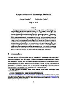
3-5 years. The interest rate associated with SBAs is the sum of the Special Drawing Rights (SDR) interest rate, margin, burden sharing adjustment, service fee, commitment fee and surcharges. • SDR interest rate is a weighted average of the 3-month U.S. T-bill rate, 3-month UK T-bill rate, Japanese Government 13-week financing bills, and 3-month Eurepo rate. • Margin is intended to cover the intermediation costs of the IMF and to help build reserves against credit risk. It is set at the beginning of every fiscal year by the management of the IMF. The average from May 1993-September 2008 is 62 bps and it is currently set at 100 bps.11 • A charge for burden sharing is added to cover losses resulting from over-due obligations to the IMF. These charges are refunded as overdue obligations are repaid. The average of the burden sharing adjustment from May 1986-September 2008 is 19 bps, and it is currently set at 2 bps. • A service fee of 50 bps applies to cover part of the intermediation costs and this fee is paid at the time the loan is disbursed. • A commitment fee is collected but refunded as the loans are withdrawn.12 This fee is 25 bps for loans up to the country’s quota, and 10 bps for those in excess of the quota. • In the case of SBAs, a surcharge of 100 bps apply to the portion of those loans that are greater than 200 percent of the country’s quota, and 200 bps for the portion greater than 300 percent. The sum of the SDR interest rate, margin, and burden sharing adjustment is called the adjusted rate of charge which is plotted in Figure 1 with historical averages reported in Table 1. Both in the table and the figure, the IMF’s adjusted rate of charge is compared with U.S. government bonds with 2, 3, and 5-year maturities since under SBAs, the loans are repaid within 3-5 years. The averages for the IMF’s adjusted rate of charge are in line with the yield on 3-year U.S. government bonds. This result is somewhat expected given that the SDR interest rate constitutes a significant portion of the adjusted rate of charge and the SDR rate itself is a weighted average of developed 11

The margin was negative for 1981-May 1993 since the rate of charge was not based on the SDR rate, and the imputed margin for that period is negative. 12 Therefore, commitment pertains to borrowing from the IMF rather than to repayment.

7

country T-bill rates with shorter maturities. Similarly, Jeanne and Zettelmeyer (2001) conclude that the IMF’s non-concessional lending rates, which include SBAs, are comparable to the risk-free rate. Note that the adjusted rate of charge and the above mentioned fees do not vary across countries. The only loan or country specific component of interest rates associated with SBAs is surcharges. These are determined by the size of the loan compared to the country’s quota but not by the riskiness of a sovereign. That said, there is an indirect channel through which the riskiness of a sovereign might impact the interest rate it faces upon borrowing from the IMF. The riskier the sovereign, or the more negative the output shock, the more it might borrow from the IMF thereby facing higher surcharges and interest rates. Another important feature of IMF lending is conditionality. IMF program-related conditions include macroeconomic and structural measures that fall under the core areas of the IMF’s expertise. According to IMF (2002a), these areas are “...macroeconomic stabilization, monetary, fiscal and exchange rate policies, including the underlying institutional arrangements and closely related structural measures, and financial system issues related to the functioning of both domestic and international financial markets.” IMF (2002b) reports that about 34 percent of the structural measures were related to the fiscal sector from 1994-1999 followed by the financial sector and privatization-related measures that constituted 16 and 14 percent of total measures, respectively. IMF conditionality is usually implemented using “performance criteria” that include performance targets on net international reserves, monetary policy, fiscal policy, and structural variables. The first one involves setting a floor for net international reserves. The second one typically includes a ceiling for net domestic assets of the Central Bank. The fiscal policy criteria consist of ceilings on overall balance and domestic financing of the deficit. It may also include limits to the size and level of external debt when indebtedness is considered to be an issue. Finally, structural performance criteria span a wide range of measures including financial sector reforms, privatization, etc. Inarguably, most of the aforementioned policies are aimed at containing aggregate demand. In our model this translates into a reduction in consumption. In addition, the fiscal contraction along with external debt performance criteria can be mapped into a reduction in the commercial debt stock of the sovereign. To understand whether our modelling of conditionality is consistent with these two, we calculate mean consumption and debt to the private sector in periods when the sovereign is indebted to the IFI but is not in default. In this setting it is important to exclude default periods since during default output falls (by assumption) and therefore consumption would 8

also fall. Similarly, since all the debt is forgiven after default, commercial debt stock would also decline dramatically. In order to abstract from these dynamics that are simply due to default per se, we focus on those periods with IFI borrowing but without default. Our model using the calibration elaborated in Section III implies that, consistent with the policies prescribed under conditionality, mean consumption during IFI borrowing periods is 6.5 percent lower than without IFI borrowing. Moreover, the mean commercial debt to GDP ratio falls by 13 percentage points of quarterly GDP. Using the available data on conditionality to conduct a comprehensive quantitative exercise or to quantitatively compare model implications with data is problematic because even when one focuses on the conditionalities related to fiscal policy, there is a wide variety of performance criteria and these criteria are often applied to different levels of government. For example, these criteria are applied to the central government budget in some countries, and to the general government in others. The aggregate that is used in most cases is the overall balance but there is a variation across countries in this regard as well with the use of extrabudgetary funds. This kind of heterogeneity makes it difficult to present meaningful cross country evidence on the quantity of adjustment that IMF programs involve.

2.2

Cyclical Properties

Although cyclical properties of commercial debt flows have been extensively studied in the literature, those of IMF lending have remained largely unexplored. In this section, we examine these properties for a set of emerging market economies and document our findings in Tables 3, 4, and 5. We choose the countries in our sample based on quarterly GDP data availability and on whether the country had an IMF program in the last two decades. Table 2 reports the main business cycle statistics associated with commercial debt for comparison. Table 2 establishes that commercial debt flows are procyclical, and highly variable. In addition, on average most sovereigns in our sample appear to be highly indebted to private sector creditors.13 Their standard deviations and correlations with the corresponding country’s real GDP are reported in the third and fourth columns of the Table, and the fifth column documents the mean commercial debt stock as a share of annual GDP. On average, the correlation of net lending by private sector creditors with real output is 0.37. This correlation is positive for all of the countries in the sample, lying between 0.14 (Peru) and 0.62 (Thailand and Turkey). The average standard deviation of this 13

Net debt flows by private sector creditors data reported in Table 2 are annual and are from the World Bank’s Global Development Finance Database (includes bonds, commercial banks, other debt to private creditors). Real GDP series are also from IFS. They are logged and HP filtered with smoothing parameter 100.

9

type of lending is 3.71 with Thailand being an outlier with a standard deviation of 10.10 percent. Finally, mean commercial debt stock is around 16 percent of annual GDP. Table 3 reveals that, IMF lending is countercyclical and has lower mean and variability than commercial lending. The countercyclicality of this type of lending with a correlation of -0.19 stands in contrast to lending by private sector creditors, which has a correlation of 0.37 with output.14 Countercyclicality holds for all countries except Thailand (0.26). The standard deviation of IMF debt flows reported in the third column of the same table suggests that IMF debt flows are remarkably less variable than commercial debt flows (0.82 vs 3.71). Comparing the debt ratios, the mean debt ratio to the IMF is lower than that to the private sector creditors (15.8 vs. 1.5 percent). Therefore, on average, IMF debt is around one tenth of private sector creditor debt. These results are in line with those of Ratha (2001) who finds that during 1996-1998, private flows to developing countries were 10-12 times multilateral flows. Table 4 reports statistics on the relationship between the use of IMF resources and country spreads based on J.P. Morgan’s EMBI Global spread data from Bloomberg. Since the first observation of spread data varies across countries, we report in the second column of the table, the periods considered in the calculations. The following two columns compare the average EMBI spreads for periods when there was positive use of IMF resources and those when the country was not using Fund resources. The number of observations are reported in parenthesis. Note that of the available sample of EMBI data, only Mexico and Thailand had a significant number of periods with and without use of Fund resources. For both of these countries spreads in periods with use of Fund credit are about three times the spreads in periods without Fund credit. All other countries were indebted to the IMF during a significant portion of the sample period. We find average spreads to be 617 (199) bps when Mexico (Thailand) was using Fund resources, while the average spreads were 242 (61) bps when it was not. Suspecting that the spread data might have outliers during crises, we also calculate median spreads and find these to be 488 (163) bps in periods when Mexico (Thailand) was indebted to the IMF versus 214 (58) bps when it was not. Finally, we compute the correlation between spreads and a dummy variable that is set equal to 1 when the country is indebted to the IMF. We find this correlation is positive for all countries in our sample with an average of 0.48.15 14

The finding, that in bust periods a country is more likely to have an IMF program, is not to say that one causes the other. Correlation does not imply causality. 15 Averages reported in the last row for E[s|d∗ > 0] and E[s|d∗ = 0] are weighted by the number of observations. The average for ρ(Id∗>0 , s) includes only those countries with at least four observations without use of Fund credit (Argentina, Brazil, Mexico, and Thailand).

10

These results on the relationship between spreads and IMF borrowing are roughly in line with those of Mody and Saravia (2006). Mody and Saravia (2006) find that spreads on bonds issued during an IMF program are higher. The authors collect data on launch spreads for more than 3,000 emerging market and developing country bonds and separate them based on whether they were issued during an IMF program or not. Their calculations reveal that the average spreads during IMF programs were 406 while they were 223 in the absence of programs. IMF borrowing is intermittent in that periods with borrowing are nested within periods without any borrowing from the IMF. This kind of pattern manifests itself as a higher standard deviation of net IMF flows than it would have been if borrowing from the IMF was more continuous. In addition to the standard deviations already reported in Table 3, we also calculate the probability of positive use of IMF resources from its GRA account (P r[d∗ > 0]) to get a sense of the frequency of IMF borrowing. Table 5 documents that the unconditional probability of having a program with the IMF is 46 percent for 1945-2007 and 55 percent for 1970-2007 when we expand our sample to 17 emerging market economies. The rationale for expanding our sample for this exercise is to get a more unbiased picture because one of our selection criteria for the initial sample was to include countries with significant IMF borrowing in the last several decades. So by construction, the probability of the use of IMF credit would be biased upwards. The additional countries included in the calculation of the mean reported in the last row of Table 5 are Chile, Colombia, Egypt, India, Korea, Malaysia, Singapore, and Venezuela. Note that these probabilities are higher for our original sample with 9 countries.16 Table 5 reveals that countries are more likely to be indebted to the IMF when output is below trend. The second and third columns of Table 5 report the unconditional probabilities and probabilities conditional on output being below trend, respectively.17 Subtracting the third column from the second yields probabilities conditional on output being above trend. On average, the probability of having an IMF program when output is low is greater (30 percent) than when output is high (25 percent). This holds for all countries in our sample except Argentina. Note that the probability of borrowing from the IMF is significant even when output is above trend. One potential reason for this could be that most emerging markets recover relatively quickly after a crises. If a country 16

Barro and Lee (2005) calculate the fraction of time that a country had an IMF program (SBA or EEF) to be 0.185 using data for 130 countries from 1975-1999. They also calculate IMF loan approval frequency to be 0.364. Approval frequency is calculated by assigning ‘1’ if the country had a loan approved within a 5-year interval. Our numbers differ from theirs mainly because we focus only on large emerging market economies and also our dummy is based on quarterly data rather than 5-year intervals. 17 We restrict our analysis to a shorter sample in these two columns because real GDP series become available for all countries starting in 1967.

11

gets an IMF loan during crisis and output bounces back quickly before the repayments to the IMF are complete then the country can be considered a user of IMF resources while its output would have already recovered. Another difference between IFI debt and commercial debt pertains to repayment history. According to Reinhart, Rogoff and Savastano (2003), all countries in our sample have defaulted at least once on their external commercial debt with the exception of Thailand. In contrast, essentially all IMF loans to major emerging market economies have always been repaid. Zettelmeyer (2005) writes: “In the past, the IMF has virtually always been repaid, but this leaves the possibility that currently open lending relationships may eventually result in arrears or debt forgiveness.” Jeanne and Zettelmeyer (2001) find that “most open lending relationships with emerging market countries are statistically similar to past lending cycles that eventually ended in repayment while the very long open lending cycles of many poor countries statistically ‘look’ like they might continue forever.” Similarly, Eichengreen (2003) and Saravia (2004) argue that the IMF loans are typically repaid. Only during the debt crises of the 1980s was there an increase in non-repayment cases. According to Zettelmeyer (2005), there were thirteen countries in protracted arrears to the IMF.18 However, most of these countries have repaid, and in particular the only emerging market among these countries, Peru, has repaid. To summarize, this section establishes that: • The IMF lending rate under SBAs can be approximated by the sum of the risk free rate and a charge that increases with the amount borrowed. • Lending by private sector creditors is procyclical whereas IMF lending is countercyclical. • Debt to the private sector creditors is about four times more variable than that to the IMF. • The average debt stock to the IMF is about one tenth of the debt to private sector creditors. • Country spreads are higher in periods when countries are indebted to the IMF. • The unconditional probability of the use of IMF resources is about 50 percent for emerging markets. • The IMF has almost always been repaid, particularly by emerging market economies. 18

Cambodia, Guyana, Haiti, Honduras, Liberia, Panama, Peru, Sierra Leone, Somalia, Sudan, Vietnam, Zaire, and Zambia.

12

3

Model

The model features competitive, risk-neutral private sector creditors, an IFI, and a sovereign that maximizes the utility of its households. The model mainly builds on the work of Eaton and Gersovitz (1981) on sovereign debt with potential repudiation. The distinguishing and appealing feature of this framework is the lack of commitment of the sovereign to repay its debt to the private sector creditors. Due to this commitment problem, the sovereign may optimally default on its debt to this type of creditors. Therefore, this model analyzes a “willingness to pay” scenario rather than “ability to pay.” Every period the sovereign is in one of two states: default or non-default vis-a-vis the private sector creditors, D, N . Starting in the non-default state, the sovereign has access to borrowing commercially. In these non-default states, the sovereign observes its output level, makes a decision on whether to default or not, and also whether to borrow from the IFI. If it chooses to default, it does not repay its existing debt, but as a punishment, it loses access to commercial borrowing for a period with exogenously and stochastically determined length. If it does not default, however, it repays its debt obligations in full, chooses how much to borrow commercially and from the IFI, and maintains the option to default in the following period. During exclusion from commercial borrowing, the sovereign only chooses whether to borrow from the IFI based on its remaining output after incurring losses due to default. The IFI lends to the sovereign at the risk-free rate plus a debt elastic component intended to capture the surcharges of the IMF.19 The sovereign does not face a commitment problem in repaying its debt to the IFI because of the preferred creditor status of the IMF and also the observation that major emerging market economies have almost always repaid their debt to the IMF. There is only one IFI with a non-profit role as an international financial institution in this context. In our setup, the existence of the IFI provides the sovereign with an additional instrument to smooth consumption that is available even during exclusion from commercial credit markets. Borrowing from the IFI is preferable in times when the default probability on private sector debt is high (and as a result the interest rate is high) or when the sovereign is in default and does not have access to commercial credit markets at all. 19

As discussed in Section 2, the rate applied by the IMF includes a surcharge determined by the amount borrowed.

13

The sovereign makes its default decision in the following fashion: V (d, d∗ , y) = max{V D (d∗ , y), V N (d, d∗ , y)} D

(1)

where D is the binary variable that represents the decision to default (D = 1) or not (D = 0), y is output as explained below, and d and d∗ denote the debt stock to private sector creditors and the IFI, respectively. Note that the value of default, V D , depends on output and IFI debt because the level of commercial debt becomes irrelevant when it is not repaid. However, the value of non-default, V N , and the decision on whether to default or not, D, depend on the level of debt to IFI and commercial debt as well as output. Default, D = 1, is chosen if and only if V D > V N . For state (d∗ , y) the value of default can be expressed as: V D (d∗ , y) = max {u(c) + β(d∗0 ) ∗0 d

X£

¤ θV (0, d∗0 , y 0 ) + (1 − θ)V D (d∗0 , y 0 ) π(y 0 |y)}

(2)

y0

where u is CRRA per-period utility, u(c) =

c1−σ 1−σ ,

c is consumption, and β(d∗0 ) is the discount

factor elaborated further below.20 An implicit assumption in this formulation is that once the country regains access to commercial borrowing, all of its commercial debt is forgiven and it starts with d = 0. θ is the exogenously determined probability of entry to the credit market after default; therefore, it gives the average duration of exclusion once the sovereign defaults. The budget constraint during exclusion is y def = c + d∗ − q ∗ d∗0

(3)

where q ∗ is the price of IFI debt which can be written as: q ∗ (d∗0 ) =

1 . 1 + r + φ(d∗0 )

(4)

Note that this price depends only on d∗0 and not on d0 or y. Output is exogenous and is characterized by an AR(1) process: y = ez 20

Throughout the paper, primes refer to the following period.

14

(5)

where zt = ρzt−1 + ²t and ² ∼ N (0, σz2 ). We approximate this Normal process with a Markov chain with S states and transition probability matrix π. π(yj |yi ) denotes the probability of transiting from state i to j. The output process is truncated during default as in Arellano (2008) in order to bring the default probability implied by the model in line with those in the data. We assume that the direct output cost of default increases with output. In other words, if a country defaults when its output is high, the output loss due to the default decision would be higher as opposed to a sovereign that defaults when its output is low. Mathematically:

y def

  y, if y < yˆ =  yˆ, if y > yˆ.

In non-default periods, the sovereign decides whether or not to default, and how to allocate its financing needs among the private sector creditors and the IFI. The value of non-default in this setup can be written as: V N (d, d∗ , y) = max {u(c) + β(d∗0 ) 0 ∗0 d ,d

X

V (d0 , d∗0 , y)π(y 0 |y)}

(6)

y0

subject to the budget constraint: c = y − d + qd0 − d∗ + q ∗ d∗0 .

(7)

As mentioned above, the risk neutral and perfectly competitive private sector creditors lend at a rate that is mainly determined by the default probability of the sovereign. The commercial bond price schedule is given by: q(d0 , d∗0 , y) =

1 − E[λ(d0 , d∗0 , y)] 1+r

(8)

where λ(d0 , d∗0 , y) = P rob[V D (d∗ , y) > V N (d, d∗ , y)] captures the default probability and the spread is defined as s = 1/q − 1 − r. In order to capture the conditionality of IMF loans, and also to account for the regularity that sovereigns do not borrow from the IMF every period as documented in Table 5, we assume that the sovereign has to switch to a higher discount factor (that is, a lower discount rate) as long as it is indebted to the IFI. Models of sovereign default have traditionally calibrated discount rates so that they are significantly greater than the risk free interest rate. In this fashion, more realistic debt 15

ratios and default probabilities are achieved because, with a low discount factor, the sovereign has a strong desire to consume today and is willing to hold larger amounts of debt in the long run. By assuming that borrowing from the IFI is associated with a higher discount factor, we are building “more prudent” policies that come with conditionality. This can also be interpreted as a reduction in consumption (public consumption in particular) that typically is part of conditionality. More formally:

  β H , if d∗0 > 0 β(d∗0 ) =  β L , if d∗0 = 0.

The recursive equilibrium of this economy is characterized by price schedules for commercial debt, q(d0 , d∗0 , y) and official debt, q ∗ (d∗0 ), debt and consumption allocations , d0 (d, d∗ , y), d∗0 (d, d∗ , y), and c(d, d∗ , y) such that: 1. The sovereign maximizes its utility subject to the budget constraint taking the price schedules as given. 2. Given the default probabilities implied by the debt position and output of the sovereign, private sector creditors lend at price q(d0 , d∗0 , y) and break even in expected value while the IFI lends at q ∗ (d∗0 ) to the sovereign. 3. The goods market clears.

4

Quantitative Analysis

4.1

Calibration and Data

We have three sets of parameters, those borrowed from the sovereign debt literature, those estimated from the data and those calibrated to match certain model statistics to the data. All parameters are reported in Table 6. The risk aversion coefficient and risk-free rate are standard both in the sovereign debt and small open economy business cycle literatures which are set to 2 and 1%, respectively. Following Arellano (2008) and Aguiar and Gopinath (2006), we set the probability of redemption to 10 percent, implying an average exclusion of 10 periods (2.5 years with quarterly calibration). We estimate the parameters governing the output process using quarterly Argentine GDP data for the two decades before its default (1980Q1-2000Q4) obtained from Neumeyer and Perri (2005).21 21

Similarly, we report model statistics after excluding default episodes to make them comparable with the data. However, for those statistics regarding borrowing from the IFI, we include the default periods both in the data and in the model. This is to capture IFI borrowing dynamics during default as well.

16

The GDP series is deseasonalized, logged and HP filtered with smoothing parameter 1600. With our notation of y = ez where zt = ρzt−1 + ²t and ² ∼ N (0, σz2 ), we estimate an AR(1) process and find ρ = 0.91 and σz = 0.019. Using these AR(1) parameters, we estimate a Markov process with nine states using Tauchen’s algorithm. We assume φ(d∗ ) = kd∗ for simplicity. As a result, we have four parameters remaining that need to be calibrated: yˆ, k, β L , and β H . These parameters are calibrated to match four model moments: number of defaults, mean public debt to commercial debt ratio (E[d∗ ]A /E[d]A ), the standard deviation of IFI flows (σ(∆d∗ /y)), and mean IFI spread (E[s∗ ]). The values obtained as a result of this calibration exercise are reported in Table 6. Argentine business cycle statistics are reported in the first column of Table 7. We use the same series on private sector creditor debt and IMF lending as in Section 2 except that we utilize quarterly IMF lending data available in International Financial Statistics as our model calibration is quarterly. Since private sector creditor debt data is annual, simulated data related to borrowing from private sector creditors are also annualized to facilitate comparison. The number of defaults is calculated based on Reinhart, Rogoff, and Savastano (2003) who report that Argentina defaulted four times in the period 1824-1999. Adding the most recent default episode in 2001, we have five defaults in 186 years which translates into 67.2 defaults per 10,000 quarters.

4.2

Findings

Existing sovereign debt models with only private sector creditors establish that a high level of debt strengthens the incentive to default because the gain from default is the amount of debt that is forgiven.22 Conversely, a high output realization strengthens repayment incentives as the sovereign can afford to repay without facing low levels of consumption. As a consequence, these models imply countercyclical interest rates in line with the emerging markets data. This prediction of countercyclical interest rates is in fact one of the distinguishing features of the last generation of sovereign debt models with incomplete markets from those under complete markets that imply procyclical interest rates.23 These features are present in our two creditor setup as well as those that arise due to the introduction of the IFI discussed below. The default probability on commercial debt increases with the level of IFI debt although not as fast as it does with commercial debt. This is evident in the commercial debt price schedule 22

See Arellano (2008), and Aguiar and Gopinath (2006) for a discussion of the equilibrium, solution and implications of models with one type of creditor. 23 See Kehoe and Levine (1993) and Alvarez and Jermann (2000).

17

plotted in the top panel of Figure 2. This pricing schedule is steep suggesting that small increases in d0 increase interest rates significantly; however, the interest rate difference between high and low levels of d∗0 is not large. The steepness is intuitive given that commercial debt is directly linked to the benefit of default. For the case of IFI debt, there are two effects working in opposite directions. First, since IFI debt is not defaultable, a high level of it implies a higher IFI debt service in the following period leaving the sovereign with less resources to repay commercial debt. This channel suggests that the higher the IFI debt, the higher the default probability on commercial debt. Second, positive IFI debt forces the sovereign to discount the future less and act more prudently lowering default probabilities. As suggested by Figure 2, ceteris paribus the first effect is quantitatively larger leading to commercial interest rates that increase with IFI debt in equilibrium. An implication of Figure 2 is that a shift in sovereign’s portfolio towards IFI debt in response to a negative output shock does not suffice to reduce spreads.24 As mentioned above, any type of debt, official or commercial, leads to higher interest rates. However, the interest rates are much more elastic with respect to commercial debt than IFI debt. Given a certain level of total debt, a portfolio with only commercial debt leads to higher spreads than one that includes any IFI debt. The model performs well in matching the non-target moments. Those moments related to IFI borrowing that are not used in the calibration exercise are the correlation of IFI debt flows with output, ρ(∆d∗ /y, y), the correlation of IFI debt dummy with spreads, ρ(Id∗ >0 , s), and the frequency of borrowing from the IFI, P rob(d∗ > 0). In addition to the model doing a good job in matching these statistics (perhaps with the exception of the frequency of IFI borrowing that appear to be lower in the model than compared to the data), it matches well those statistics related to commercial debt flows. The weak countercyclicality of IFI debt is due to the decoupling of the interest rate charged by the IFI from default probability, which is an implication of enforceability of IFI debt contracts. Countercyclical debt flows are a prediction of canonical SOE-RBC models that assume enforceable debt contracts. In those models, as a result of the consumption smoothing motive, agents choose to save in good times and borrow in bad times, hence countercyclical flows. Our framework in some sense synthesizes these strands of models by introducing enforceable and non-enforceable contracts into a unified framework. Our framework that incorporates both enforceable and nonenforceable contracts nicely preserves the cyclical properties of each type of debt flow established 24 This is not to say that the existence of the IFI leads to higher spreads. We conjecture that spreads would have been even higher in absence of IFI borrowing and portfolio reallocation of the sovereign.

18

in the literature. The sovereign makes debt allocation decisions in non-default periods by comparing the cost of borrowing commercially and the cost of IFI debt. The cost of borrowing commercially increases when the economy is hit by a negative output shock. However, the cost associated with IFI debt depends on the realizations of these shocks only indirectly through their impact on d∗0 . As a result, the sovereign chooses to hold less commercial and more official debt in its portfolio in bad times, (ρ(∆d/y, y) = 0.28, ρ(∆d∗ /y, y) = −0.08). The model performs particularly well in matching the correlation between the Fund credit use dummy and spreads (0.22 in the data vs 0.25 in the model). In addition, in the model, spreads in periods with positive IFI debt are 2.46 times those with no IFI debt. This is in line with the data documented in Section 2. For Mexico and Thailand, this ratio is 2.55 and 3.25, respectively. For Argentina, E[s|d∗ > 0] is as high as 2100 bps, which is driven by a few outliers in the data. For this country, the ratio of median spreads conditional on being and not being indebted to the IMF is 2.32, remarkably close to the result generated by the model. The intermittency of borrowing from the IFI is evident in P r(d∗ > 0) in Table 7. Introduction of two different discount factors generates a fixed cost-like effect making it possible for the model to account for intermittent IFI borrowing. When output is high, the sovereign prefers d∗ = 0 keeping the discount factor low. However, when output is low, the sovereign chooses relatively higher values of d∗ . Therefore, small but positive values for d∗ are almost never optimal. These dynamics allow us to match the lumpiness and probability of use of Fund credit in the data. To ensure that these fixed cost-like effects are in fact due to the introduction of two different discount factors, we strip out the other ingredients of the model and analyze a simple small open economy consumption-savings setting explained in the Appendix. The aforementioned effect is present in that simple model, confirming our intuition. The sovereign in our model borrows from the IFI with a 34 percent probability. This is fairly close the average borrowing probability of 46 percent reported in Table 4. In terms of spreads, we used the mean IFI spread, E[s∗ ], as a target moment. Mean commercial debt spread, E[s], implied by our model is 2.75, substantially higher than the mean IFI spread. In the data, mean commercial debt spreads are as high as 7.08 percent. Unfortunately, the sovereign default models have difficulty in generating the high level of spreads that we see in the data, mainly because the spreads are determined in equilibrium by risk neutral pricing using the default probabilities. (See Arellano (2008) for a discussion.) Our model does not provide an improvement 19

in this regard. Similarly, the introduction of an IFI does not help reduce the discrepancy between the level of commercial debt in the model and in the data, another shortcoming established in the literature. To further compare model implications with the data, we analyze the behavior of IFI debt in high and low spread periods. Table 8 reports average IFI debt when spreads are above the 75th percentile, below the 25th percentile, and when the sovereign is in default. This exercise allows us to assess model performance in yet another dimension not captured by the business cycle statistics. The model generates a mean IFI debt stock of 2.76 (2.39) percent when spreads are high (low). These are lower than those implied by the data, 7.83 (8.23).25 However, note that the difference in mean IFI debt between high and low spreads is close to the data. Average IFI debt during default is 26.74 percent in the model, remarkably close to that in the data (31.87).26 Finally, we conduct a similar exercise looking at the mean IFI debt during booms and busts defined as periods when endowment falls at least one standard deviation and periods when it exceeds its mean by at least one standard deviation. The model matches the qualitative features of the data by generating a mean IFI debt during busts (5.50) that is higher than that during booms (0.06). In the data, these mean IFI debts are higher than those implied by the model with 9.23 percent during busts and 7.43 percent during booms.

4.3

Sensitivity Analysis

Our sensitivity analysis focuses on the parameters that govern the cost of IFI borrowing, which we could not estimate from the data. In Table 10, we present five sets of results with different levels of conditionality and values for k, the parameter governing the elasticity of the IFI interest rate with respect to the level of IFI debt. In this subsection, we compare the first four scenarios to the baseline and find that our main results (weak countercyclicality of IFI debt flows and higher spreads when indebted to the IFI) are by and large robust. The fifth scenario is discussed in the next subsection. The first column of Table 10 reproduces the results with baseline parametrization to facilitate comparison. The second column reports those with no conditionality, that is β H = β L = 0.97. Without conditionality, the average official debt holdings increase from 3.09 to 6.02 with frequency 25

This discrepancy is largely due to our calibration strategy of matching E[d∗ ]/E[d] to data as opposed to E[d∗ ] which leads to lower levels of IFI debt generated by the model. 26 Calculating similar statistics for commercial debt was not possible because of short time series data on spreads at annual frequency and commercial debt data is annual.

20

of d∗ > 0 increasing from 34 percent to 98 percent. Mean IFI debt spreads go up proportionally to E[d∗ ]. The other statistics do not change significantly except ρ(Id∗ >0 , s) and σ(∆d∗ /y). The result that IFI debt is chosen to avoid high levels of interest rates somewhat strengthens and the countercyclicality increases marginally. Without the fixed cost of IFI borrowing, the sovereign can more effectively utilize this instrument in bad times to avoid high interest rates and low consumption levels. When IFI lending has no conditionality, we find that the sovereign still borrows more commercially than from the IFI. A priori one might expect the opposite, i.e., the sovereign would borrow more from the IFI considering that the mean spreads are lower for the IFI than the commercial debt. Despite higher spreads associated with commercial debt, it has an important advantage over IFI debt in that it is defaultable. The E[d∗ ]A /E[d]A ratio increases from 0.24 in the baseline to 0.47 in the no conditionality scenario revealing that the sovereign chooses to hold a significantly higher IFI debt in proportion to commercial debt. However, this ratio does not reach one for the aforementioned reason. The higher conditionality scenario reported in the third column largely works in the opposite direction compared to the no conditionality scenario. The average IFI debt levels and frequency of IFI borrowing are lower. This scenario implies lower number of defaults (43 vs 64 in the baseline) and consistently lower mean commercial debt spreads. The standard deviation of IFI debt flows fall along with its mean mainly because 96 percent of the time, the sovereign does not borrow at all from the IFI lowering both mean and variability of this type of debt. The ability of the sovereign to use IFI debt to avoid high commercial interest rates disappears in this case evidenced by a weak negative correlation between the IFI debt dummy and spreads. Reducing k to 0.165 from 0.175 in the baseline causes average IFI debt and frequency of IFI borrowing to be higher than the baseline. This is expected considering that k determines the spreads of IFI debt over the risk free rate for a given level of d∗ . All other results remain more or less similar to the baseline with somewhat higher variability of IFI debt and commercial debt spreads that appear to go hand in hand in our simulations. Note that mean IFI debt spreads are higher in this case despite k being lower because higher mean IFI debt more than offsets a potential decline in the spreads due to lower k. The fifth column of Table 10 reports the statistics of the scenario with a higher k. Contrary to the lower k scenario, this scenario reduces average IFI debt and its frequency. The high k scenario leads to lower IFI debt holdings as well as a smoother pattern for its flows. Mean IFI debt spreads 21

fall in this case because of the significant decline in mean IFI debt. The weak countercyclicality result survives in all of the cases we examine in our sensitivity analysis suggesting that this result is mainly related to IFI debt being nondefaultable which leads to the inelasticity of the IFI interest rate to output shocks and to the level of commercial debt. Finally, not reported in Table 10, is an experiment we conducted assuming no IFI conditionality and no surcharges, i.e., β H = β L = 0.97 and k = 0. The sovereign therefore has to allocate its portfolio between a defaultable bond where the interest rate is determined by the default risk and a non-defaultable bond with interest rate the same as the risk-free rate. We find low mean commercial debt, but nonzero, high frequency of default coupled with high mean commercial debt spreads. These findings imply that the sovereign rarely borrows commercially and whenever it does, it ends up defaulting on it. The weak countercyclicality of IFI debt is also robust in this case confirming that the key feature of the debt driving this result is its being non-defaultable.

4.4

Role of IFI Lending

Having set up a model that captures key characteristics of IFI lending, in this section, we further explore the role played by IFI lending. To do so, first, we look at the model moments when loans from the IFI are unavailable. We achieve this by setting both k and β H to high values such that effectively borrowing from the IFI is not an option. Second, we conduct welfare analysis. Model moments without IFI lending are reported in the last column of Table 10. Comparison of these results with those from our baseline model with IFI lending delivers mixed results as to whether the sovereign is better off when borrowing from the IFI is possible. Consumption variability to output variability ratio and consumption’s correlation with output are unchanged across these two scenarios. When borrowing from the IFI is not possible, the mean total (both private and IFI) debt stock of the sovereign is higher and at the same time, default is less frequent and hence the spreads on private sector debt lower. The sovereign has more incentives to repay commercial debt in this case since default implies autarky leaving the sovereign without any instruments through which consumption can be smoothed. From a narrow perspective, the presence of IFI debt does not help complete markets since it is not a contingent contract paying only on certain exogenous states of nature, i.e. endowment shocks. However, the price function associated with it is contingent on only part of the state space (including endogenous and exogenous state variables) unlike that of private sector creditor debt which is contingent on the entire state space. In other words, q ∗ (d∗0 ) while q(d0 , d∗0 , y). It has 22

different terms from private sector creditor debt and therefore does provide the sovereign with a non-redundant instrument. A priori it is difficult to conjecture whether IFI lending would improve or reduce sovereign’s welfare. At a first glance one may be tempted to think that IFI lending is another instrument provided to the sovereign that can potentially facilitate better transfer of wealth over time, and it cannot make it worse off since the sovereign can always choose not to borrow from the IFI. This logic would hold in an environment without frictions where competitive equilibrium allocations are necessarily Pareto efficient. However, our setup incorporates limited commitment and incomplete markets that imply a deviation from the assumptions of the first fundamental theorem of welfare economics. The closest study from the literature that examines efficiency in a limited commitment framework is Zame (1993). He shows that opening new markets for securities does not necessarily improve efficiency if these securities are non-defaultable. He argues, however, that making default an option may improve efficiency by allowing the debtor not to pursue repayment in states when debt exceeds income. Based on this argument, the presence of IFI debt, which in some sense is opening a new securities market, may not improve efficiency as it is non-defaultable. Given the mixed results based on model moments and the limited help from the literature on this issue, we proceed numerically to evaluate the impact of IFI lending on the welfare of the sovereign. Our measure of welfare is compensating variations in consumption that equate expected lifetime utility in the baseline model with that of the setup without IFI lending. More formally, we solve for g in the equation g 1−σ V IF I (d, d∗ , y) = V no−IF I (d, d∗ , y) and evaluate its expected value where V IF I and V no−IF I denote the value functions of the scenarios with and without the IFI, respectively. We find that, as it is modelled, the presence of IFI lending, on average, leads to a welfare decline of 0.34 percent in units of consumption. A state by state comparison suggests that conditional on the sovereign being highly indebted to the private sector creditors and output being low, the baseline scenario with the IFI yields higher welfare than the one in which IFI lending is non-existent. In fact, for the lowest realization of output and highest level of commercial debt, the improvement in welfare in the baseline scenario reaches about 1 percent as plotted in Figure 3. With this realization of output, the improvement in welfare declines monotonically to -0.75 percent, a reduction in welfare, as commercial debt falls. In the case of the highest output realization, the sovereign’s welfare declines in the baseline compared to when there is no-IFI lending. 23

Note that in our setting we did not incorporate any output improvement that IFI lending and its conditionality could provide to the sovereign. There is no investment or capital accumulation, and as a result, the foregone consumption in the current period can reduce future debt but does not improve dynamics of future output which are determined by an exogenous process. In this paper we do not empirically estimate the impact of IFI lending on output but argue that a 0.34 percent improvement in output is a relatively small number. It is plausible that most of the benefits of IMF programs can be reaped in the long-term well after the program is over, especially if the program involves structural measures as argued by Ghosh et. al (2005) and Faruqe and Khan (2002).

5

Conclusion

This paper proposed a framework for analyzing dynamics of lending by IFIs in international credit markets. This framework sheds light on the decisions of a sovereign borrower regarding when to default on its commercial debt in the existence of an IFI and how to allocate its borrowing needs among these two types of creditors. Differences in the contracts offered by private sector creditors and IFIs take us a long way in accounting for the stark differences in cyclical properties of these two types of debt. Characteristics of IFI lending are modelled based on the institutional framework of the IMF’s Stand-By Agreements. The interest rate charged does not depend on the sovereign’s riskiness but only on the size of the loan. In addition, as long as the sovereign is indebted to the IFI, it has to follow more prudent policies, modelled as the sovereign acting as if it had a higher discount factor, valuing future consumption more than it would without any IFI debt. The model successfully accounts for the weak countercyclicality of IFI debt flows as well as the fact that IFI debt stock tends to be higher in times of high spreads. These findings are shown to be robust to the key parameters. Moreover, we conclude that conditionality plays a key role in intermittency of borrowing from the IFI while enforceability of IFI debt contracts explains its relatively small size and countercyclicality observed in the data. The recent increase in demand for IMF loans by emerging market economies underscores the importance of understanding the dynamics of IMF lending, or more generally, IFI lending and its impact on a sovereigns’ decisions. In addition to providing a setting that accounts for key regularities in the data, the model laid out in this paper can be utilized to answer policy questions regarding the design of IMF lending facilities. The current setting mimics SBAs, however, one

24

could model other facilities such as the new flexible credit line and compare its implications on debt and default.

25

Appendix: Solution In this setting with two types of creditors, the sovereign not only makes default d ecisions but also faces a portfolio allocation problem in non-default periods. Depending on the realizations of output and its current level of debt to each type of creditor, the sovereign allocates its borrowing needs. Given that these creditors lend with different terms, we can solve the sovereign’s portfolio choice problem using standard techniques explained below. Initially, we solve for the competitive equilibrium of the model with state spaces of d and d∗ spanning a wide interval. We find that commercial debt has a well-defined stationary distribution in the interval [0.02, 0.34] and d = 0 is imposed in default periods. This reveals that any commercial debt level in the (0, 0.02) range is not optimal. We use this observation to “economize” on the nodes. We place (N B − 1) equally spaced nodes in the [0.02, 0.34] interval, {d1 , d2 , d3 , ..., dN B−1 } ∈ [0.02, 0.34] and concatenate them with {dN B } = {0}. The ergodic distribution of IFI debt also displays such discontinuity, however; it is not as strong as the one for commercial debt. Therefore, we set the state space for d∗ to span the interval [0, 0.36].27 In order to find the equilibrium allocations and price schedule for private sector debt, we implement the following algorithm: 1. Discretize the state space as explained above. 2. Conjecture a price schedule for private sector debt, q old (d0 , d∗0 , y) =

1 1+r .

3. Solve the sovereign’s problem recursively using value function iteration by taking the conjectured price schedule for private sector debt and IFI debt price schedule as given and obtain default decisions D(d, d∗ , y), policy functions d0 (d, d∗ , y), d∗0 (d, d∗ , y), and c(d, d∗ , y). 4. Given these policy functions, calculate default probability λ(d0 , d∗0 , y). 5. Using the default probability λ(d0 , d∗0 , y), calculate a new price schedule, q new (d0 , d∗0 , y) = 1−E[λ(d0 ,d∗0 ,y)] . 1+r

6. Update the conjectured price schedule q old (d0 , d∗0 , y) with a weighted average of q old (d0 , d∗0 , y) and q new (d0 , d∗0 , y). Repeat these steps until convergence is obtained, that is, max |q old (d0 , d∗0 , y)− 27 Note that by limiting the lower limit of IFI debt to zero, we assume that the sovereign cannot lend to the IFI. In practice, some countries in particular advanced economies can be creditors to the IMF. With our calibration, even if the sovereign is allowed to be a creditor, it would never choose to do so in the model. We consider this a plausible scenario given our focus on emerging market economies.

26

q old (d0 , d∗0 , y)| < ξ where ξ is a very small number.28 Note that Hatchondo, Martinez, and Sapriza (2007) need to keep track of the government type as a state variable and evaluate different continuation values for different types. In our setting, sovereign essentially chooses its own type and the information with regards to its type can be inferred from its debt to the IFI making it unnecessary to include it as a separate state variable.

Appendix: Simple Small Open Economy Model In this section we analyze a simple small open economy model to elaborate further the implications of switching to a higher discount factor when in debt. We solve the following model with a constant interest rate assuming that commitment technology exists, so there is no default. In order to simplify the analysis further and increase the accuracy of the results, we assume there is only one lender that lends at the risk free rate. However, whenever the country borrows from this creditor, it has to switch to a higher discount factor. Similar to our benchmark model, we assume an endowment economy but with an i.i.d. exogenous stochastic process. More formally, the small open economy would solve: max E0 ct

∞ X

β(bt+1 )t u(ct )

t=0

subject to ct + bt+1 = yt + bt (1 + r)

(9)

b denotes bond holdings, y is endowment, and interest rate r is assumed to be constant. We assume a CRRA utility function and set β(1 + r) < 1 to ensure stationarity for bonds. This is a standard consumption-saving problem in the case of a small open economy except that the lender requires the economy to switch to a different discount factor as a condition for lending:   β H , if b < 0 β(b) =  β L , if b = 0. This specification for the discount factor is the same as that in our benchmark two creditor model with default. Figure 4 plots the stationary distributions for two parameterizations of this model, a baseline 28

Note that the calculation of q ∗ does not require solving for a fixed point. For given φ(d∗0 ), we can evaluate q ∗ (d∗0 ) and plug in the budget constraint of the sovereign.

27

parameterization with β H = β L = 0.98 and one with different discount factors β H = 0.98, β L = 0.979965. All other parameters are kept the same with the standard deviation of output set to 4.5 percent. We set β L such that b0 < 0 is chosen around 60 percent of the time, again similar to our benchmark model. We find that one needs to set β H − β L to a very low number in order to obtain the 60 percent probability of a negative bond position. Larger differences between the two discount factors quickly lead to the country choosing autarky as opposed to borrowing and switching to a higher discount factor. This is likely to be a result of the fact that in these models the welfare cost of living in autarky is small. Having to switch to a higher discount factor leads the country not to choose negative but small (in absolute value) bond positions. Instead of borrowing a small amount, it becomes optimal not to borrow at all and stay in the low discount factor. This is evident in Figure 4 which reveals that bond positions in the interval [−0.04, 0] are almost never chosen.

28

References [1] Aguiar, Mark and Gita Gopinath, 2006, “Defaultable Debt, Interest Rates and the Current Account,” Journal of International Economics, vol. 69, pp. 64-83. [2] Alfaro, Laura and Fabio Kanczuk, 2005, “Sovereign Debt as a Contingent Claim: A Quantitative Approach,” Journal of International Economics, vol. 65, pp. 297-314. [3] Alfaro, Laura and Fabio Kanczuk, 2007, “Optimal Reserve Management and Sovereign Debt,” Harvard Business School working paper, No. 07-010. [4] Arellano, Cristina, 2008, “Default Risk, the Real Exchange Rate and Income Fluctuations in Emerging Economies,” American Economic Review, vol. 98, pp. 690-712. [5] Arellano, Cristina and Ananth Ramanarayanan, 2008, “Default and the Term Structure in Sovereign Bonds,” University of Minnesota mimeo. [6] Bai, Yan and Jing Zhang, 2005, “Financial Integration and International Risk Sharing,” University of Minnesota mimeo. [7] Barro, Robert J. and Jong-Wha Lee, 2005, “IMF Programs: Who is Chosen and What are the Effects?,” Journal of Monetary Economics, 52, pp. 1245-1269. [8] Cole, Harold , James Dow, and William B. English, 1995, “Default, Settlement and Signalling: Lending Resumption in a Reputational Model of Sovereign Debt,” International Economic Review, 36, pp. 365-385. [9] Corsetti, Giancarlo, Bernardo Guimaraes, and Nouriel Roubini, 2006, “International Lending of Last Resort and Moral Hazard: A Model of IMF’s Catalytic Finance,” Journal of Monetary Economics, 53, pp. 441-471. [10] Cottarelli, Carlo and Curzio Giannini, 2002, “Bedfellows, Hostages, or Perfect Strangers? Global Capital Markets and the Catalytic Effect of IMF Crisis Lending,” IMF Working Paper No. 02/193. [11] D’Erasmo, Pablo, 2008, “Government Reputation and Debt Repayment in Emerging Economies,” University of Maryland mimeo.

29

[12] Eaton, Jonathan and Mark Gersovitz, 1981, “Debt with Potential Repudiation,” Review of Economic Studies, vol. 48, pp. 289-309. [13] Eichengreen, Barry, 2003, “Restructuring Sovereign Debt,” Journal of Economic Perspectives, vol. 17, pp.75-98. [14] Eichengreen, Barry, Poonam Gupta, and Ashoka Mody, 2006, “Sudden Stops and IMFSupported Programs,” NBER Working Paper No. 12235. [15] Ghosh, A., T. Lane, M. Shulze-Ghattas, A. Bulir, J. Hamman, and A. Mourmouras, 2002, “IMF Supported Programs and Capital Account Crises,” IMF Occasional Paper No. 210. [16] Ghosh, A., C. Christofides, J. Kim, L. Papi, U. Ramakrishnan, A. Thomas and J. Zalduendo, 2005, “The Design of IMF-Supported Programs,” IMF Occasional Paper No. 241. [17] Guimaraes, Bernardo, 2006, “Optimal External Debt and Default,” London School of Economics mimeo. [18] Haque, Nadeem and Mohsin S. Khan, 2002, “Do IMF-Supported Programs Work? A Survey of the Cross-Country Empirical Evidence,” Macroeconomc Management: Programs and Policies, pp. 38-57. [19] Hatchondo, Juan Carlos, Leonardo Martinez and Horacio Sapriza, 2007, “Heterogeneous Borrowers in Quantitative Models of Sovereign Default,” International Economic Review, forthcoming. [20] International Monetary Fund,

2002a,

“Guidelines on Conditionality,”

available at

http://www.imf.org/External/np/pdr/cond/2002/eng/guid/092302.htm. [21] International Monetary Fund, 2002b, “The Modalities of Conditionality - Further Considerations,” available at: http://www.imf.org/External/np/pdr/cond/2002/eng/modal/010802.htm. [22] Jeanne, Olivier, and Jeromin Zettelmeyer, 2001, “International Bailouts, Moral Hazard and Conditionality,” Economic Policy, pp. 409-432. [23] Kehoe, Tim and David Levine, 1993, “Debt Constrained Asset Markets,” Review of Economic Studies, 105, pp. 211-248.

30

[24] Mendoza, Enrique, and Vivian Yue, 2008, “A Solution to the Default Risk-Business Cycle Disconnect,” NBER Working Paper No. 13861. [25] Mody, Ashoka, and Diego Saravia, 2006, “Catalyzing Capital Flows: Do IMF Supported Programs Work as Commitment Devices?,” The Economic Journal, vol. 116, pp.843-867. [26] Morris, Stephen, and Hyun Song Shin, 2006, “Catalytic Finance: When Does it Work?,” Journal of International Economics, vol. 70, issue 1, pp.161-177. [27] Neumeyer, Pablo, and Fabrizio Perri, 2005, “Business Cycles in Emerging Economies: The Role of Interest Rates,” Journal of Monetary Economics, vol. 52, issue 2, pp.345-380. [28] Ratha, Dilip, 2001, “Complementarity Between Multilateral Lending and Private Flows to Developing Countries,” World Bank Policy Research Working Paper 2746. [29] Reinhart, Carmen, Kenneth Rogoff and Manuel Savastano, 2003, “Debt Intolerance,” Brookings Papers on Economic Activity, No. 1. [30] Saravia, Diego, 2004, “On the Role and Effects of IMF Seniority,” University of Maryland Ph.D. Thesis (www.lib.umd.edu/drum/bitstream/1903/1579/1/umi-umd-1650.pdf). [31] Uribe, Martin and Vivian Yue, 2006, “Country Spreads and Emerging Countries: Who Drives Whom?,” Journal of International Economics, vol. 69, pp. 6-36. [32] Yue, Vivian, 2009, “Sovereign Default and Debt Renegotiation,” Journal of International Economics, forthcoming. [33] Zame, William R., 1993, “Efficiency and the Role of Default When Security Markets are Incomplete,” American Economic Review 83/5 pp. 1142-1164. [34] Zettelmeyer, Jeromin, 2005, “Implicit Transfers in IMF Lending, 1973-2003,” IMF Working Paper 05/8.

31

Figure 1: IMF Interest Rates vs U.S. Government Bond Yields 16 IMF adjusted rate of charge Yield on 2−yr US govt bonds Yield on 3−yr US govt bonds Yield on 5−yr US govt bonds

percent per year

12

8

4

0 1986

1990

1994

1998

2002

2006

Table 1: Average interest rates (in percent)

IMF 1986-2008 1986-1996 1997-2008

U.S. government bonds

Adjusted rate of charge

2-yr

3-yr

5-yr

5.5 6.8 4.2

5.3 6.6 4.1

5.5 6.8 4.3

5.8 7.1 4.6

Note: Historical averages for the quarterly IMF adjusted rate of charge, market yield on U.S. Treasury securities at 2-year, 3-year and 5-year constant maturity in percentages. Source: IMF Finance Department and The Federal Reserve Board.

32

Figure 2: Debt Price Schedules, q(d0 , d∗0 , y) and q ∗ (d∗0 )

1

High y

0.8

Low d*’ High d*’ Low d*’ High d*’

0.6

0.4

Low y 0.2

0 0

0.05

0.1

0.15

0.2

0.25

0.3

0.35

d’

1 q*(d*’)

0.98

0.96

0.94

0.92

0.9 0

0.05

0.1

0.15

d*’

33

0.2

0.25

0.3

0.35

Figure 3: Welfare Gains from the Availability of IFI Loans (d∗ = 0) 1.5 Low y Neutral y High y

Welfare gain (percent)

1

0.5

0

−0.5

−1

−1.5 0

0.1

0.2

0.3

0.4

0.5

d

Figure 4: Stationary Bond Distributions for the Simple SOE Model baseline two different β s

−0.5

−0.4

−0.3 −0.2 bond position

34

−0.1

0

Table 2: Data Moments: Private Sector Creditor Lending

annual Argentina Brazil Ecuador Indonesia Mexico Peru Philippines Thailand Turkey Mean

Period

ρ(∆d/y, y)

σ(∆d/y)

E[d/y] (%)

1971-2005 1971-2005 1971-2005 1971-2005 1971-2005 1971-2005 1971-2005 1971-2005 1971-2005

0.32 0.22 0.33 0.43 0.25 0.14 0.40 0.62 0.62 0.37

2.87 1.58 4.26 2.58 2.67 2.78 3.66 10.10 2.94 3.71

20.63 13.27 27.63 9.81 19.17 14.36 14.30 10.47 12.35 15.78

Note: Correlation of commercial debt flows with real GDP, its standard deviation, and mean stock of commercial debt. Source: Commercial debt data is from World Bank’s Global Development Finance Database and it includes bonds, commercial banks, and other debt to private creditors. Real GDP data are GDP volume index from IFS.

Table 3: Data Moments: IMF Lending

annual Argentina Brazil Ecuador Indonesia Mexico Peru Philippines Thailand Turkey Mean

Period

ρ(∆d∗ /y, y)

σ(∆d∗ /y)

E[d∗ /y] (%)

1971-2006 1971-2006 1971-2006 1971-2006 1971-2006 1971-2006 1971-2006 1971-2006 1971-2006

-0.30 -0.29 -0.16 -0.20 -0.38 -0.01 -0.10 0.26 -0.54 -0.19

1.15 0.78 0.55 1.21 0.81 0.44 0.49 0.53 1.45 0.82

2.40 0.78 1.07 1.45 1.12 1.67 2.17 0.95 1.89 1.50

Note: Correlation of IMF debt flows with real GDP, its standard deviation, and mean stock of IMF debt. Source: IFS. IMF debt data is the use of Fund credit: GRA and real GDP data are GDP volume index.

35

Table 4: Spreads and Use of IMF Credit

Argentina Brazil Ecuador Indonesia Mexico Peru Philippines Thailand Turkey Mean

Period

E[s|d∗ > 0]

E[s|d∗ = 0]

ρ(Id∗>0 , s)

1994Q1-2006Q4 1994Q2-2006Q4 1998Q1-2006Q4 2004Q2-2006Q4 1994Q1-2006Q4 1997Q4-2006Q4 1994Q1-2006Q4 1998Q1-2006Q1 2000Q1-2006Q4

2143 (48) 826 (46) 1280 (34) 275 (10) 618 (26) 460 (37) 405 (51) 199 (22) 516 (28) 860

343 (4) 257 (5) 3544 (2) 183 (1) 242 (26) - (0) 191 (1) 61 (11) - (0) 342

0.22 0.47 0.67 0.57 0.48

Note: Mean bond spreads in periods with and without use of IMF credit and the correlation of IMF debt dummy with spreads. Source: Spreads are based on J.P. Morgan’s EMBI Global spread data from Bloomberg.

Table 5: Probability of Use of IMF Credit

1945-2007 Argentina Brazil Ecuador Indonesia Mexico Peru Philippines Thailand Turkey Mean Mean w/ 8 other EMEs

1970-2007

P r(d∗ > 0)

P r(d∗ > 0)

P r(d∗ > 0|y)

0.62 0.60 0.53 0.54 0.33 0.59 0.73 0.74 0.65 0.49 0.46

0.79 0.62 0.70 0.60 0.57 0.93 0.99 0.57 0.81 0.73 0.55

0.32 0.32 0.38 0.49 0.32 0.50 0.53 0.35 0.41 0.40 0.30

Note: The additional countries included in the last row are Chile, Colombia, Egypt, India, Korea, Malaysia, Singapore, and Venezuela. Source: IFS.

36

Table 6: Parameters

σ r θ ρ σz yˆ k βL βH

2 1% 10 % 0.91 1.92% 0.947 0.175 0.97000 0.97008

Literature Literature Literature Estimated from data Estimated from data Calibration Calibration Calibration Calibration

Note: Target moments that determine yˆ, k, β L , and β H are the number of defaults, mean public debt to commercial debt ratio (E[d∗ ]A /E[d]A ), the standard deviation of IFI flows (σ(∆d∗ /y)), and mean IFI spread (E[s∗ ]).

Table 7: Business Cycle Statistics

Data

Model

σ(y) σ(c)/σ(y) σ(T B/y) σ(∆d/y)A σ(∆d∗ /y) σ(s)A

4.32 1.17 1.44 3.14 3.26 3.17

4.39 1.21 1.83 1.84 3.41 4.50

ρ(∆d/y, y)A ρ(∆d∗ /y, y) ρ(s, y) ρ(c, y) ρ(T B/y, y) ρ(Id∗ >0 , s)

0.29 -0.15 -0.59 0.98 -0.89 0.22

0.28 -0.08 -0.34 0.93 -0.29 0.25

E[d]A E[d∗ ] E[d∗ ]A /E[d]A E[s] E[s∗ ]

25.99 17.08 7.08 0.46

4.64 3.09 0.24 2.75 0.49

No. of defaults P r(d∗ > 0)

67.2 0.62

64.6 0.34

Note: Series marked with superscript ‘A’ are annual.

37

Table 8: IFI Debt During High and Low Spreads

E[d∗ ] s

Data

Model

< 25 pct > 75 pct D=1

7.83 8.23 31.87

2.39 2.76 26.74

Table 9: IFI Debt During Booms and Busts

E[d∗ ] y

Data

Model

< −σy

9.23

5.50

> +σy D=1

7.43 31.87

0.06 26.74

38

Table 10: Sensitivity

Conditionality Baseline None

High

β = 0.99 k = .165 k = .185 k = 100

σ(y) σ(c)/σ(y) σ(T B/y) σ(∆d/y)A σ(∆d∗ /y) σ(s)A

4.39 1.21 1.83 1.84 3.41 4.50

4.44 1.19 1.79 2.11 4.11 4.54

4.44 1.26 2.38 1.44 1.67 3.95

4.37 1.20 1.82 1.76 3.76 5.31

4.69 2.46 1.91 1.63 3.24 4.29

4.51 1.21 2.25 1.28 0.17 0.81

ρ(∆d/y, y)A ρ(∆d∗ /y, y) ρ(s, y) ρ(c, y) ρ(T B/y, y) ρ(Id∗ >0 , s)

0.28 -0.08 -0.34 0.93 -0.29 0.25

0.26 -0.10 -0.36 0.93 -0.28 0.30

0.36 -0.07 -0.31 0.90 -0.25 -0.05

0.29 -0.09 -0.07 0.93 -0.26 0.11

0.31 -0.06 -0.34 0.93 -0.29 0.13

0.34 0.01 -0.07 0.93 -0.24 -0.00

E[d]A E[d∗ ] E[d∗ ]A /E[d]A E[s] E[s∗ ]

4.64 3.09 0.24 2.75 0.49

5.21 6.02 0.47 3.01 1.07

4.30 1.25 0.02 2.00 0.22

4.26 3.63 0.37 4.30 0.61

4.69 2.46 0.15 2.49 0.45

8.32 0.00 0.00 0.25 0.14

No. of defaults P r(d∗ > 0)

64.6 0.34

62.0 0.98

43.6 0.04

64.8 0.37

56.4 0.16

5.80 0.00

39