Some notes on spherical polar coordinates Peeter Joot Nov 13, 2008. Last Revision: Date : 2008/11/2004 : 53 : 37
Contents 1
Motivation.
2
Notes. 2.1 Conventions. . . . . . . . . . . . . . . . . . . . . . . . 2.2 The unit vectors. . . . . . . . . . . . . . . . . . . . . . 2.3 An alternate pictorical derivation of the unit vectors. 2.4 Tensor transformation. . . . . . . . . . . . . . . . . . 2.5 Gradient after change of coordinates. . . . . . . . . .
3
1
1 . . . . .
. . . . .
. . . . .
. . . . .
. . . . .
. . . . .
Transformation of frame vectors vs. coordinates. 3.1 Example. Two dimensional plane rotation. . . . . . . . . . . . . 3.2 Inverse relations for spherical polar transformations. . . . . . . 3.3 Transformation of coordinate vector under spherical polar rotation. . . . . . . . . . . . . . . . . . . . . . . . . . . . . . . . . . .
2 2 2 4 5 6 8 8 9 9
Motivation.
Reading the math intro of [Zeilik and Gregory(1998)], I found the statement that the gradient in spherical polar form is:
∇ = rˆ
∂ 1 ∂ 1 ∂ ˆ + θˆ +φ ∂r r ∂θ r sin θ ∂φ
There was no picture or description showing the conventions for measurement of the angles or directions. To clarify things and leave a margin note I decided to derive the coordinates and unit vector transformation relationships, gradient, divergence and curl in spherical polar coordinates. Although details for this particular result can be found in many texts, including the excellent review article [Fleisch()], the exersize of personally working out the details was thought to be a worthwhile learning exersize. Additionally, some related ideas about rotating frame systems seem worth exploring, and that will be done here. 1
2 2.1
Notes. Conventions.
Figure 1: Angles and lengths in spherical polar coordinates Figure 1 illustrates the conventions used in these notes. By inspection, the coordinates can be read off the diagram.
2.2
u = r cos φ
(1)
x = u cos θ = r cos φ cos θ y = u sin θ = r cos φ sin θ
(2) (3)
z = r sin φ
(4)
The unit vectors.
ˆ φ ˆ in the spherical polar frame we need to To calculate the unit vectors rˆ , θ, apply two sets of rotations. The first is a rotation in the x, y plane, and the second in the x 0 , z plane. For the intermediate frame after just the x, y plane rotation we have Rθ = exp(−e12 θ/2) ei0 = Rθ ei R†θ 2
Now for the rotational plane for the φ rotation is e10 ∧ e3 = ( Rθ e1 R†θ ) ∧ e3 1 = ( Rθ e1 R†θ e3 − e3 Rθ e1 R†θ ) 2 The rotor (or quaternion) Rθ has scalar and e12 components, so it commutes with e3 leaving 1 e10 ∧ e3 = Rθ (e1 e3 − e3 e1 ) R†θ 2 = Rθ e1 ∧ e3 R†θ Therefore the rotor for the second stage rotation is Rφ = exp(− Rθ e1 ∧ e3 R†θ φ/2) �k 1 � − Rθ e1 ∧ e3 R†θ φ/2 =∑ k! 1 = Rθ ∑ (−e1 ∧ e3 φ/2)k R†θ k! = Rθ exp(−e13 φ/2) R†θ Composing both sets of rotations one has R(x) = Rθ exp(−e13 φ/2) R†θ Rθ xR†θ Rθ exp(e13 φ/2) R†θ
= exp(−e12 θ/2) exp(−e13 φ/2)x exp(e13 φ/2) exp(e12 θ/2) Or, more compactly R(x) = RxR† R = Rθ Rφ
(5) (6)
Rφ = exp(−e13 φ/2)
(7)
Rθ = exp(−e12 θ/2)
(8)
ˆ φ ˆ } basis. First Application of these to the {ei } basis produces the {rˆ , θ, application of Rφ yields the basis vectors for the intermediate rotation. 3
R φ e1 R φ † R φ e2 R φ † R φ e3 R φ †
= e1 (cos φ + e13 sin φ) = e1 cos φ + e3 sin φ = e2 R φ R φ † = e2 = e3 (cos φ + e13 sin φ) = e3 cos φ − e1 sin φ
Applying the second rotation to Rφ (ei ) we have rˆ = Rθ (e1 cos φ + e3 sin φ) Rθ † = e1 cos φ(cos θ + e12 sin θ ) + e3 sin φ
= e1 cos φ cos θ + e2 cos φ sin θ + e3 sin φ θˆ = Rθ (e2 ) Rθ † = e2 (cos θ + e12 sin θ )
= −e1 sin θ + e2 cos θ ˆ = Rθ (e3 cos φ − e1 sin φ) Rθ † φ = e3 cos φ − e1 sin φ(cos θ + e12 sin θ )
= −e1 sin φ cos θ − e2 sin φ sin θ + e3 cos φ In summary these are rˆ = e1 cos φ cos θ + e2 cos φ sin θ + e3 sin φ θˆ = −e1 sin θ + e2 cos θ ˆ = −e1 sin φ cos θ − e2 sin φ sin θ + e3 cos φ φ
2.3
(9) (10) (11)
An alternate pictorical derivation of the unit vectors.
Somewhat more directly, rˆ can be calculated from the coordinate expression of equation 1
rˆ =
1 ( x, y, z), r
which was found by inspection of the diagram. ˆ again from the figure, observe that it lies in an latitudinal plane (ie: For θ, x, y plane), and is perpendicular to the outwards radial vector in that plane. That is θˆ = (cos θe1 + sin θe2 )e1 e2 ˆ can be calculated from the dual of rˆ ∧ θˆ Lastly, φ 4
ˆ = −e1 e2 e3 (rˆ ∧ θˆ ) φ
Completing the algebra for the expressions above we have rˆ = cos φ cos θe1 + cos φ sin θe2 + sin φe3 θˆ = cos θe2 − sin θe1 rˆ ∧ θˆ = sin φ sin θe1 e3 + sin φ cos θe3 e2 + cos φe1 e2 ˆ = − sin φ cos θe1 − sin φ sin θe2 + cos φe3 φ
(12) (13) (14) (15)
Sure enough this produces the same result as with the rotor logic. The rotor approach was purely algebraically and doesn’t have the same reliance on pictures. That may have an additional advantage since one can then study any frame transformations of the general form {ei0 } = { Rei R† }, and produce results that apply to not only spherical polar coordinate systems but others such as the cylindrical polar.
2.4
Tensor transformation.
Considering a linear transformation providing a mapping from one basis to another of the following form f i = L(ei ) = Lei L−1 The coordinate representation, or Fourier decomposition, of the vectors in each of these frames is x = x i ei = y j f j . Utilizing a reciprocal frame (ie: not yet requiring an orthonormal frame here), such that ei · e j = δi j , then dot product provide the coordinate transformations x k ek · ek = y j f j · ek y j f j · f i = x k ek · f i
=⇒ x i = y j f j · ei yi = x j e j · f i The transformed reciprocal frame vectors can be expressed directly in terms of the initial reciprocal frame f i = L(ei ). Taking dot products confirms this 5
D E ( Lei L−1 ) · ( Le j L−1 ) = Lei L−1 Le j L−1 D E = Lei e j L−1 D E = ei · e j LL−1
= ei · e j This implies that the forward and inverse coordinate transformations may be summarized as yi = x j e j · L(ei ) xi = y j L(e j ) · ei Or in matrix form Λi j = L(ei ) · e j
{Λ
−1 i
} j = L(e j ) · ei yi = Λi j x j xi = {Λ
(16) (17) (18)
−1 i
} j yj
(19)
The use of inverse notation is justified by the following i
x i = { Λ −1 } k y k i
= { Λ −1 } k Λ k j x j =⇒ i
{Λ−1 } k Λk j = δji For the special case where the basis is orthonormal (ei · e j = δi j ), then it can be observed here that the inverse must also be the transpose since the forward and reverse transformation tensors then differ only be a swap of indexes. On notation. Some references such as [Minahan()] use Λi j for both the forward and inverse transformations, with specific conventions about which index is varied to distinguish the two matrices. I’ve found that confusing and have instead used the explicit inverse notation of [Spence()].
2.5
Gradient after change of coordinates.
With the transformation matrixes enumerated above we are now equipt to take the gradient expressed in initial frame
∇ = ∑ ei 6
∂ , ∂xi
and express it in the transformed frame. The chain rule is required for the derivatives in terms of the transformed coordinates ∂ ∂y j ∂ = ∂xi ∂xi ∂y j ∂ = Λj i j ∂y
= L(e j ) · ei = f j · ei
∂ ∂y j
∂ ∂y j
Therefore the gradient is
∇ = ∑ e i ( f j · ei ) = ∑ fj
∂ ∂y j
∂ ∂y j
This gets us most of the way towards the desired result for the spherical polar gradient since all that remains is a calculation of the ∂/∂y j values for ˆ and φ ˆ directions. each of the rˆ , θ, It is also interesting to observe (as in [Denker()]) that the gradient can also be written as
∇=
1 ∂ f j ∂y j
Observe the similarity to the Fourier component decomposition of the vector itself x = f i yi . Thus, roughly speaking, the differential operator parts of the gradient can be seen to be directional derivatives along the directions of each of the frame vectors. This is sufficient to read the elements of distance in each of the directions off the figure δx · rˆ = δr δx · θˆ = r cos φδθ ˆ = rδθ δx · φ
7
Therefore the gradient is just
∇ = rˆ
∂ ∂ 1 1 ∂ ˆ + θˆ +φ ∂r r cos φ ∂θ r ∂φ
(20)
Although this last bit has been derived graphically, and not analyitically, it does clarify the original question of exactly angle and unit vector conventions were intended in the text (polar angle measured from the North pole, not equator, and θ, and φ reversed). This was the long way to that particular result, but this has been an exploratory treatment of frame rotation concepts that I personally felt the need to clarity for myself. There are still some additional details that I will explore before concluding (including an analyitic treatment of the above).
3
Transformation of frame vectors vs. coordinates.
To avoid confusion it is worth noting how the frame vectors vs. the components themselves differ under rotational transformation.
3.1
Example. Two dimensional plane rotation.
Consideration of the example of a pair of orthonormal unit vectors for the plane illustrates this e10 = e1 exp(e12 θ ) = e1 cos θ + e2 sin θ e20 = e2 exp(e12 θ ) = e2 cos θ − e1 sin θ
Forming a matrix for the transformation of these unit vectors we have � 0� � �� � e1 cos θ sin θ e1 = e20 − sin θ cos θ e2 Now compare this to the transformation of a vector in its entirety y1 e10 + y2 e20 = ( x1 e1 + x2 e2 ) exp(e12 θ )
= x1 (e1 cos θ + e2 sin θ ) + x2 (e2 cos θ − e1 sin θ ) If one uses the standard basis to specify both the rotated point and the original, then taking dot products with ei yeilds the equivalent matrix representation 8
� � � y1 cos θ = y2 sin θ
− sin θ cos θ
�� � x1 x2
(21)
Note how this inverts (transposes) the transformation matrix here compared to the matrix for the transformation of the frame vectors.
3.2
Inverse relations for spherical polar transformations.
The relations of 9 can be summarized in matrix form rˆ cos φ cos θ θˆ = − sin θ ˆ − sin φ cos θ φ
cos φ sin θ cos θ − sin φ sin θ
sin φ e1 0 e2 cos φ e3
(22)
Or, more compactly rˆ e1 θˆ = U e2 ˆ e3 φ This composite rotation can be inverted with a transpose operation, which becomes clear with the factorization cos φ 0 sin φ cos θ sin θ 0 1 0 − sin θ cos θ 0 U= 0 − sin φ 0 cos φ 0 0 1 Thus e1 cos φ cos θ e2 = cos φ sin θ e3 sin φ
3.3
− sin θ cos θ 0
rˆ − sin φ cos θ − sin φ sin θ θˆ ˆ cos φ φ
Transformation of coordinate vector under spherical polar rotation.
In equation 21 the matrix for the rotation of a coordinate vector for the plane rotation was observed to be the transpose of the matrix that transformed the frame vectors themselves. This is also the case in this spherical polar case, as can be seen by forming a general vector and applying equation 22 to the standard basis vectors. x1 e1 → x1 (cos φ cos θe1 + cos φ sin θe2 + sin φe3 ) x2 e2 → x2 (− sin θe1 + cos θe2 ) x3 e3 → x3 (− sin φ cos θe1 − sin φ sin θe2 + cos φe3 ) 9
Summing this and regrouping (ie: a transpose operation) one has: x i ei → yi ei e1 ( x1 cos φ cos θ − x2 sin θ − x3 sin φ cos θ )
+ e2 ( x1 cos φ sin θ + x2 cos θ − x3 sin φ sin θ ) + e3 ( x1 sin φ + x3 cos φ) taking dot products with ei produces the matrix form 1 1 y x cos φ cos θ − sin θ − sin φ cos θ y2 = cos φ sin θ cos θ − sin φ sin θ x2 sin φ 0 cos φ y3 x3 1 x cos θ − sin θ 0 cos φ 0 − sin φ 1 0 x2 = sin θ cos θ 0 0 0 0 1 sin φ 0 cos φ x3
As observed in [Joot()] the matrix for this transformation of the coordinate vector under the composite x, y rotation followed by an x 0 , z rotation ends up expressed as the product of the elementary rotations, but applied in reverse order!
References [Denker()] John Denker. Electromagnetism using geometric algebra. ”http: //www.av8n.com/physics/maxwell-ga.pdf”. [Fleisch()] D. Fleisch. Review of rectangular, cylindrical, and spherical coordinates. ”http://www4.wittenberg.edu/maxwell/ CoordinateSystemReview.pdf”. [Joot()] Peeter Joot. Euler angle notes. ”http://sites.google.com/site/ peeterjoot/geometric-algebra/eulerangle.pdf”. [Minahan()] Joseph A. Minahan. Tensors without tears. ”http://www. teorfys.uu.se/people/minahan/Courses/SR/tensors.pdf”. [Spence()] Prof. WJ Spence. Special relativity, four vectors, .. covariant and contravariant vectors, tensors. ”http://monopole.ph.qmw.ac.uk/∼bill/ emt/EMT7new.pdf”. [Zeilik and Gregory(1998)] M. Zeilik and S. Gregory. Introductory Astronomy & Astrophysics fourth edition. New York, NY: Thomson Learning, 1998.
10