m(i,j,k) or m i,j,k or m[i][j][k]
Simultaneous identification of noise and estimation of noise standard deviation in MRI C. Koay1, E. Özarslan1, and C. Pierpaoli1 National Institutes of Health, Bethesda, MD, United States
1
INTRODUCTION Data analysis in MRI is sophisticated and can be thought of as a “pipeline” of closely connected processing and modeling steps. Because noise in MRI data affects all subsequent steps in this pipeline, e.g., from noise reduction and image registration to parametric tensor estimation [1] and uncertainty assessment [2], accurate noise assessment has an important role in MRI studies. Noise assessment in MRI usually means the estimation of noise variance (or standard deviation (SD)) alone [3-8]. Here, we will demonstrate that (I) the identification of noise, which has not received much attention in MRI literature, is as important as—if not more important than—the estimation of noise standard
k j i Magnitude images acquired under different experimentally controlled conditions but at the same slice location.
Fig. 1. The proposed technique is specifically designed to take advantage of the data structure shown above. Many MRI protocols produce this type of data structure; notably, fMRI and diffusion MRI.
deviation (SD), (II) the identification of noise and the estimation of noise SD can be combined into a single coherent framework of noise assessment, and (III) this framework can be made self-consistent, that is, it can be turned into a fixed point (iterative) procedure. To this end, we propose a novel approach to simultaneously identify noise and estimate the noise standard deviation from a commonly used data structure (see Fig. 1) in MRI. METHODS It is known that magnitude MR signals, m, obtained from an N-receiver-coil MRI system [9] follow a nonCentral Chi distribution of 2N degrees of freedom [8,10] and the PDF of noise in magnitude MR images can be derived from the nonCentral Chi distribution. By making a change of variables in the PDF of noise, it can be shown that the new variable follows a particular type of the Gamma PDF, i.e., Gamma(N,1) [11]. Due to the reproductive property of the Gamma distribution [12], the arithmetic mean, denoted by s, of K independent measurements of the new variable is again a Gamma random variable of a different type, i.e., Gamma(NK,1/K). The identification of noise is carried out probabilistically by specifying the lower and upper threshold values (respectively, λ−( α, N, K) and λ+( α, N, K) ) of s for a given probability level α, which can be computed readily from the cumulative distribution function (CDF) of s. The estimation of the standard deviation of Gaussian noise is based the median method, which can be derived by equating μ2/(2σ2) = λ(1/2, N, 1) and solving for σ in terms of μ and λ(1/2, N, 1); namely, σ = μ/√(2 λ(1/2, N, 1)). Note that λ(1/2, N,
1) ≡ λ−( α, N, 1) = λ+( α, N, 1) when α=1/2, μ is the median of the magnitude signals and σ is the standard deviation of the Gaussian noise. Note also that if N=1, which is the case for Rayleigh-distributed data, we have an analytical form for the standard deviation of the Gaussian noise, i.e., σ = μ/√(2ln2). The proposed method incorporates both the identification and estimation steps in a highly efficient and iterative framework, which is best described in a step-by-step manner as detailed in Fig. 2 where mijk are the noisy magnitude signals mentioned in Fig. 1. The proposed method can be made automatic by a systematic search for a good initial estimate of σ. This systematic search begins by finding an upper bound, M, of σ. Here, M is estimated from the whole volumetric data shown in Fig. 1 through the median method where μ is taken to be the
Fig. 2. The algorithm of the proposed technique.
sample median of the whole volumetric data. Next, the interval from 0 to M is subdivided to generate a set of points,
L
Φ = {M / l , 2 M / l , , (l − 1) M / l , M } where l is some positive integer, say 100. Each point in Φ then serves as an initial solution. The best initial solution is the one that produces the highest number of positive identifications. RESULTS The proposed technique was tested with a set of human brain data acquired on a 1.5 Tesla scanner (GE Medical Systems, Milwaukee, WI) with an 8-channel phased array coil, i.e., N=8, using a single-shot spin-echo EPI sequence with the following parameters: FOV of 24cm x 24cm, 60 slices without gaps and with a slice thickness of 2.5mm, an image matrix of 96x96. Each diffusion weighted image dataset consisted of 2 (b=0 s/mm2) images and 12 (b=1100 s/mm2) images with different gradient directions so that K=14 at each slice location, see left panel of Fig. 3. If we set α to 0.1, we have Fig. 3. A diffusion-weighted image (left λ−=6.798 and λ+=9.282. For this particular slice location, the initial estimate of σ was found to be 0.0106 through the panel). A binary mask indicating noiseonly pixels in white (right panel). The automatic search method with l=50. The final estimate of 0.0104 was obtained in 13 iterations in less than a second. Those proposed method was applied to all 14 regions that are classified as containing noise-only measurements are shown in white in the right panel of Fig. 3. In Fig.3, images (2 non diffusion-weighted + 12 the histogram of noise was generated from the noise array produced by the proposed method and the probability density diffusion-weighted images). The histogram of noise was generated from function with N=8 was generated from the estimated standard deviation of the Gaussian noise. DISCUSSION & CONCLUSION The proposed method takes advantage of the multiplicity of the images to increase the the noise array produced by the proposed discriminative power of the identification of noise. The proposed method is general and can be adapted to other imaging method and the probability density function with N=8 was generated from sciences by using a different PDF and CDF of interest. An important application of this method is the assessment of noise the estimated standard deviation of the in the brain region. Specifically, it can be used to evaluate the quality of images acquired using fMRI or high angular Gaussian noise. resolution diffusion imaging (HARDI) techniques [13]. In brief, it is shown that it is useful and logical to combine both the identification of noise and the estimation of noise variance into a single coherent framework of noise assessment. REFERENCES [1] Basser et al. JMR 1994;103:247-254. [2] Anderson AW. MRM 2001;46:1174-1188. [3] Edelstein et al. Med Phys 1984;11:180-185. [4] Henkelman Med Phys 1985;12:232-233. [5] Bernstein et al. Med Phys 1989;16:813-817. [6] Chang et al. SPIE 2005;5747:1136-1142. [7] Sijbers et al. PMB 2007;52:1335-1348. [8] Constantinides et al. MRM 1997;38:852-857. [9] Roemer et al. MRM 1990;16:192-225. [10] Koay et al. JMR 2006;179:317-322. [11] Casella et al. Statistical inference. 2002. [12] Rao CR. Linear statistical inference and its applications. 1973. [13] Tuch DS et al. ISMRM 1999; p 321.
Proc. Intl. Soc. Mag. Reson. Med. 17 (2009)
4691