PHYSICAL REVIEW E 67, 016120 共2003兲
Signal detection via residence-time asymmetry in noisy bistable devices A. R. Bulsara* and C. Seberino† Space and Naval Warfare Systems Center, Code 2363, 49590 Lassing Road, San Diego, California 92152-6147
L. Gammaitoni‡ Dipartimento di Fisica, Universita´ di Perugia, Istituto Nazionale di Fisica Nucleare, and Istituto Nazionale di Fisica della Materia, Sezione di Perugia, I-06100 Perugia, Italy
M. F. Karlsson,§ B. Lundqvist,储 and J. W. C. Robinson¶ Division of Systems Technology, Swedish Defence Research Agency, SE-172 90 Stockholm, Sweden 共Received 5 September 2002; published 31 January 2003兲 We introduce a dynamical readout description for a wide class of nonlinear dynamic sensors operating in a noisy environment. The presence of weak unknown signals is assessed via the monitoring of the residence time in the metastable attractors of the system, in the presence of a known, usually time-periodic, bias signal. This operational scenario can mitigate the effects of sensor noise, providing a greatly simplified readout scheme, as well as significantly reduced processing procedures. Such devices can also show a wide variety of interesting dynamical features. This scheme for quantifying the response of a nonlinear dynamic device has been implemented in experiments involving a simple laboratory version of a fluxgate magnetometer. We present the results of the experiments and demonstrate that they match the theoretical predictions reasonably well. DOI: 10.1103/PhysRevE.67.016120
PACS number共s兲: 05.10.Gg, 05.40.⫺a, 85.70.Ay
I. INTRODUCTION
A large class of dynamic sensors have nonlinear inputoutput characteristics, often corresponding to a bistable potential energy function that underpins the sensor dynamics. These sensors include magnetic field sensors, e.g., the simple fluxgate sensor 关1,2兴 and the superconducting quantum interference device 关3兴, ferroelectric sensors 关4兴, and mechanical sensors 关5兴, e.g., acoustic transducers, made with piezoelectric materials. In many cases, the detection of a small dc or low-frequency target signal is based on a spectral technique 关1,2兴 wherein a known periodic bias signal is applied to the sensor to saturate it, driving it very rapidly between its two locally stable attractors that correspond to the minima of the potential energy function, when the attractors are fixed points. Usually, the amplitude of the bias signal is taken to be quite large, often above the deterministic switching threshold that is itself dependent on the potential barrier height and the separation of the minima, in order to render the response largely independent of the noise. In this configuration, the switching events between the stable attractors are controlled by the signal. In the presence of background noise and absence of the target signal, the power spectral density of the system contains only odd harmonics of the bias signal 共taken to be time sinusoidal兲. For the case of subthreshold bias signals, one may analyze the response in the context of the stochastic resonance 共SR兲 scenario 关6兴, wherein the spectral *Email address:
[email protected] †
Email address:
[email protected] Email address:
[email protected] § Email address:
[email protected] 储 Email address:
[email protected] ¶ Email address:
[email protected] ‡
1063-651X/2003/67共1兲/016120共21兲/$20.00
amplitude of each harmonic achieves a maximum for a certain noise intensity. The threshold crossing events are noise controlled, but a synchrony of sorts 关7兴 between the mean crossing rate and the signal frequency is obtained for a critical noise intensity. The effect of an additional target dc signal is, then, to skew the potential, resulting in the appearance of features at even harmonics of the bias frequency 关8兴 in the system response. For the case of subthreshold bias signals, the SR scenario has been analyzed for prototype bistable systems 关8兴. The spectral amplitude at 2 is zero unless the asymmetrizing dc signal is present, hence the appearance of power at 2 and its subsequent analysis has been proposed as a detection/quantification tool for the target signal 关8兴, given that is known a priori. In practice, a feedback mechanism is frequently utilized for reading out the asymmetry-producing target signal via a nulling technique 关1–3兴. The above readout scheme has some drawbacks. Chief among them is the requirement of large onboard power to provide a high-amplitude, high-frequency bias signal for the case when one uses a suprathreshold bias signal. The feedback electronics can also be cumbersome and introduce their own noise floor into the measurement and, finally, a highamplitude, high-frequency bias signal often increases the noise floor in the system. The power constraints could be mitigated somewhat by utilizing a low-amplitude, lowfrequency bias signal, and allowing the crossing events to be largely noise controlled; this is the SR scenario. With moderate amounts of noise, this scenario could work, the primary concern being obtaining an appreciable number of crossing events in the limited time one has to observe the target signal. Since the bias signal is controllable one could, in principle, adjust its amplitude to obtain an adequate number of crossing events per unit time, assuming that the noise floor and locations of the stable minima of the potential energy
67 016120-1
©2003 The American Physical Society
PHYSICAL REVIEW E 67, 016120 共2003兲
BULSARA et al.
function are beyond control. If the crossing rate is 共even approximately兲 known in the absence of the bias signal, then the signal frequency may be appropriately adjusted to yield optimal performance 关6,8兴. In some situations involving high noise intensity, one may not even need a bias signal, if the noise is strong enough to yield an acceptable crossing rate. This special case is intriguing; it affords the possibility of operating the sensor 共clearly under very specific conditions兲 with minimal onboard power. This situation was discussed earlier 关9兴. Clearly, however, any sensor configuration, particularly one with a subthreshold bias signal, is very dependent on the conditions of the experiment or the particular signal analysis task at hand. The commonly used measure to describe SR, the signal-to-noise ratio at the fundamental or a higher harmonic frequency of the periodic bias signal, is not always the most informative one from a signal analysis standpoint. Rather, information-based measures 关10兴 that can be connected to the signal detection statistics may be more useful. Such a description has been rigorously obtained in the SR scenario for a prototype system subject to a small asymmetrizing dc target signal with a known time-periodic bias signal, in Gaussian background noise 关11兴. The above preamble delivers an outline of readout schemes based on a computation of the power spectrum or information transfer as an appropriate measure of the system response. We propose here, a description of the system dynamics that makes possible the use of a measurement technique based on the system residence times in its steady states 关9兴. For a two-state system, the residence time in one of the stable steady states is defined as the time elapsed between the first crossing of that threshold and the first crossing of the other threshold. In the presence of a noise background, the residence times in the stable states have random components. The residence-time statistics in a bistable system were proposed for the first time in 关12兴 as a quantifier for the SR phenomenon that involves, as already mentioned, subthreshold driving signals. They have also been studied in a prototype bistable model system 关13兴. Important features of the residence-time distribution are often seen in neurophysiological experimental data. It is widely believed that the point process generated by successive ‘‘firing’’ events contains much relevant information about the stimulus that leads to the firing 关14兴. Under the appropriate conditions on the spike train, most importantly a renewal character corresponding to uncorrelated crossing events, 关15兴 it is possible to connect the ‘‘inter spike interval histogram’’ 共the residencetime distribution, RTD, in the language of this paper兲 to the output power spectral density. Here we propose to use the crossing statistics 关16兴 in order to gain information on the presence of small unknown target signals in a nonlinear dynamic detector, taken to be a two-state system for the remainder of this work. We start by noting that in absence of any background noise, and with a suprathreshold bias signal amplitude, one obtains the same residence times in each stable state, with two crossing events per period of the bias signal. With a small 共compared to the potential barrier height兲 target signal, taken to be dc throughout this work, the potential is skewed at the outset of each measurement. Hence one obtains un-
equal residence times in the two states. The residence times can be computed analytically in some limiting cases 共see below and Ref. 关9兴兲. In the presence of weak noise, having rms amplitude small compared to the bias signal amplitude, one obtains a spread in the residence times which must now be described statistically. For the case in which the bias signal is suprathreshold, the residence-time distribution for the right and left potential wells will be almost symmetric with a mean value, roughly corresponding to the deterministic residence time, approaching the distribution mode. In the absence of the target dc signal, the distributions coincide. The presence of the external target signal, assumed very small compared to the potential barrier height, renders the potential asymmetric with a concomitant difference in the mean residence times which, to first order, should be expected to be proportional to the asymmetry-producing target signal itself. Hence, the difference between the mean residence times in the two states of the system provides an observable that can be used as a quantifier for detecting the presence of the target signal. This procedure has some advantages compared to the conventional readout scheme: it can be implemented experimentally without complicated feedback electronics, with or without the presence of bias signals 共depending on the experimental scenario, as mentioned above兲. In fact, the difference in residence times is quantifiable even in the absence of the periodic bias signal, with only noise driving the sensor between its steady states. Although, as outlined earlier, practical considerations, e.g., observation times that depend on the relative magnitude of the noise standard deviation and the barrier height may limit the applicability of this procedure in some cases. The residence-time-based technique works without the knowledge of the computationally demanding power spectral density of the system output 共in most cases a simple averaging procedure on the system output works just fine兲 and, finally, it performs well in the presence of noise. We hasten to note that threshold statistics underpin the class of ‘‘level-crossing detectors’’ that have been available for a variety of applications for almost fifty years. The method outlined above has, in different forms, been used in nonlinear sensors 共especially sensors that have a hysteretic output-input transfer characteristic such as those that utilize the dynamics in a ferromagnetic core in the signal detection stage兲, albeit without a clear understanding of the ramifications of sensor noise on the physics of the measurement 关2兴. The aforedescribed ideas are quantified in the framework of a mean field model for the evolution of the average magnetization in a ferromagnetic core. Detection of a dc target signal is achieved by prebiasing the core with a suprathreshold time-periodic signal that we take to be sinusoidal, although other periodic wave forms may be better suited for specific applications. We introduce one such wave form and compare the system response to this signal, to the response to a sinusoidal signal having the same frequency and a suitably defined equivalent amplitude. The object of the paper is to compute 具 ⌬T 典 , the ensemble-averaged 共in the presence of noise兲 difference in mean residence times for the right and left wells of the potential function, when a small dc signal causes an asymmetry. To lowest order, 具 ⌬T 典 should be
016120-2
PHYSICAL REVIEW E 67, 016120 共2003兲
SIGNAL DETECTION VIA RESIDENCE-TIME . . .
proportional to the target signal. Our calculations are carried out in the context of experiments on a so-called advanced dynamic fluxgate magnetometer prototype, a roomtemperature magnetic field detector that is envisioned to use the residence-time readout scheme. Some preliminary experimental results, obtained with a very simple laboratory prototype, are presented in the latter sections of the paper. The dynamics of the ferromagnetic core subject to a symmetry-breaking dc target signal, together with a known bias signal in background noise are examined, the object being a computation of the difference 具 ⌬T 典 in the residence times. However, we also recast the dynamics in terms of the more familiar standard-quartic 共or Duffing兲 bistable potential description. This system, usually analytically more tractable than the complex dynamics that it mimics in this case, has been extensively utilized as a ‘‘test bed’’ for a plethora of nonlinear stochastic dynamic phenomena, and it can be expected to yield results that are in good qualitative agreement with those from systems described by more complex 共but still bistable兲 potential functions. Using this ‘‘equivalent’’ standard quartic representation, the issue of optimal achievable accuracy and bounds thereon is also addressed, using stochastic perturbation theory. A family of estimation procedures that are asymptotically optimal for vanishingly small noise is developed using this theoretical machinery. Numerical simulations have shown 关18兴 that the estimators that are so developed and optimized for very small noise are also applicable to larger noise intensities. We find that while the standard quartic yields, for the most part, the same qualitative behavior as the ‘‘soft’’ 共so called because it has a shallower slope at x→⬁ than the much steeper Duffing or ‘‘hard’’ potential兲 potential function that describes the ‘‘single domain’’ ferromagnetic sample in the mean field limit, there are some differences in the behavior predicted by the two potentials, and we highlight and explain these differences where they occur. We also invoke, where necessary, the simplest of all static threshold systems with hysteresis, the Schmidt trigger 共ST兲 关17兴, as a tool to obtain analytic results that are expected to show the same qualitative behavior as more complicated dynamical twostate systems. Finally, we note that the ideas in this paper may be extended to tristable or multistable dynamic systems, e.g., the class of (⌽ 2 ) 3 models discussed by Rao and Pandit 关19兴. II. MODELS AND DETERMINISTIC DYNAMICS
The best-known system that exhibits hysteresis 关21兴 is the ferromagnet, usually described by Ising-type models 关21,22兴, and exhibiting a phase transition to the paramagnetic state when the temperature T exceeds the Curie temperature T c . One may describe the ferromagnet by a Landau free energy function that is even in the order parameter 共the magnetization m); this potential energy function is, then, bistable in the ferromagnetic phase, becoming monostable in the paramagnetic phase. The transition to monostability can be achieved by sweeping the temperature through the Curie point or applying an external magnetic field that breaks the symmetry of the potential, causing one of the metastable states to disap-
pear when the field amplitude exceeds a critical value. Of course, this begs the question of having a continuum model in which one may incorporate the dynamical behavior of the ferromagnet, including the effects of time-dependent external magnetic fields. This is accomplished through mean field theory 关22兴 that allows one to use a master equation for the averaged magnetization x(t) and arrive at the dynamic equation,
冋
册
dx x⫹h 共 t 兲 U ⫽⫺x⫹tanh ⬅⫺ 共 x,t 兲 , dt T x
共1兲
where is a system time constant, and T, a dimensionless temperature 关20兴. h(t) is an external magnetic field that may be time dependent, having the dimension of m. We have also expressed Eq. 共1兲 in terms of the gradient of a potential energy function 共the analog of the free energy function referred to above兲, U 共 x,t 兲 ⫽
x2 1 ⫺ ln cosh关 c 兵 x⫹h 共 t 兲 其 兴 , 2 c
共2兲
where we set c⫽T ⫺1 . The potential energy function 共2兲 is bistable for c⬎1. Dynamical hysteresis in the system 共1兲 and other systems 共see below兲 with qualitatively similar potential energy functions, with h(t) often taken to be time sinusoidal, has been the subject of much recent study 关23,24兴. Cooperative phenomena, e.g., SR, arising in the presence of background fluctuations 关24,25兴 have also been examined in the literature. The role of background fluctuations has been ignored in the derivation of Eq. 共1兲; however, in our ensuing work, a fluctuation term will be added, phenomenologically to the right-hand side 共rhs兲, in an attempt to capture the influence of the noise floor. The theoretical part of this paper is an attempt to make contact with laboratory experiments carried out with a crude rendition of a fluxgate magnetometer, consisting of a ferromagnetic ring core wound with a primary 共input兲 coil and a secondary 共output兲 coil. Details of the setup are given in Sec. VII. We are interested in a ‘‘macroscopic’’ magnetic description of the fluxgate dynamics, rather than a detailed micromagnetic description based on individual domain dynamics; a detailed derivation of mean field dynamics of the form 共1兲 is not our intent. Rather, we use an equation of the form 共1兲 to model the dynamics of the entire core, assuming the applicability of the mean field description. Such modeling has been used in the literature 关1,2兴 and we will find that the model yields reasonably good 共given that it is, at best, an approximation to a detailed micromagnetic description of the domain dynamics兲 agreement with the experimental results, thereby validating our description. Other collective approaches to the stochastic dynamics of aggregates of monodomain ferromagnetic particles do exist in the literature 关26兴, usually starting from the Landau-Gilbert equations 关27兴 for a single-domain particle with thermal noise included; stochastic resonance in such a system has also been studied 关28兴. As mentioned earlier, the model 共1兲 will be augmented by an additive noise term; in this section, however, we will fo-
016120-3
PHYSICAL REVIEW E 67, 016120 共2003兲
BULSARA et al.
cus attention on the deterministic dynamics. In practice, the time constant is very important, particularly in the presence of noise. If is the smallest time scale in the system, i.e., both the noise bandwidth 共defined for Gaussian noise as the inverse of the correlation time c ) and the bias signal period are well within the system bandwidth ⫺1 , then the device essentially behaves like a static nonlinearity, with the lefthand side Eq. 共1兲 equated to zero. Hence, the dynamics are reduced to following the dynamics of the noise plus the signal, as they traverse two thresholds, given essentially by the fixed points of the potential 共2兲. This procedure has already been described for bistable systems subject to subthreshold time-sinusoidal bias signals. It is convenient to start our description of the deterministic dynamics with this assumption and a suprathreshold bias signal having the form h(t) ⫽A sin t 共period T 0 ⫽2 / ), since an analytic solution of Eq. 共1兲 is not possible for large bias signal amplitudes. We note that in practical devices, the bias signal is known, and controllable; hence we will assume, always, that the signal parameters can be varied at will. We also remind the reader that the bias signal plays a critical role in conventional readout schemes, via the appearance of even harmonics of the frequency in the output power spectral density 共PSD兲 of m when the symmetry-breaking target dc signal is applied 关8兴. In this work, we will assume the deterministic bias signal h(t) to be suprathreshold, i.e., switching between the two stable attractors in the potential system, or between the static thresholds when the device dynamics are irrelevant, is controlled by the bias signal, with one threshold crossing occurring during each half cycle. The exact time to threshold crossing depends, of course, on the system and bias parameters. The variable of interest for the deterministic situations of this section is, then, the difference ⌬T⫽ 兩 T ⫹ ⫺T ⫺ 兩 , the difference between the residence times in the states of the two-state system. This quantity is clearly a function of the system and bias parameters. It is zero when the two stable states are symmetric about the unstable fixed point, and acquires a finite value when a dc target signal breaks this symmetry. Figure 1 demonstrates the ‘‘rocking’’ of the potential energy function 共2兲 with a bias signal h(t)⫽A sin t⫹ ( ⫽2 /T 0 ) when the dc offset is zero and also when it is finite. Of course, one could also examine the response to subthreshold bias signals, the SR scenario. We will not do so in this paper, however, since a large body of literature already exists on this subject 关6,8兴. Consider first the simplest possible manifestation of a two-state system, ST 关17兴, characterized by a two-state output and a hysteretic transfer characteristic. Its output rests in one state as long as the input voltage is less than a threshold. The switch to the other state is almost instantaneous 共the ST can be modeled as the limiting case of a dynamical system 关29兴 with very small time constant ), occurring when the input voltage exceeds the threshold. Let ⫾b be the ST thresholds, with h(t) the suprathreshold time-sinusoidal signal introduced above, and (Ⰶb) a dc target signal whose effect is to ‘‘displace’’ the sinusoidal signal upwards by an amount . Then, crossings of the upper and lower thresholds occur at h(t 10)⫹⫽b and h(t 20)⫹⫽⫺b, at times t 1,20 , respectively. Thus,
FIG. 1. Mean field potential 共2兲 (c⫽6) with sinusoidal driving signal having amplitude A⫽1 and period T 0 . Solid lines depict potential at times t⫽0 共upper left兲, T 0 /4 共upper right兲, T 0 /2 共lower left兲, and 3T 0 /4 共lower right兲. Dashed line depicts potential having additional dc offset ⫽0.3.
t 10⫽ ⫺1 sin⫺1
冉 冊
b⫺ , A
冋 冉 冊 册
t 20⫽ ⫺1 sin⫺1
b⫹ ⫹ . A 共3兲
The next up crossing occurs at t 30⫽t 10⫹2 / , since h(t) is suprathreshold and one can expect an up 共or down兲 crossing within every half cycle of the signal. Then T ⫹ ⫽t 20⫺t 10 and T ⫺ ⫽t 30⫺t 20 , whence we obtain,
冋 冉 冊
⌬T ST0 ⫽2 ⫺1 sin⫺1
冉 冊册
b⫹ b⫺ ⫺sin⫺1 A A
共4兲
.
Defining a ‘‘sensitivity’’ via S()⫽d⌬T/d we obtain
S共 兲⫽
2 A
再冋 冉 冊 册 冋 冉 冊 册 冎 1⫺
b⫹ A
2 ⫺1/2
⫹ 1⫺
b⫺ A
2 ⫺1/2
, 共5兲
which clearly increases with , saturating at ¯ ⫽A⫺b. It is instructive to note that ⌬T ST0 vanishes when ⫽0, and ⌬T ST0 →4/A for large 共compared to the threshold location兲 A. In the large A regime, we can also show that the residence time T ⫹ →(1/ )( ⫹2/A), which approaches T 0 /2 at very large A as expected. A completely analogous set of limiting values exist for the other residence time T ⫺ . One may show that other 共nonsinusoidal兲 bias wave forms can lead to enhanced sensitivity under the appropriate operational conditions. One such wave form is obtained by adding a square wave having amplitude 1 and a triangular wave of amplitude 2 , both having frequency . The amplitudes of the component signals are set according to the prescription 1 ⫹ 2 ⫽A. The result is a periodic wave form 共period T ⫽2 / ) given by
016120-4
PHYSICAL REVIEW E 67, 016120 共2003兲
SIGNAL DETECTION VIA RESIDENCE-TIME . . .
and the sensitivity S (i) ⫽ ⌬T (i) / is obtained as S (i) ⫽T 0 / 2 , S (i) ⫽T 0 /2 2 , and S (i) ⫽0 for each of the three regimes defined in Eq. 共8兲. Throughout this paper we use the superscript 共i兲 to denote quantities 共e.g., crossing and residence times兲 associated with the bias wave form 共6兲. Plotting the quantity ⌬T ST0 versus for the two bias signal wave forms considered, shows immediately that the bias signal wave form 共6兲 can yield a better separation ⌬T for low values of the target signal. This will be illustrated via simulations in Sec. IV. Finally, we introduce an alternative realization of the dynamics 共1兲 in terms of the simpler 共from an analytic standpoint兲 Duffing or ‘‘hard’’ potential,
FIG. 2. Sinusoidal signal A sin(2t/T0) with A⫽1, period T 0 ⫽100, and two realizations of wave form 共6兲 obtained via Eq. 共6兲. 1 ⫹ 2 ⫽A, and 2 ⫽0.05 共top wave form兲, 2 ⫽0.25 共bottom wave form兲.
H共 t 兲⫽ 1⫹
冉
冊
2 1 t⫺ , 2 2
⫽⫺ 1 ⫺
冉
冊
2 3 t⫺ , 2 2
0⬍t⬍
2 ⬍t⬍ .
共6兲
Figure 2 shows a sinusoidal signal having period T 0 ⫽100 and wave form 共6兲 having the same period. For wave form 共6兲, it is clear that the parameters 1,2 determine whether threshold crossings occur on the signal segments having slope ⌫⫽⬁, ⌫⬍0, or ⌫⬎0. In fact, it is evident that for (i) , one has crossings of the upper threshold, at time t 10 (i) t 10 ⫽0 if 1 ⫺ 2 ⭓b⫺ with crossings occurring on the (i) ⌫⫽⬁ segment, and t 10 ⬎0 for 1 ⫺ 2 ⬍b⫺, for crossings occur on the ⌫⬎0 segment. For the lower threshold, the (i) ⫽ / for 1 ⫺ 2 ⭓b⫹, correspondcrossing times are t 20 (i) ing to crossings on the ⌫⫽⬁ segment, and t 20 ⬎ / for 1 ⫺ 2 ⬍b⫹, corresponding to crossings on the ⌫⬍0 segment. For the cases when the threshold crossings occur on the ⌫⫽⬁ segments one can, analogous to the time-sinusoidal case, obtain the upper and lower threshold crossing times as (i) ⫽ t 10
(i) ⫽ t 20
b⫺⫺ 1 ⫹ 2 , 2 2
b⫹⫺ 1 ⫹3 2 , 2 2
共7兲
whence we obtain, ⌬T (i) ⫽T 0 ⌬T (i) ⫽T 0
, 2
1 ⫺ 2 ⬍b⫺,
b⫹⫺ 1 ⫹ 2 , 22 ⌬T (i) ⫽0,
b⫺⭐ 1 ⫺ 2 ⭐b⫹,
1 ⫺ 2 ⬎b⫹,
共8兲
U d 共 x,t 兲 dx ⫽⫺ , dt x
共9兲
with the potential function defined as a b U d 共 x,t 兲 ⫽⫺ x 2 ⫹ x 4 ⫺ 关 ⫹h 共 t 兲兴 x, 2 4
共10兲
a,b being constants to be determined. In the absence of any external signals 关 ,h(t)⫽0 兴 this potential has an unstable maximum at 0, and stable minima at x dp0 ⫽ 冑a/b⫽⫺x dm0 , with the height of the potential barrier given by ⌬U d0 ⫽a 2 /4b. For the ‘‘soft’’ potential 共2兲 the corresponding quantities may readily be obtained via expansion about the limiting values for large c. We then obtain an unstable maximum at 0, with minima at x p0 ⫽1⫹⌬ p ⫽⫺x m0 , ⌬ p ⫽(tanh c⫺1)/(1⫺c sech2 c). The barrier height is ⌬U p0 ⫽ 兩 x 2p0 /2⫺(1/c)ln cosh cxp0兩. We then set the parameters a,b in Eq. 共10兲 by demanding that the extrema, and hence the energy barrier heights, of the potentials 共2兲 and 共10兲 coincide when ⫽h(t)⫽0. This readily leads to the ‘‘equivalent’’ hard potential 共10兲 with the definitions a⫽
4⌬U p0 x 2p0
, b⫽
a x 2p0
.
共11兲
The two potentials now have the same extrema and barrier height in the signal-free case; of course their slopes 共for x →⫾⬁) are quite different. This difference leads to changes that are quantitative only, when we examine the response of both models to the target signal in the presence of a noise floor and the periodic bias signal. Hence, with the definitions 共11兲, the hard potential affords a model that captures most of the essential physics of this class of devices. This is particularly convenient from the standpoint of analytic calculations, plus it allows us to draw on the huge body of literature on various aspects of the noisy nonlinear dynamics of these devices. We note that the energy barrier separating the stable steady states, decreases with decreasing c. For c⬍1, the parabolic term in the potential 共2兲 starts to dominate, and the dynamics approaches linearity. The case of very small energy barrier is relevant when one considers, for example, ‘‘soft’’ ferromagnetic cores in which one observes frequencydependent hysteresis loop areas, as well as cores that are approximately ‘‘single domain’’ 关30兴. In these cores, the hys-
016120-5
PHYSICAL REVIEW E 67, 016120 共2003兲
BULSARA et al.
teresis loop is very narrow, the energy barrier is very small, and they can be well approximated by the potential 共2兲 with c⬇1. Consider now, the inclusion of a small 共with respect to the barrier height兲 asymmetrizing dc signal , together with a known bias signal h(t)⫽A sin t that we take to be suprathreshold. The hard potential 共10兲 develops points of inflexion at x f dp ⫽ 冑a/3b⫽⫺x f dm , and the threshold crossings occur when ⫹h(t)⫽⫺ax f dp ⫹bx 3f dp with a similar condition involving the other inflexion point x f dm . The rhs of this expression is ⫺x c ⬅⫺ 冑4a 3 /27b with the opposite 共i.e., plus兲 sign corresponding to a crossing of the inflexion point x f dm . It is important to note that we are assuming the bias amplitude to be large enough that the signal dominates the dynamics, so that the Duffing dynamics 共9兲 can be approximated by the simple threshold dynamics of the form considered in the ST description above. The crossing ‘‘thresholds’’ are, thus, given by the points of inflexion. In a procedure completely analogous to that utilized in the ST, we obtain the difference in residence times for the equivalent system 共9兲 in the absence of noise,
冏 冉 冊
冉 冊冏
x c ⫹ x c ⫺ 2 ⌬T d0 ⫽ sin⫺1 ⫺sin⫺1 . A A
III. LEVEL CROSSING DYNAMICS IN THE PRESENCE OF A NOISE FLOOR
We have noted that in the absence of the target signal (⫽0) and for the noiseless case, the bias signal periodically ‘‘rocks’’ the potential 共Fig. 1兲. If the signal amplitude A exceeds the deterministic switching threshold, the state point will make, successively, transitions to the two stable states at deterministic 共well-defined兲 times separated by a half cycle of the bias signal; these switch events are quite regular. Now consider the noisy case; throughout this work we will assume that the noise is Gaussian and correlated, i.e., it is derived from an Ornstein-Uhlenbeck process 关31兴,
˙ 共 t 兲 ⫽⫺ ⫺1 c ⫹F共 t 兲,
共12兲
An analogous expression for the residence-time difference may be obtained for the mean-field dynamics 共1兲 under the same conditions, i.e., assuming the system and signal parameters to be such that the system may be well approximated by a static threshold device. The points of inflexion are at x f sp ⫽ 冑(c⫺1)/c⫽⫺x f sm and we obtain for the difference in residence times, 2 ⌬T s ⫽ 兩 sin⫺1 g p ⫺sin⫺1 g m 兩 ,
the deterministic residence-time difference, ⌬T, can be analytically derived only when we ignore the 共internal兲 system dynamics invoking the large A limit, wherein we can simply approximate the bistable dynamics by a 共nondynamic兲 Schmidt trigger with appropriately computed threshold settings. We now make the 共deterministic兲 treatment of this section more realistic, by introducing a noise floor.
共13兲
where g m,p ⬅ 兵 c ⫺1 tanh⫺1x fsm,p⫺x fsm,p⫺其/A. Analogous expressions for the wave form 共6兲 may be derived analytically; we defer these calculations to a later section. In the following sections we compute and analyze the mean residence-time difference in the presence of system noise. As mentioned earlier, we expect the expressions 共4兲, 共12兲, and 共13兲 to provide good approximations to the mean residence-time difference when the known bias signal is well suprathreshold and the noise and target signal are small. Throughout this work, we will consider the c⬎1 case, corresponding to bistability in the potential function 共2兲. It is worth noting, however, that temperature fluctuations 共which can reasonably be expected to occur in applications兲 lead directly to fluctuations in the barrier height and the locations of the minima, since these quantities depend on the paramater c. Hence, we may encounter situations wherein the potential switches between monostability and bistability on the time scale of the fluctuations. This scenario is not treated here; rather it will be addressed in a forthcoming publication. It is very important to reiterate that the results of this paper hold true for a very large class of dynamical systems, those whose dynamics are underpinned by a bistable 共or even multistable兲 potential energy function. The expressions for
共14兲
where F(t) is a Gaussian delta-correlated noise having zero mean and correlation function 具 F(t)F(t ⬘ ) 典 ⫽ ␦ (t⫺t ⬘ ). We readily obtain for the correlation function of the colored Gaussian noise, 具 (t) (t ⬘ ) 典 ⫽ 具 2 典 exp关⫺兩t⫺t⬘兩/c兴, where 具 2 典 ⫽ 2 c /2. We also assume that the signal frequency is well within the noise band, i.e., the noise is wideband vis a vis the signal. This is a reasonable assumption, and it will become evident that it may be possible to somewhat mitigate problems arising from the noise statistics by adaptively adjusting the bias signal amplitude 共vis a vis the noise floor and barrier height兲 in real scenarios. For ⫽0 and A suprathreshold 共this is well represented by the condition Ax 0 /⌬U⬎3/2 where x 0 denotes the location of a stable fixed point of the potential兲, the threshold crossings to the stable states are controlled by the signal, but the noise does introduce some randomness into the interspike intervals. The result is a distribution of residence times 共the RTD兲 whose variance increases with increasing noise intensity. For A far above the deterministic switching threshold and moderate noise, the RTD assumes a symmetric narrow 共almost Gaussian兲 shape with a mean value 共the mean crossing time兲 nearly the same as the most probable value or mode. The mean values 共or modes, in this case兲 of the histograms corresponding to transitions to the left and right stable states coincide. As the signal amplitude decreases, the RTD starts to develop a tail so that the mean and mode get separated. The appearance of the tail is an indication of the growing role of noise in producing switching events, although the suprathreshold signal is still the dominant mechanism. When the signal amplitude falls below the deterministic crossing threshold, the crossings are driven largely by the noise. The RTD can assume a characteristic multipeaked structure 关13,32兴 that shows ‘‘skipping’’ behavior since the noise can actually cause the crossings to occur at different multiples nT 0 /2 (n odd兲 of the half period, and the stochastic
016120-6
PHYSICAL REVIEW E 67, 016120 共2003兲
SIGNAL DETECTION VIA RESIDENCE-TIME . . .
resonance scenario comes into play 关6兴 through a synchronization of characteristic time scales in the system. The noise determines the tail of the RTD, and introduces a 共symmetric兲 broadening, or dispersion, in individual lobes of the RTD, since the individual crossing events do not always occur precisely at times nT 0 /2. We will not consider this 共so-called subthreshold兲 case in the current paper, limiting ourselves to the suprathreshold bias signal case only. We reiterate that with zero target signal, the crossing statistics to the left or right minimum of the potential, are identical, with coincident RTDs, as should be expected. However, let us now consider the case of a nonzero but small target signal, x 0 Ⰶ⌬U p0 , that is sufficient to skew the potential 共Fig. 1兲 but not remove one of the minima, in the presence of Gaussian noise and the bias signal A sin t. Before presenting simulation results, we comment on some features that we should expect to observe in the RTDs. 共1兲 The potentials 共2兲 and 共10兲 are now a priori skewed even for A⫽0. Hence, the mean residence times in the two stable states will be different. Denote these times by the ensemble-averaged quantities 具 T ⫹ 典 , 具 T ⫺ 典 , respectively. 共2兲 For very large bias signal amplitudes and moderate noise intensity ( 2 ⭐⌬U p0 ,⌬U d0 ), the RTDs are two wellseparated symmetric near-Gaussian distributions centered about modes that coincide with their means 具 T ⫾ 典 . For signal amplitudes much larger than the rms noise amplitude, the distributions tend to coincide. As the noise intensity increases, the distributions become broader and, as the bias signal amplitude drops to the deterministic switching threshold and below, start to develop tails with separated modes and means. 共3兲 The separation 具 ⌬T 典 ⫽ 兩 具 T ⫹ 典 ⫺ 具 T ⫺ 典 兩 of the mean values yields a direct measure of the asymmetry-producing target signal. It can be calculated for the zero noise case 共Sec. II兲, as well as with weak noise and bias signal amplitude A that is well suprathreshold. We will find in fact 共Sec. V兲 that, in the large A/ limit, 具 ⌬T 典 is well approximated by its deterministic analog, and is proportional to the asymmetrizing signal . Theoretical calculations of this quantity are currently underway, but numerical simulations are shown below. For an a priori balanced device 共i.e., symmetric potential function兲, in fact, the existence of a nonzero 具 ⌬T 典 can be taken as a sign of the presence of the target signal. 共4兲 In the presence of increasing amounts of noise the RTDs tend to merge and their mean values 共which are now well separated from the modes兲 may also be difficult to distinguish, since 具 ⌬T 典 →0 with increasing noise. However, increasing the bias signal amplitude 共this could be done adaptively in a real application兲 once again leads to the signal as the dominant mechanism for crossing events and the distributions ‘‘sharpen’’ somewhat and have less overlap, becoming more resolvable, even though the separation 具 ⌬T 典 may actually decrease. 共5兲 For subthreshold bias signals, the crossing events are noise dominated and the RTDs multimodal in general. The stochastic resonance 关6兴 scenario may be exploited to yield better signal processing. This scenario has been extensively discussed in the literature; we do not dwell on it here.
共6兲 For very special situations, primarily those in which there is a small amount of noise, one can carry out the above procedure with a very weak bias signal. In this case the RTDs for each potential well are almost unimodal with long tails. The mean values and modes are, again, dependent on the target signal; however, in this case, the slopes of the long-time tails of the density functions are different for the two wells, and this difference can also be used as an identifier, if needed, of the target signal. The limiting case of zero bias signal has also been studied 关9兴; our studies indicate that this operating mode may be optimal even for small target signals , with 具 ⌬T 典 proportional to . This operating mode relies on the presence of background noise that is strong enough to initiate interwell switching events without the presence of a suprathreshold bias signal. Of course, in practical applications, the presence of assorted 共often nonGaussian and nonstationary兲 noise sources, as well as readout issues, could make the zero bias signal mode a possibility for only very specialized scenarios. For these, more complicated, noise backgrounds, the renewal assumption for the crossing events cannot be expected to hold. This operation mode may be particularly well suited for applications wherein the potential barrier height can be adjusted during an experiment. It does afford the attractive possibility of significantly reduced onboard power. 共7兲 Our calculations to date indicate that a sinusoidal bias signal is not always optimal; in some operational scenarios, better sensitivity may be obtained by using other signal wave forms, e.g., wave form 共6兲 or a triangular wave form, which have a stepwise linear behavior. An exhaustive study along these lines is beyond the scope of this paper, however, we do present results 共see following section兲 based on a bias signal of the form 共6兲. In general, however, the choice of optimal bias wave form is very dependent on the system and signal parameters in a given operating scenario. Note that in an experiment, under any of the above scenarios, it is not necessary to actually compute the RTDs. One simply accumulates crossing times for the two saturation states of the hysteresis loop, and computes the arithmetic mean for each set of residence times. Then, an important issue is the amount of data 共dependent on the response time of the electronics兲, the amount of time one can ‘‘look’’ at the target signal, as well as the bias frequency required to obtain reliable estimates of 具 ⌬T 典 . It is clear that increasing the bias signal amplitude, in order to better discriminate the RTDs, can lead to enhanced detection probabilities. In this context, it is important to point out that the above technique may be implemented with bias signal amplitudes that are not substantively larger than the potential barrier height, and also with relatively low bias frequencies; this is true particularly for the new ‘‘single-domain’’ 关30兴 class of magnetic fluxgate sensors that have mainly Gaussian correlated noise and small 1/f risers. In practice, however, one should expect to confront a tradeoff between the bias signal amplitude 共this is a function of the on-board power in a practical sensor兲 and the concomitant degree of resolution of the peaks of the histograms, and what is necessary for a reliable estimate, usually with a limited observation time, of the target signal from 具 ⌬T 典 .
016120-7
PHYSICAL REVIEW E 67, 016120 共2003兲
BULSARA et al.
FIG. 3. Residence-time density vs normalized time for noise variance parameters 2 ⫽0.05,0.1,1.0 共top to bottom兲 for mean field model (c⫽4) with bias signal of amplitude A⫽1.0 and period T 0 ⫽100, and asymmetrizing dc signal ⫽0.1. Left panel: sinusoidal driving signal. Right panel: wave form 共6兲 with 1 ⫹ 2 ⫽A, 1 ⫽2 2 共note the different scale兲. Lower panels: mean residence-time difference vs 2 for changing target dc signal. ⫽0.3 共top兲, 0.2 共middle兲, and 0.1 共bottom兲. IV. SIMULATIONS
We now show the results of numerical simulations carried out on the original mean-field model 共1兲 as well as the equivalent quartic model 共9兲, using a sinusoidal bias signal as well as wave form 共6兲, with a Gaussian noise background present in all cases. The noise is assumed to enter additively on the rhs of both models. We use c⫽4 for all simulations; this completely defines both 共bistable兲 potentials via Eqs. 共2兲 and 共10兲. The value of c remains constant throughout this work, it being assumed that this parameter cannot easily be adjusted in experiments. Note that real devices usually have a time constant that sets the device bandwidth. The time constant of real devices is usually about 10⫺8 , so that, in the simulations, the signal frequency and noise band are all adjusted to lie well within the instrument bandwidth ⫺1 . For theoretical calculations, this implies that one may represent the device as a ‘‘static’’ nonlinearity, analogous to our approach in Sec. II, and simply track the noise and signal dynamics as they pass through the system. Under these conditions, the results for different signal frequencies 共as long as /2 Ⰶ ⫺1 ) are very similar; for frequencies larger than ⫺1 , however, dynamic hysteresis effects can become more important. In our simulations, we consider a dynamical device wherein the time-derivative term cannot simply be discarded; we take ⫽1. Finally, we set the correlation time of the noise as c ⫽0.1 and the bias signal period T 0 ⫽100, so that the bias signal is within the noise band. In this work, we do not investigate the effects of noise color, the subject of a huge amount of attention in the literature 共see, e.g., Ref. 关33兴兲; this analysis is deferred to a later publication. The results of simulations, wherein we examine the effects of changing the noise variance 2 , the bias amplitude A, and the 共dc兲 target signal , are shown in Figs. 3 and 4. In both cases, the top row shows the probability density of resi-
FIG. 4. Same as Fig. 3, but with noise variance parameter 2 ⫽0.1,⫽0.1, and bias amplitude A⫽1.6 共tallest pair兲, 1.2 共middle pair兲, and 0.8 共lowest pair兲. Curves in lower panels correspond to A⫽0.8 共top兲, 1.2 共middle兲, and 1.6 共bottom兲.
dence times computed using a sinusoidal bias signal 共left panel兲 and wave form 共6兲 共right panel兲, as a function of the normalized time t/T 0 . For clarity, results are shown only for the mean field model 共1兲; in all cases, however, we obtain excellent agreement when the simulations are carried out using the equivalent quartic model 共10兲, with parameters computed via Eq. 共11兲. The bottom row of each figure shows the residence-time difference 具 ⌬T 典 as a function of the noise variance 2 . The bias amplitude A is suprathreshold in all cases. We remind the reader that the case of zero bias signal has already been discussed in Ref. 关9兴, and the case of subthreshold bias signal 共the SR scenario兲 has also been extensively discussed in the literature; we do not address these situations here. The following features are observed. 共1兲 Increasing the noise variance leads to an increase in the standard deviation of the density function; the two components of the RTDs broaden and, simultaneously, lose height at their modes so that the normalization is preserved. As the bias amplitude A approaches the deterministic switching threshold, one expects the noise to play an increasingly important role in switching events; this would lead to a tail in the density function, and a separation of the mean value from the mode. In all cases, the distributions remain symmetric about T 0 /2, as expected. 共2兲 Wave form 共6兲 leads to a larger separation of the mean values, particularly at low to intermediate noise intensities 共see lower panels兲. Hence, it may be more convenient to use this bias wave form for specific operational situations, wherein resolution is a problem and signal observation times are constrained. 共3兲 While the sinusoidal bias signal clearly has a fixed wave form 共specified by its amplitude and frequency兲, wave form 共6兲 can be adjusted by choosing the relative values of 1 and 2 , subject to the constraint 1 ⫹ 2 ⫽A. Hence, it is worth the digression, at this point, to investigate the value of 具 ⌬T 典 as a function of the parameters 1 and 2 in Eq. 共6兲. In order to compare this value with the value obtained for the sinusoidal bias signal we keep the condition 1 ⫹ 2 ⫽A. In Fig. 5 we show 具 ⌬T 典 as a function of 2 for different values
016120-8
PHYSICAL REVIEW E 67, 016120 共2003兲
SIGNAL DETECTION VIA RESIDENCE-TIME . . .
FIG. 5. Effect of varying parameters in the suprathreshold bias wave form 共6兲. Normalized mean residence-time difference vs 2 for dynamical system described by Eqs. 共1兲 and 共2兲. c⫽4,A⫽1, 1 ⫹ 2 ⫽A, T 0 ⫽100,⫽0.1. Solid curves correspond 共left to right兲 to noise intensity 2 ⫽0,1.0,10.0. Dotted curve denotes result obtained via ‘‘equivalent’’ deterministic ( 2 ⫽0) threshold model 共15兲. Horizontal line denotes ⌬T for sinusoidal bias wave form with same amplitude and frequency, and zero noise; lines corresponding to different noise intensities 共for sinusoidal driving case兲 are indistinguishable from deterministic case on scale of the figure.
of the noise intensity together with the value obtained for the sinusoid. The dynamical system described by the ‘‘soft’’ potential 共2兲 is simulated, so that only one 共internal兲 adjustable parameter c changes the shape of the potential. The data points represent the theoretical prediction obtained by approximating the double well potential with the ‘‘equivalent’’ 共see Sec. II兲 Schmidt trigger system, 1 2
具 ⌬T 典 ⫽0, 2 ⬍ 共 A⫺b⫺ ⑀ 兲 , 具 ⌬T 典 ⫽
2 b⫹ ⑀ ⫺A⫹2 2 , 22
1 1 共 A⫺b⫺ ⑀ 兲 ⭐ 2 ⭐ 共 A⫺b⫹ ⑀ 兲 , 2 2
具 ⌬T 典 ⫽
2 ⑀ 1 , 2 ⬎ 共 A⫺b⫹ ⑀ 兲 , 2 2
共15兲
where we have rearranged the result in Eq. 共8兲, and set the threshold b as in Eq. 共13兲. The nonmonotonic behavior of 具 ⌬T 典 as a function of 2 can be readily understood by using the same argument presented for the derivation of Eq. 共8兲. It is interesting to note that there exists an optimum value for 2 and that by a proper selection of the combination 1 , 2 the wave form in Eq. 共6兲 can outperform 共in terms of 具 ⌬T 典 ) the more conventional sinusoidal bias. In fact, one observes that 2 ⫽A 共a purely triangular bias signal兲 most closely approximates the sinusoidal wave form. The values of 具 ⌬T 典 for the sinusoidal bias signal with the noise intensities used in
the figure are very close 共indistinguishable on the scale of the figure兲 to the horizontal line 共corresponding to the deterministic case兲. This is to be expected since the curves generated using wave form 共6兲 also converge to the same value at large 2 . With decreasing noise intensity, the curves approach the deterministic case 共the large A/ limit兲, and the optimal 2 is then given by 2c ⬇(A⫺b⫺)/2. The effect of changing c, while keeping all the driving parameters fixed, is to change the barrier height and the separation of the potential minima. For decreasing c, the barrier height decreases, the curves in Fig. 5 tend to converge towards the deterministic results, i.e., the zero noise case, more rapidly. In addition, the optimal value of 2 moves towards lower values and the maximal separation 具 ⌬T 典 , at the optimal 2 , is lower. 共4兲 At very large noise, 具 ⌬T 典 approaches zero. This is expected, with the distributions overlapping more and more with increasing noise. The approach to zero is slower for larger target signals because of the larger asymmetry in the potential that they bring. Also, the details about the potential and the bias signal wave form, become increasingly irrelevant as 2 increases. 共5兲 At vanishingly small noises, 具 ⌬T 典 is almost flat, for small target signals, and shows a monotonic decrease with increasing noise. At zero noise 共not shown on the plots兲 the curves would intersect the vertical axis at the deterministic difference ⌬T. 共6兲 Increasing the bias signal amplitude reduces 具 ⌬T 典 even as it renders the distributions somewhat more resolvable for large noise 共see Fig. 4兲. This indicates that in a practical application, it may not necessarily be of benefit to apply an extremely large bias signal 共see the following section兲. Our simulations show that bias signals having amplitude not much larger than the barrier height will suffice. Of course, exceptional cases, e.g., large noise, or non-Gaussian and/or nonstationary noise, may necessitate the application of larger drive signals. An important point to be made here is that the 共possibly detrimental兲 effects of a large noise background may be reduced—but not entirely eliminated—by carefully increasing the bias signal. This procedure can also render the device response somewhat immune to the noise statistics. Such an ‘‘adaptive’’ control could be achieved by, e.g., a neural network in practical situations. Using wave form 共6兲 leads 关see Fig. 4兴 to a somewhat cleaner resolution of the modes of the RTDs with increasing bias amplitude, and, as already noted, the difference in mean residence times is actually greater than in the sinusoidal driving case, with the appropriate selection of 2 . The fact that wave form 共6兲 is locally linear where the threshold crossings occur, contributes to the far better resolution of the residence-time difference 具 ⌬T 典 that it brings. In all cases, a very large bias signal has the effect of effectively linearizing the response, with the residence-time densities merging into a single peak centered at T 0 /2. 共7兲 In the limit of low noise and suprathreshold bias amplitude, one expects the simple ‘‘nondynamical’’ picture presented in Sec. II to yield a very good description of the dynamics, with the mean residence times well approximated by the deterministic expressions 共12兲 and 共13兲. A simple calculation in the following section will demonstrate this point
016120-9
PHYSICAL REVIEW E 67, 016120 共2003兲
BULSARA et al.
nicely. From a practical standpoint, the fact that one can, in the low-noise case, compute a priori the expected observable 具 ⌬T 典 via the determinsitic quantity for given target and bias signals, can be of considerable utility in practical applications. 共8兲 The difference in means 具 ⌬T 典 is proportional to the target signal, provided the latter is weak 关9兴. The smallest target signal strength (⫽0.1) used in the figures is relatively strong so that this relationship may be only approximately true, with higher-order terms 共in ) giving a nonvanishing contribution to 具 ⌬T 典 . 共9兲 As already noted, but not shown in the figures, the two descriptions 共mean field and equivalent quartic兲 give very similar results, with some quantitative differences attributable to the approximation 共11兲, wherein the mean field potential is replaced by a ‘‘harder’’ potential 共the quartic model兲. The relevant observable 具 ⌬T 典 is virtually identical for both models except for some minor differences, partly attributable to simulation difficulties, at very low noise intensities. Finally, we comment here on an interesting effect, resonant trapping 共RT兲 关34兴, which is observed when the bias signal amplitude is just barely above the deterministic switching threshold. In this regime, the noise can actually cause the system to miss a threshold crossing; the state point remains trapped in one of the stable attractors 共or near the unstable point of the potential兲 by the noise. This effect leads 关9兴 to a maximum in 具 ⌬T 典 at a critical noise intensity; the effect 共which should not be confused with the substance of Fig. 5兲 disappears as the bias signal amplitude is increased, to the point where the crossings are, predominantly, driven by the signal. Clearly, RT is a mechanism that affords the possibility of using even weaker bias signals—usually desirable because of power constraints—while exploiting the intrinsic noise floor of the device. A very detailed study of RT in this class of systems will be published in a forthcoming paper. In the following section, we present an attempt to characterize performance via a signal-to-noise ratio 共SNR兲 that we may compute analytically in the limit of small noise, by asymptotic expansions. We also comment on the notion of a finite observation time T ob .
ground noise intensity, and potential barrier height. We start by assuming that we have collected N samples for each of the residence times T n⫾ . The mean values of the two RTDs are 具 T n⫾ 典 ; as discussed above, these may be computed directly from the crossing times data sets 共the subscript n denotes an experimental or simulated quantity兲. The actual mean values 具 T ⫾ 典 are then given by
具 T ⫾ 典 ⫽ 具 T n⫾ 典 ⫹ 具 ␦ T n⫾ 典 , 具 ␦ T n⫾ 典 ⫽
冑N
,
共16兲
where T n⫾ is the standard deviation of each distribution. The second term represents the uncertainty inherent in the measurement process. Then the mean difference in residence times may be written in terms of the experimentally obtained quantities,
具 ⌬T 典 ⫽ 具 ⌬T n 典 ⫹ ␦ 具 ⌬T n 典 ,
共17兲
where 具 ⌬T n 典 ⫽ 具 T n⫹ 典 ⫺ 具 T n⫺ 典 . We can easily obtain from Eq. 共16兲,
␦ 具 ⌬T n 典 ⫽ 冑
2 2 ␦ T n⫹ ⫹ ␦ T n⫺ ⫽
冑
T2 n⫹ ⫹ T2 n⫺ N
⬇ T n 冑2/N, 共18兲
where we set T n⫹ ⬇ T n⫺ ⫽ T n , since the distributions are identical with the separation of means being the only manifestation of the presence of the target signal. Now, we introduce an output SNR via the definition R⫽
具 ⌬T n 典 具 ⌬T n 典 ⫽ ␦ 具 ⌬T n 典 Tn
冑
N . 2
共19兲
We assume that we are given a finite observation time T ob ⫽2N 关 (T ⫹ ⫹T ⫺ )/2兴 , whence we can obtain N⫽
T ob T ob T ob ⫽ ⬇ . T ⫹ ⫹T ⫺ 具 ⌬T n 典 ⫹2 具 T ⫺ 典 2 具 T ⫺ 典
共20兲
Hence, we finally obtain for the SNR 共note that it is a function of all the system parameters, and, specifically of the bias signal amplitude A),
V. TOWARDS PERFORMANCE OPTIMIZATION
R⫽
Following the results of the preceding section, one may ask the logical question: what is the optimal detector configuration for the detection of a given target signal in a noise background? As discussed in earlier work 关9兴, the 共theoretical兲 largest 具 ⌬T 典 is obtained for zero bias signal. However, in real applications this observation must be tempered by the constraint of finite observation time T ob . The noise intensity should be high enough to allow switching events so that the system yields acceptable sensitivity and SNR without the bias signal. Otherwise, a bias signal must be applied. In the following we introduce a quantifier to take into account both the ⌬T amplitude and the observation time T ob and discuss the optimal bias signal for given target amplitude, back-
Tn⫾
1 具 ⌬T n 典 2 Tn
冑具
T ob . T n⫺ 典
共21兲
It is of interest to compute and analyze the SNR 共21兲 as a function of the bias amplitude A and other system parameters, as a means to optimizing performance. The simple threshold description of the ST as well as the potential-based models 共mean field and equivalent standard quartic兲 affords us an analytic computation of the SNR, which we now describe. It is most important to reiterate, at this point, the stringent constraints on our use of the threshold descriptions 共4兲, 共12兲, and 共13兲. For all three models, the noise standard deviation must be small compared to the threshold ‘‘height,’’ with A being suprathreshold. In addition, the replacement of the dynamics 共1兲 and 共9兲 by the simple static threshold de-
016120-10
PHYSICAL REVIEW E 67, 016120 共2003兲
SIGNAL DETECTION VIA RESIDENCE-TIME . . .
scriptions that lead to the deterministic results 共12兲 and 共13兲 are predicated on a bias signal amplitude that is suprathreshold. To get an analytical estimate of the SNR 共21兲, we resort to our simple ST model described in Sec. II. We assume the noise floor to be small 共compared to the threshold setting兲, and to manifest itself in a fluctuating threshold with mean value b; the fluctuations are assumed to be Gaussian, P共 兲⫽
1
冑2
再
exp ⫺ 2
共 ⫺b 兲 2
22
冎
.
共22兲
Let us first consider the case of sinusoidal bias signal. Assuming that we start at t⫽0, the first t 1 , to the upper threshold 共at ⫹b) is now a random variable; its probability may be readily computed 关16兴 via a change of variables, wherein the mean crossing time is well approximated by the deterministic crossing time as derived in Sec. II, P共 t1兲⫽
A
冑2
再
cos t 1 exp ⫺ 2
A2 22
冎
共 sin t 1 ⫺sin t 10兲 2 ,
共23兲
in terms of the definitions 共25兲 and 共26兲. The standard deviation in the denominator of Eq. 共21兲 is computed via the second moment of t 1 ,
T n ⬇ 冑2 共 具 t 21 典 th ⫺ 具 t 1 典 2th 兲 ⬅ 冑2 t21 ,
and the remaining term in the denominator of the square root factor in Eq. 共21兲 is replaced by the difference in the mean crossing times. The integrals above must be computed numerically, in general. We then readily observe that in the limit of small noise variance and large bias amplitude, the averaged quantities are well approximated by their deterministic counterparts 共defined in Sec. II兲,
具 t 1,2典 th ⬇t 1,20 ,
A
冑2
再
cos t 2 exp ⫺ 2
A2 2
2
冎
共 sin t 2 ⫺sin t 20兲 2 ,
共24兲
normalized to unity in T 0 /2⭐t⭐3T 0 /4. Note that these density functions tacitly assume a determinstic threshold crossing picture of the form described in Sec. II. The bias signal must be well suprathreshold and the noise intensity 2 also should be small compared to the threshold height. In Eq. 共23兲 and 共24兲, the deterministic crossing times t 1,20 are given by Eq. 共3兲. In terms of the density functions 共23兲 and 共24兲, we may write formal expressions for the mean crossing times 具 t 1 典 th and 具 t 2 典 th , the subscript denoting the theoretical 共in this case, approximate兲 quantity,
具 t 1 典 th ⫽
冕
T 0 /4
0
P 共 t 1 兲 t 1 dt 1
共25兲
具 t 1 典 th ⬇t 10⫹
具 t 2 典 th ⬇t 20⫹
冕
t21 ⬇
T 0 /2
P 共 t 2 兲 t 2 dt 2 .
G 10共 t 10兲 ⫽⫺
⫺
G 20共 t 20兲 ⫽⫺
共26兲 G 2 共 t 10兲 ⫽⫺
The theoretical difference in residence times is then,
具 ⌬T 典 th ⫽ 具 T ⫹ 典 th ⫺ 具 T ⫺ 典 th ⫽2 共 具 t 2 典 th ⫺ 具 t 1 典 th 兲 ⫺T 0 ,
2 A2
2 A2
sec t 10G 10共 t 10兲 ⫹h.o.t.,
sec t 20G 20共 t 20兲 ⫹h.o.t.,
共30兲
2 A2
sec t 10兵 G 2 共 t 10兲 ⫺2t 10G 10共 t 10兲 其 ,
共31兲
where we have defined,
⫺ 3T 0 /4
共29兲
where h.o.t. denotes higher-order terms. For the variance t2 1 we obtain
and
具 t 2 典 th ⫽
具 ⌬T 典 th ⬇⌬T ST0 ,
where the deterministic residence-time difference is given in Eq. 共4兲. We may also, in the regime of validity of the correspondences 共29兲, approximately evaluate the integrals 共25兲 and 共26兲 using a second-order Laplace expansion 关35兴, in which we retain terms upto O( 2 ) only. We then obtain
which is normalized to unity over the interval 0⭐t 1 ⭐T 0 /4, which contains the first crossing to the upper threshold, since the signal is well suprathreshold. Note that P(t 1 )⫽0 outside this interval. In an analogous manner, we obtain the first crossing time probability for the lower threshold, P共 t2兲⫽
共28兲
共27兲 016120-11
⫺
f (2) 1 2 (2) 1
共 t 10兲 ⫹
2 5 f 1 关 (3) 1 兴 2 24关 (2) 1 兴
f 1 (4) 1 2 8 关 (2) 1 兴
f 1 (4) 2
22
8 关 (2) 2 兴
共 t 兲⫹ (2) 20
2 24关 (2) 2 兴
f (2) 2 2 (2) 1
2 24关 (2) 1 兴
共 t 兲⫹ 2 20
f 2 (4) 1 2 8 关 (2) 1 兴
共 t 10兲 ,
共 t 10兲
共32兲 (3) f (1) 1 2 2 2 关 (2) 2 兴
共 t 20兲
共33兲
共 t 20兲 ,
共 t 10兲 ⫹
2 5 f 2 关 (3) 1 兴
2 2 关 (2) 1 兴
共 t 10兲 ,
f (2) 1
2 5 f 1 关 (3) 2 兴
共 t 10兲 ⫹
(3) f (1) 1 1
共 t 10兲 ⫹
(3) f (1) 2 1 2 2 关 (2) 1 兴
共 t 10兲
共34兲
PHYSICAL REVIEW E 67, 016120 共2003兲
BULSARA et al.
and f 1 共 t 兲 ⫽t cos t,
R⫽
f 2 共 t 兲 ⫽t 2 cos t,
1 1 共 t 兲 ⫽⫺ 共 sin t⫺sin t 10兲 2 , 2 1 2 共 t 兲 ⫽⫺ 共 sin t⫺sin t 20兲 2 . 2
共35兲
In the above expressions, the superscripts 共e.g., (m) ) denote the mth time derivative. The mean crossing times 共30兲 agree very well 共in the limit of small /A) with the values obtained by numerically evaluating the integrals 共25兲 and 共26兲. Good agreement is also obtained between the standard deviation t 1 and its numerically obtained counterpart. In fact, a glance at Eqs. 共30兲 shows that at large signal amplitude 共and/or small noise intensity兲, the crossing times approach their deterministic values t 1,20 ; in turn, these behave as 1/A for large A. In this regime of operation, the residence-time density functions 共23兲 and 共24兲 collapse into Gaussians having the form P共 t1兲⬇
1
再
exp ⫺ 2
冑2 ⌺ s
1
冎
共 t ⫺t 10兲 2 , 2 1
2⌺ s
共36兲
which is normalized to unity on 关 ⫺⬁,⬁ 兴 and where ⌺ s2 ⫽ 2 /A 2 2 , a ‘‘dressed’’ variance that is seen to decrease rapidly with decreasing and/or increasing A; the simulations of Sec. IV have already shown this behavior. A corresponding expression is obtained for P(t 2 ). Note that simple differentiation of the densities 共23兲 and 共24兲 shows the modes approaching the mean values in the large A/ limit. Of course we have already observed 关Eq. 共30兲兴 that the average crossing times approach their deterministic counterparts in this limit. In the Gaussian limit, we can find a theoretical expression for the SNR. We start by computing the residence-time density function for the up state for which individual residence times are denoted by T u ⫽t 2 ⫺t 1 , t 1,2 being the individual crossing times. The density function of the residence times is obtained via the convolution P共 Tu兲⫽
冕
⬁
⫺⬁
P 1 共 T u ⫺t 2 兲 P 2 共 t 2 兲 dt 2 ,
共37兲
which after some manipulations yields P共 Tu兲⫽
1
冑
4 ⌺ s2
再
exp ⫺
1 4⌺ s2
冎
共 T u ⫺t 10⫹t 20兲 2 .
共38兲
An analogous expression may be computed for the residence-time density function in the down state. Then, using expression 共4兲, setting T2 ⫽2⌺ s2 , and taking 具 T ⫹ 典 ⫽t 20 n ⫺t 10 关with the deterministic crossing times defined in Eq. 共3兲兴, we obtain the theoretical SNR as
1 A 2
⌬T ST0
冑T 0 ⫺⌬T ST0
冑T ob .
共39兲
It is instructive to repeat the theoretical calculations using wave form 共6兲 as the bias signal. One may compute the residence-time density function in a manner analogous to the above. Starting with expression 共22兲 for the noise probability density function, we may obtain the crossing times density functions via a simple change of variables, (i) P 共 t 1,2 兲⫽
1
冑
2 ⌺ 2i
再
exp ⫺
1 2⌺ 2i
冎
(i) (i) 2 ⫺t 1,20 兲 , 共 t 1,2
共40兲
which is also normalized to unity on 关 ⫺⬁,⬁ 兴 . Here, we have introduced, as we did for the sinusoidal bias case above, the ‘‘dressed’’ variance parameter ⌺ 2i ⬅ 2 2 / 2 22 . (i) (i) Denoting by T (i) u ⫽t 2 ⫺t 1 the residence time in the up state, one obtains its density function in a manner analogous to that used above for Eq. 共38兲, P 共 T (i) u 兲⫽
1
冑
4 ⌺ 2i
再
exp ⫺
1 4⌺ 2i
冎
(i) (i) 2 , 共 T (i) u ⫺t 10 ⫹t 20 兲
共41兲
(i) (i) ⫺t 10 and variance 2⌺ 2i which is Gaussian having mean t 20 2 2 2 2 ⫽2 / 2 . We readily observe that 具 ⌬T (i) 典 →0 and (i) (i) ⫺t 10 →T 0 /2 when →0, as expected. The separation bet 20 tween the peaks in the residence-time density function is given by Eq. 共8兲, exactly as predicted for the noise-free case. The SNR 共21兲 may now readily be estimated for this wave form. We find
R⫽
1 2 2
⌬T (i)
冑T 0 ⫺⌬T (i)
冑T ob .
共42兲
The similar structure of Eqs. 共39兲 and 共42兲 should be noted. Note, also, that the SNR behaves like A/ for the sinusoidal wave form, and like 2 / for the alternate wave form 共6兲. Hence, one obtains a performance enhancement with decreasing noise intensity for both signal wave forms, as might be expected. For the sinusoidal bias signal, one can increase the SNR further, by increasing the bias amplitude A, however, this must be weighed against the requirement of lower power consumption as well as the resolvability of 具 ⌬T 典 . With increasing A, 具 ⌬T 典 decreases and the lobes of the RTD converge to a single sharp peak at T 0 /2. For wave form 共6兲 the situation is more complex, as seen in Fig. 5; given a noise floor, the response might be expected to increase with increasing 2 , peaking at the critical value of 2c ⬇ 21 (A⫺b ⫺), and then decreasing. The SNR in both cases is proportional to 冑T ob ; increasing T ob leads to improved statistics, although operational constraints in specific applications may limit its magnitude. It is of interest to actually find some measure of comparison between the readout schemes that employ the RTDs as described in this work, and more conventional readout schemes 共see Sec. I兲 based on the output PSD. Such a com-
016120-12
PHYSICAL REVIEW E 67, 016120 共2003兲
SIGNAL DETECTION VIA RESIDENCE-TIME . . .
parison is possible in the context of a rigorous statistical analysis of the device response; we address this in the following section.
In order to arrive at a sequence of approximations to the solution Z to Eq. 共43兲 the following perturbation ansatz is made. The solution Z to Eq. 共45兲 is formally expanded in terms of powers of as
VI. RESIDENCE-TIME ASYMMETRY OR POWER SPECTRAL DENSITY? A PERFORMANCE COMPARISON FOR DIFFERENT READOUT SCHEMES
(1) k (k) Z t ⫽Z (0) t ⫹ Z t ⫹•••⫹ Z t ⫹•••
As shown in the previous sections, the bias signal wave form 共6兲 can improve the performance 共based on the separation 具 ⌬T 典 of the mean residence times兲 of this readout scheme under the appropriate conditions. We now investigate whether this is sufficient to make the RTD-based technique competitive with conventional readout schemes based on the PSD. In order to carry out this comparison we must abandon the 共somewhat simplistic兲 ST and, instead, analyze one of the potential systems 共2兲 or 共10兲, together with a more general performance measure. Since both potential systems behave similarly we have used the equivalent Duffing potential 共10兲 which is somewhat easier to analyze. We start with a stochastic perturbation expansion of the dynamical system; this leads us to expressions for the probability density functions of the crossing times between the stable states. The residence-time-based readout scheme will be seen to be, at least asymptotically, as good as any other readout-schemebased on time measurements. Finally the residence time based scheme and the ‘‘conventional,’’ i.e., based on the PSD, scheme are compared via Monte Carlo simulations.
and the right-hand side of Eq. 共45兲 is, accordingly, also expanded in terms of powers of . If the coefficients on both sides of the arisen equality (0) ˙ (1) Z˙ (0) t ⫹ Z t ⫹•••⫽g 3 共 Z t ,0 兲
⫹
冉
(1) dg 3 共 Z (0) t ⫹ Z t ⫹•••, t 兲
d
⫽0
(0) (1) ⫽g 3 共 Z (0) t ,0 兲 ⫹ 关 G 31共 Z t ,0 兲 Z t
⫹G 32共 Z (0) t ,0 兲 t 兴 ⫹•••, are then equated the following differential equations for the correction terms 共functions兲 emerge (0) Z˙ (0) t ⫽g 3 共 Z t ,0 兲 , (0) (1) (0) Z˙ (1) t ⫽G 31共 Z t ,0 兲 Z t ⫹G 32共 Z t ,0 兲 t ,
where the matrix G 31 and vector G 32 are given by
dZ t ⫽g 1 共 Z t 兲 dt⫹ g 2 共 Z t 兲 dW t , Z 0 ⫽z 0 ,
冉 冊冉 dt ⫽ dx t
⫺ ⫺1 c t 1
共43兲
dt⫹ 0 dW t . 0 共44兲
where g 3 共 u, v 兲 ⫽g 1 共 u 兲 ⫹ g 2 共 u 兲v ,
0
0
0
0
0
␥
h ⬘共 t 兲
2 a⫺3b 共 Z (0) t 兲
冉冊
冊
,
1
冊 冉冊
Z 0 ⫽z 0 ,
冉
⫺ ⫺1 c
G 32共 Z (0) t ,0 兲 ⫽
Here is assumed to be a small noise standard deviation and the second equation only expresses time as a state variable. The asymptotic properties for →0 of equations such as Eq. 共43兲 have been analyzed in Ref. 关36兴. If now is used as the formal time derivative of the Brownian motion W, Eq. 共43兲 can be written as Z˙ t ⫽g 3 共 Z t , t 兲 ,
G 31共 Z (0) t ,0 兲 ⫽
1
ax t ⫺bx 3t ⫹⫹h t ⫹ ␥ t
共47兲
•••,
We start by introducing a stochastic process Z ⫽( t , t ,x t ) in R 3 . The system described by Eqs. 共9兲, 共10兲, and 共14兲 can then be written in the form of an 共Itoˆ兲 stochastic differential equation 共SDE兲
dt
冏 冊
⫹•••
A. Stochastic perturbation expansion
where Z componentwise is defined by
共46兲
共45兲
0 , 0
(1) and the initial conditions are Z (0) 0 ⫽z 0 ,Z 0 ⫽0, . . . . The details for the higher-order corrections 共for k⭓2) are easily calculated, see Ref. 关36兴. It turns out that all higher corrections are linear in and it follows therefore that the vector process Z k⫹1 ⫽(Z (0) , . . . ,Z (k) ) T obtained by considering simultaneously the k⫹1 first corrections in Eq. 共47兲 represents, formally, an SDE. In Theorem 2.2 of Ref. 关36兴 it is shown that if the components of g 1 ,g 2 have bounded partial derivatives up to (k⫹1)th order 共inclusive兲, then the SDE for Z k⫹1 is in fact well defined with a strong solution and the k k Z (k) is an approximation to Z for which component 兺 i⫽0 the error is asymptotically small in mean square as →0. Therefore a kth order expansion like Eq. 共46兲 will henceforth be denoted as (1) k (k) Z t ⫽Z (0) t ⫹ Z t ⫹•••⫹ Z t ⫹O 共 兲 ,
u苸R 3 , v 苸R. 016120-13
共48兲
PHYSICAL REVIEW E 67, 016120 共2003兲
BULSARA et al.
where the remainder term is primarily to be interpreted as asymptotically small in a mean squared sense. B. First-order approximation
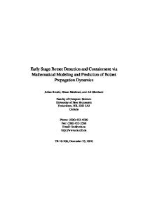
From Eq. 共47兲 it is seen that the zero-order approximation is simply the deterministic ordinary differential equation that would be obtained by setting ⫽0 in Eq. 共43兲, and that the first-order approximation is obtained by linearizing Eq. 共43兲 around the nominal deterministic trajectory obtained from the order zero approximation. We now study the first-order approximation and suppose that Eq. 共48兲 holds for k⫽1 and that z 0 is an interior point of a domain D in R 3 such that the from D is finite. Suppose first exit time t 0 of the process Z (0) t further that the boundary is differentiable at Z t(0) , let ¯n be the 0 exterior normal to the boundary at Z t(0) and denote the first 0 ¯) exit time of the process Z t from D by . Then if (Z˙ (0) t ,n 0
⬎0 we have 关36兴
⫽t 0 ⫹
¯ 共 Z (1) t 0 ,n 兲 ¯ 共 Z˙ (0) t 0 ,n 兲
⫹O 共 兲 ,
共49兲 Z (1) t ⫽
where the remainder term should be interpreted in the sense used in Eq. 共48兲. Hence the first passage time problem for the time varying potential with colored noise can be formulated as the problem of determining in Eq. 共49兲 when x 0 ⬍x limit , where x limit is a barrier for the variable x. In this case ¯n becomes simply ¯n ⫽(0,0,1) T and the condition (0) ¯ )⬎0 in Eq. 共49兲 reduces to x˙ (0) is the (Z˙ t(0) ,n t 0 ⬎0 where x 0 last component in the solution to the first equation in Eq. 共47兲. Since W is a Gaussian process, so is the first-order approximation x (1) , and the first passage time is therefore a Gaussian variable with mean t 0 and a variance 2 E 共 x (1) t 兲 0
V共 兲⫽2
共 x˙ t(0) 兲 2
共50兲
.
0
Further, the 共unique兲 solution to the second equation in Eq. 共47兲 is well known to be 共see, e.g., Ref. 关36兴兲, Z (1) t ⫽
冕
t
0
FIG. 6. The element ⌽ 3,1(t 0 ,t) vs t/T 0 for ⫽0, 2 ⫽0.01, A ⫽0.8, ␥ ⫽1, T 0 ⫽100, start time ⫽0, and the parameters a,b for the equivalent Duffing potential are computed via Eq. 共11兲, for c ⫽4 in the mean field potential 共2兲.
⌽ 共 t,r 兲 g 2 共 Z r(0) 兲 dW r ,
共51兲
where ⌽(t,s) is the transition matrix from time s to t for the flow 共smooth vector field兲 on R 3 defined by (0) (1) Z˙ (1) t ⫽G 31共 Z t ,0 兲 Z t .
冕 冉 冕 t
0
exp ⫺
t
q
冊
G 31共 Z r(0) ,0兲 dr g 2 共 Z (0) q 兲 dW q ,
and Eq. 共50兲 therefore becomes
V共 兲⫽2
⫽2
冕
t0
0
¯n T ⌽ 共 t 0 ,r 兲 g 2 共 Z r(0) 兲 g T2 共 Z r(0) 兲 ⌽ T 共 t 0 ,r 兲¯n dr 兲2 共 x˙ t(0) 0
冕
t0
0
关 ⌽ 3,1共 t 0 ,r 兲兴 2 dr 兲2 共 x˙ t(0) 0
,
共52兲
where ⌽ 3,1(t 0 ,r) is the third row, first column element of ⌽(t 0 ,r). This element is plotted against the normalized time t/T 0 in Fig. 6. Since we have assumed a clearly suprathreshold bias signal, the previous crossing time, i.e., the start time, will be in 关 0,T/2兴 . For all such starting times numerical calculations show that the next deterministic crossing time t 0 is reasonably independent of the starting time 关18兴. Further, as seen in Fig. 6, the function ⌽ 3,1 is close to zero for all t苸 关 0,T/2兴 and therefore the integral in Eq. 共52兲 will also be almost independent of the starting time. Hence all crossing times will be approximately independent and Gaussian distributed with means and variance given by Eqs. 共49兲 and 共52兲, respectively. This has, of course, already been observed in our crude 共Schmidt trigger兲 model of the preceding section in the large A/ limit, when A is well suprathreshold.
In this case the transfer matrix ⌽ is given by
冉冕
⌽ 共 s,t 兲 ⫽exp ⫺
t
s
G 31共 Z r(0) ,0兲 dr
Hence Eq. 共51兲 can be written as
冊
C. Analysis of time-based readout
.
The approximate crossing times distributions calculated in the preceding section are important when evaluating performance measures for ‘‘time-based’’ devices. Since we also want to compare the performance of these devices with the 016120-14
PHYSICAL REVIEW E 67, 016120 共2003兲
SIGNAL DETECTION VIA RESIDENCE-TIME . . .
one obtained under different readout schemes, we have to abandon the SNR in Eq. 共21兲 and move on to a more general performance measure. There exist several possible ways to define such a measure, however, since the expected value of the estimations is correct it seems natural to apply the classic MMSE 关38兴 共minimum-mean-squared-error estimation兲 formalism, and consider the estimator with the lowest variance of the result to be the best. Note, though, that the variance associated with all the estimators will decrease towards zero when the observation time increases. Therefore, a finite observation time T ob is used, and the goodness criterion of the sensors is defined as the variance of the estimation, given this observation time. For residence-time-based devices there will be n(T comp ) switches between the stable states during the observation time. As previously shown, all crossing times will be approximately Gaussian distributed with a mean that depends on the target signal and a variance as in Eq. 共52兲. The dependence between the separation of the mean crossing times and the target signal is linear for small asymmetrizing target signals, i.e., ⫽ c l ,
¯⑀ opt ⫽
兺
i⫽1
n
¯u i ⫺
兺 ¯d i
i⫽1
2n⫹1
cl ,
with a variance V 共 ¯ opt 兲 ⫽
2 c 2l cross
2n⫹1
,
共54兲
which is easily proved by, e.g., the information equality 关37兴. In the previously described approach that measures the mean difference in residence times 具 ⌬T 典 , a displacement cross for the crossing times results in a mean residence-time difference of 4 cross . The estimate of the target signal therefore becomes ¯ res ⫽(c l /4)⌬T, where
冉兺 n
i⫽1
n
共 d i ⫺u i 兲 ⫺
兺 共 u i⫹1 ⫺d i 兲
i⫽1
冊
.
The variance of the residence-time-based estimator will then be
冉 冊
V 共 ¯ res 兲 ⫽V c l
c 2l ⌬T ⫽ V 共 ⌬T 兲 , 4 16
n where V(⌬T)⫽V 关 (1/n) 兺 i⫽1 (2d i ⫺u i ⫺u i⫹1 ) 兴 , which, with the definition Y i ⫽2d i ⫺u i ⫺u i⫹1 , becomes
冉
1 V 共 ⌬T 兲 ⫽V n
n
兺 共Y i兲
i⫽1 n
⫹
兺 兺 i⫽ j j⫽1
冊 冉兺 冊 ⫽
n
1
n2
i⫽1
V共 Y i兲
Cov共 Y i ,Y j 兲 ,
which by straightforward calculations can be shown to be V 共 ⌬T 兲 ⫽
共53兲
where is the change of crossing time and c l a constant. This has already been mentioned in an earlier section, and it can be confirmed by a numerical simulation of the system. The crossing times independence therefore affords the possibility of extracting the optimal achievable limit for any kind of estimator based on crossing times. Let us define ¯u i and ¯d i as ¯u i ⫽u i ⫺u 0 mod(T 0 ) and ¯d i ⫽d i ⫺d 0 mod(T 0 ), i⭓1, where u i and d i are the two 共different兲 crossing times, from one state to the other, and from the second back to the first. Here u 0 and d 0 are the first crossing times in the noise-free system in the absence of the dc target signal. It is readily ¯ i ) and d obtained that cross ⫽ u ⫽⫺ d 关where u ⫽E(u 2 ¯ i )] and cross ⫽ u ⫽ d 关where u ⫽V(u ¯ i ) and 2d ⫽E(d ¯ i )]. The set 兵¯u 1 ,u ¯ 2 , . . . ,u ¯ n⫹1 ,⫺d ¯ 1 ,⫺d ¯ 2 , . . . ,⫺d ¯ n其 ⫽V(d will then consist of 2n⫹1 independent identically distributed Gaussian variables with mean cross and variance 2 cross . In this case it is known from Eq. 共53兲 that the minimum variance estimator of is given by n⫹1
1 ⌬T⫽ n
2 8 cross
n
⫺
2 2 cross
n2
.
Hence, the residence-time-based estimator has the variance V 共 ¯ res 兲 ⫽
冉
2 c 2l 8 cross
16
n
⫺
2 2 cross
n2
冊
⫽
2 c 2l cross
2n
⫺
2 c 2l cross
8n 2
,
which is slightly worse than the optimal time based estimator, Eq. 共54兲, although the performance is comparable 共asymptotically兲 for large n and is much easier to implement in an experiment. In most cases the residence-time-based readout can, therefore, be considered to be the optimal time based readout. D. Comparison of different readouts
In the preceding section we illustrated the advantage of applying the residence-time-based readout scheme, if only sensors involving time measurements were considered. However, it is also instructive to analyze how this readout performs compared to other, more conventional, readout schemes, and to determine the optimal amplitude of the bias signal. Such an investigation is likely to be quite exhaustive, and beyond the scope of the current paper. However, a good starting point is to compare the residence-time-based readout scheme with a ‘‘conventional’’ 共PSD-based兲 readout, when a time-sinusoidal bias signal is applied in each case. This computation will just show the most appropriate amplitude of the sinusoidal bias, with the frequency kept fixed for both devices. This investigation can later easily be expanded to encompass larger signal families. To compare the readouts, n sim , output trajectories x t ,t 苸 关 0,T ob 兴 are calculated for each amplitude of the driving signal. Based on these trajectories n sim , estimates of the target signal are calculated with both the residence-time technique and the conventional 共PSD-based兲 technique, for each amplitude. The variances of these estimates which, according
016120-15
PHYSICAL REVIEW E 67, 016120 共2003兲
BULSARA et al.
to the preceding subsection, could be used as performance measures, are then used to establish the best bias signal amplitude for each method. However, it is also of interest to know how close the sensors are to the optimal performance limit. The optimal performance is given by the MMSE estimator of based on observations of x t over 关 0,T ob 兴 . In case the target signal is a zero mean Gaussian random variable, independent of both the initial condition x 0 and the driving noise, the optimal performance is easy to calculate if the noise is white. Therefore, if we instead of adding the colored noise process t to the state increment dx t in Eq. 共44兲 add a 共scaled兲 Brownian motion increment wg dW t , we obtain the following 共‘‘white noise’’兲 model on SDE form: dx t ⫽ 关 f 共 x t 兲 ⫹⫹h t 兴 dt⫹ wg dW t , where the function f represents the Duffing potential, f (x) ⫽ax⫺bx 3 . The MMSE ˆ of based on x t ,t苸 关 0,T ob 兴 for a system of this type is well known 共Sec. 17.7 of Ref. 关39兴兲 and given by x T ob ⫺x 0 ⫺ ˆ ⫽
冕
T ob
0
关 f 共 x t 兲 ⫹h t 兴 dt
2 wg ⫹T ob 2
,
共55兲
where 2 is the variance of the zero mean Gaussian random variable . When 2 →⬁ the formula 共55兲 becomes identical to that for the maximum likelihood 共ML兲 estimate of 共Sec. 17.7 of Ref. 关39兴兲. Thus, the ML estimator, which is well defined also when is considered as an unknown constant, is a limiting case of the optimal MMSE estimator in Eq. 共55兲 which is obtained when 2 →⬁ 共i.e., when becomes ‘‘completely unknown’’兲. The variance of the ML estimator therefore provides a lower bound on the achievable performance of any estimator of when is an unknown constant. In Fig. 7 the variance of the estimates versus driving signal amplitude is shown for the two different kinds of readout schemes 共residence times, and PSD based兲 and the MLE. As seen, the residence-time-based readout is nearly as good as the PSD-based case, although the sinusoidal bias signal may not be optimal for this sensor 共at least under the parameters considered here兲. A triangular wave, or the wave form 共6兲 should improve the results; as already discussed, these wave forms provide local linearity where the wave form crosses the threshold. Clearly though, both devices perform much worse than the MLE, and it is obvious that both measuring techniques are nonoptimal. From these data it therefore would appear that a MLE-based readout, or a residence-timebased readout with a carefully selected driving signal, would be preferable compared to a PSD-based readout. However, one very surprising result indicates that care should be taken when interpreting the data. The variance of the estimates decreases when the bias amplitude decreases, implying that a weak bias amplitude might be preferable. For the PSD-based readout this is a counterintuitive result since in practical scenarios these sensors are normally driven with a large amplitude bias signal. It is therefore possible that the simple mod-
FIG. 7. The variance of the estimations vs the sinusoidal bias signal amplitude for the residence-time-based 共solid line兲, PSDbased 共dashed line兲, and MLE-based 共bottom dash-dotted line兲 method. Here the parameters a,b, and are as in Fig. 6, ␥ ⫽1, T ob ⫽3000, and the white noise intensity is wg ⫽ 冑2⫻10⫺6 .
els of Sec. II that we use to describe our sensors, may not be good enough. In this context it should be noted that in real sensors involving, e.g., ferromagnetic cores, the noise floor is usually dependent on the driving signal. This is also indicated by the experimental results shown in Fig. 10. In addition, the driving signal, if applied at a sufficiently high frequency, can lead to frequency-dependent hysteresis behavior in the device, behavior that has not been covered by our phenomenological description. Clearly, an investigation of these issues should precede a rigorous investigation 关beyond the relatively simple discussions, in this paper, of the system response to nonsinusoidal wave forms, exemplified by the signal 共6兲兴 into the optimal signal wave form for a particular readout scheme. However, despite these unresolved issues, we can at least conclude that the time series of the output voltage from the fluxgate probe seems to contain more information about the target signal than that which can be extracted via conventional 共PSD-based兲 and residence-timebased readouts. VII. EXPERIMENTS
In order to reconcile some of the ideas of this paper to experimental data some preliminary experiments were performed on a test device, a very simple laboratory realization of a residence-time-based fluxgate magnetometer. A premagnetizing coil with 50 turns and a pick-up coil with 135 turns were wound in a transformerlike configuration on a multidomain ferromagnetic strip-wound ring core characterized by a coercivity of less than 3 A/m. The diameter and the crosssectional area of the ring were 26 mm and 1.9⫻2.8 mm2 ,
016120-16
PHYSICAL REVIEW E 67, 016120 共2003兲
SIGNAL DETECTION VIA RESIDENCE-TIME . . .
respectively. A ring core probe used in this configuration is not expected to possess full directional sensitivity and response to external fields 关2兴. It can, however, serve the purpose of demonstrating the basic principle, without making any claims on living up to the possible operational performance of a fluxgate magnetometer of this type. Note that new, improved probes based on straight rod cores are under fabrication, and the results for these devices will be published later. A function generator producing a triangular wave with variable amplitude A and frequency was connected to the input of the device. A frequency of 100 Hz was used for all measurements. This allows one to use a non-frequency-based description of the crossing dynamics, since frequencydependent hysteresis in the core response is very small and also the bias signal has a minimal effect on the noise floor. The noise floor is assumed to be Gaussian bandlimited, which is a good assumption for the new genre of ‘‘singledomain’’ ferromagnetic probes; non-Gaussian 共i.e., Barkhausen兲 noise may in fact be present in these cores, but it is significantly smaller 共in rms amplitude兲 than the gaussian noise. The 100 Hz driving frequency also ensures that the bias signal does not fall into the low-frequency noise riser. The time evolution of the input current and the output voltage were measured with a 16-bit A/D converter using a sampling rate of 40 kHz. Alternatively, the pick-up coil was connected to a universal counter for measuring the residence times T ⫹ and T ⫺ . The bias field was estimated from the input current by applying Ampere’s law on the ring geometry. The zero target measurements were performed inside a shielded cage consisting of concentrically arranged 共and lidded兲 cylindrical shells made of metal and copper. The measurements with target signal were performed in the presence of the geomagnetic field, which served as the target. They were made after maximizing the effective target strength by simply rotating the device until a maximum difference between 具 T ⫹ 典 and 具 T ⫺ 典 was found. At the location of the experiment this corresponded to a field strength of about 50 T 共the magnitude of the geomagnetic field兲. Figure 8 shows the output voltage from the pick-up coil for four different amplitudes—two subthreshold and two suprathreshold—of the bias signal resulting in nonsaturated and saturated magnetization, respectively. These measurements were performed without target field. The output voltage 共this is our experimental observable兲, which is proportional to the derivative of the magnetic flux in the core, consists of a number of successive spikes corresponding to switches between positive and negative magnetization 共relative to the magnetic state when the bias signal was applied兲. A shift of the spike positions from the extrema towards the zero crossings of the bias signal can be observed as the core material is gradually driven deeper into saturation. For the highest bias amplitude the saturated flux density is rapidly reached and the 共sharp兲 spikes nearly coincide with the zero crossings of the bias signal. The time evolution of the magnetic flux density B in the core material and the magnetization curves were calculated from the experimental data by integrating the output voltage
FIG. 8. Output voltage from the pickup coil for four different amplitudes of the bias field. From left to right A⬇20, 3.3, 2.0, and 1.4 A/m. Bias period T 0 ⫽0.01 s. The dashed curve is a guide for the eyes, and indicates the phase of the bias field.
from the pick-up coil. For each set of data the unknown integration constant was assigned a value in order to make the times series of B centered around zero. The results for two amplitudes of the bias signal (A⫽2 and 20 A/m, corresponding to nearly saturated and saturated cores, respectively兲 are shown as solid curves in Fig. 9. Due to hysteresis effects 共irreversible magnetization兲 changes in the magnetic flux B in the core ‘‘lag behind’’ changes in the magnetizing bias field H. In Fig. 9 this can be observed as a distortion of B from the triangular form of the bias signal and the appearance of hysteresis loops in the magnetization curves. For the saturated case 共right panels兲 B has nearly a rectangular wave form and long tails develop in the magnetization curves. In order to study the ability of the mean field model with the ‘‘soft’’ potential 关Eq. 共2兲兴 to reproduce the experimental details of the ferromagnetic behavior of the core, simulations of B versus time and hysteresis loops were made. In these calculations a dimensionless temperature T⫽1/1.4 (c⫽1.4) was used. The results are shown as dashed curves in Fig. 9. For the saturated case 共right panels兲 the experimental data are quite well described by this model. For the nonsaturated case 共left panels兲, however, only the time evolution of B seems to be fairly well matched. For even lower bias amplitudes the model is unable to reproduce either the time series or the hysteresis loops. Also the equivalent quartic model is unable to reproduce the salient features of the time series and the hysteresis loops at very low 共subthreshold兲 bias amplitudes. This model also fails at extremely high 共very suprathreshold兲 bias amplitudes. Note, however, that despite these discrepancies, both models can reproduce, to a very good approximation, the qualitative behavior in, e.g., 具 ⌬T 典 also for very high suprathreshold bias signals.
016120-17
PHYSICAL REVIEW E 67, 016120 共2003兲
BULSARA et al.
FIG. 9. Upper panels: magnetic flux density vs time of the ferromagnetic ring core for A⫽2 共left panel兲 and 20 A/m 共right panel兲. Lower panels: the same measurement results shown as hysteresis loops. Solid curves are calculated results from experimental data and dashed curves are simulated data using the ‘‘soft’’ potential 共2兲 with c⫽1.4 and A⫽4.0. Note that the B axis has been rescaled for the simulations in order to be able to compare it to the experimental data.
Figure 10 shows the 共Gaussian-like兲 residence-time distributions for three different bias amplitudes A. The data were compensated for offsets 共in the range of about 0.5 to 30 s, with the larger value corresponding to the case of the weakest bias signal兲 which were obtained from zero-field measurements inside the shielded cage. In all cases, the center RTD corresponds to the case of zero target signal. In the presence of a target signal the residence times T ⫹ and T ⫺ are different, and consequently the quantity 具 ⌬T 典 ⫽ 具 T ⫹ 典 ⫺ 具 T ⫺ 典 can be used as a measure of the asymmetryproducing target field. Within our experimental precision a linear relationship between the target signal and 具 ⌬T 典 was found. This is in good agreement with expectations for a pulse-position-based readout technique 关2兴. Such a relationship should be expected 共as already discussed兲 from the RTD-based readout when is small; it has already been theoretically computed in the limiting case of zero bias signal 关9兴. From the slope of a linear fit to the data a response of about 7 ns/ T for our simple test device was found, when it was driven with a 10 kHz bias frequency. Note that this result is not expected to be representative for a well designed device 共currently under construction兲. In Fig. 10 it can readily be seen that the effect of lowering the bias amplitude is twofold. First of all there is an increase in 具 ⌬T 典 for a given target signal strength, and second it leads to a wider spread in the residence times. For example, lowering the bias amplitude from 41 to 20 A/m appears to result in a performance improvement which can be observed as a larger increase in 具 ⌬T 典 as compared to the dispersion of the
FIG. 10. Residence-time distributions for three different amplitudes (⫽41,20, and 4.1 A/m, from top to bottom panels兲 of the triangular bias signal. The data have been normalized to the period T 0 ⫽10 ms. Dashed curves: zero target case. Solid curves: effective target field of about 50 T. The data have been compensated for offsets. The effect of decreasing the bias amplitude is twofold. For a fixed target field the separation 具 ⌬T 典 grows with decreasing bias amplitudes, at which point the fluctuations due to the noise background also manifest themselves in the density function.
RTDs, i.e., the gained response to external target fields seems to be larger than the cost due to a wider spread in the residence times. However, further lowering the bias amplitude down to 4.1 A/m 共where the core material is only weakly saturated兲 a much larger spread in the residence times is observed, and the background noise makes its presence clearly known in the density function for small A. There may be many reasons for this large dispersion at low bias amplitudes. One possible explanation could be that due to the less saturated core material 共and possible memory effects caused by ‘‘noncomplete’’ magnetic domain alignment along the bias field兲 the magnetic hysteresis loop is not well defined. This could, then, lead to varying residence times because different paths around the hysteresis loop may be taken for each cycle. Even in this situation, however, one observes a well-defined 具 ⌬T 典 which, in an experiment, may readily be computed using the arithmetic mean of a large
016120-18
PHYSICAL REVIEW E 67, 016120 共2003兲
SIGNAL DETECTION VIA RESIDENCE-TIME . . .
number N of observed crossing events. We reiterate that, in practical scenarios, a computation of the average residence times via the arithmetic mean is sufficient; it is not necessary to compute a density function and then compute the means via integration. Hence, the accuracy of the measurement of 具 ⌬T 典 depends on the magnitude of N. Of course, the magnitude of N is constrained by the observation time as already discussed in Sec. V. Despite the crudeness of the setup, the experimental findings do qualitatively agree with the results of the simulations shown in Fig. 4. This, in turn, has led to the 共currently ongoing兲 construction of a fluxgate magnetometer utilizing the residence-time-based readout scheme. One important task when optimizing the bias signal for a real device would then be to find the optimum balance between the gain in responsivity and the increase in the noise level of the residence times. VIII. CONCLUSIONS
In this work we have presented an alternative to quantifying the output of a nonlinear dynamic system via the power spectral density. The residence-time-based technique is relatively simple to implement in practical scenarios; all that is required is for the detection/processing electronics to keep track of threshold crossing events and maintain a running average, the arithmetic mean, of the residence times in each stable state. Then the quantity 具 ⌬T 典 provides a measure of the unknown target signal that created the asymmetry and, therefore, a nonzero 具 ⌬T 典 . While the target signal in this work is taken to be dc, it is clear that a modification of the residence-time-based readout scheme could be effected for more complex signals. It is also clear that the choice of the bias signal wave form is important to the issue of overall sensitivity defined, roughly, as the ability to discriminate the means of the residence-time densities in the presence of a small asymmetrizing target signal. The bias signal amplitude does not need to be extremely large. In fact, our results, and those of our earlier publication 关9兴, indicate that the best response to the target signal is obtained for zero bias signal, in theory, at least. In this scenario the level crossing events are solely controlled by the background noise. In practice, however, unless the noise level is high enough to induce an acceptable 共spontaneous兲 crossing rate, one must impose the bias signal to control the crossings. In this case the noise leads to a spread in the crossing rate about its deterministic value, when the bias signal is suprathreshold. Clearly, in such a situation, it would be preferable to adjust the system parameters 关e.g., the constant c in the potential energy function 共2兲兴 so that the energy barrier is lowered when weak target signals are to be detected in a noise floor. In the absence of such a control, however, adjusting the bias amplitude A, or the triangular signal amplitude 2 when we use the bias wave form 共6兲, effectively raises or lowers the energy barrier. With a large background noise floor, the density functions tend to merge, leading to inaccuracies in the computed 具 ⌬T 典 unless a large number N of observations can be made. Increasing A enables one to better resolve the density functions, even as it leads to a greater power requirement.
Hence, one must also consider the tradeoff between sensitivity and power when designing a sensor aimed at a particular class of target signals. Noise effects become more important as the bias signal amplitude approaches the threshold; the RTD is no longer Gaussian, it develops tails and its mean and mode separate. A theoretical computation of 具 ⌬T 典 has been carried out in the regime of large 共suprathreshold兲 bias signal and small noise; in this 共Gaussian兲 limit, the dynamical system is well approximated by a nondynamical dual-threshold representation. For small target signals one easily obtains 具 ⌬T 典 ⬀. The separation 具 ⌬T 典 is, further, very weakly dependent on the noise in the large A/ limit 共the Gaussian limit that has featured so prominently in our discussion兲. In this limit, the noise statistics, also, do not have a significant effect on 具 ⌬T 典 . For subthreshold bias signals, the theory of this paper breaks down. In practical operation, however, one can still compute 具 ⌬T 典 by simple averaging as done for the suprathreshold bias case; in this case, however, the mean value separation is noise-dependent and one may optimize it using the SR scenario 关6兴. The RTD for subthreshold bias signals can be multimodal 共depending on the noise variance, signal amplitude, and potential barrier height兲, however, in the optimal case it collapses into a single near-Gaussian peak at T 0 /2. This case underpins the interpretation of SR as a bona fide resonance 关7兴. Note that for the subthreshold bias signal case, one may compute 关13兴 the residence times in the A/ Ⰶ1 limit 共the often-discussed SR regime兲. The case of strong 共but still subthreshold兲 bias signals and weak noise, i.e., A/ Ⰷ1 has recently been analyzed in some detail 关40兴. In this regime, one obtains a near-exponential dependence of 具 ⌬T 典 on the asymmetrizing signal ⑀ , indicating that optimal sensitivity in this technique might be achievable for bias signal amplitudes hovering around the threshold of the energy barrier. Assuming prior knowledge of the sensor characteristics, it is reasonable to expect that one could determine the energy barrier height in practical applications, thereby affording a convenient route to setting the known bias amplitude. The bias frequency does not figure prominently into the crossing statistics when we work in the nondynamical limit; however, in the general case, the frequency must be carefully selected. In some ferromagnetic cores, employed, for instance, in the simple magnetometer used in our experiments, the 共non-Gaussian兲 Barkhausen noise floor depends on the bias frequency, through its effect on the slip dynamics of the domain walls; usually there exists a 共material-dependent兲 optimal frequency at which these effects are negligible 关30兴. Also, for the case of a soft ferromagnetic core the width of the hysteresis loop, which determines the energy dissipated per cycle, can depend on the frequency and amplitude of the bias signal. Keeping the bias signal amplitude and frequency as low as possible can lead to significantly reduced on-board power; in a real device, this can be an important consideration. However, clearly, the tradeoff between on-board power and the observation time T ob —which determines the accuracy of the experimental estimate of the quantity 具 ⌬T 典 —eventually dictates how the sensor is operated.
016120-19
PHYSICAL REVIEW E 67, 016120 共2003兲
BULSARA et al.
planar device, developed in PCB technology, and boasts dimensions small enough to fit comfortably 共minus the readout electronics兲 into a small cigarette pack. The instrument employs a triangular bias wave form and a very simple digital counter to keep track of the crossing events 关41兴. The laboratory device 共excluding the readout electronics兲 costs about $1, and has an amorphous metal 共or metallic glass alloy, Metglass兲 core. Current experiments, ongoing at the University of Catnaia, Italy, are aimed at enhancing its sensitivity/ resolution by incorporating this device into a coupled array, with the ultimate goal of constructing a network of fluxgates using MeMs technology. It is worth pointing out that the idea of threshold crossing events leading to a quantification of external signals is deeply rooted in the computational neuroscience repertoire wherein one analyzes the response of a single neuron, or even a small network, to a stimulus by examining the statistics of the point process generated by successive threshold crossings or ‘‘firings.’’ This point has already been touched on in Sec. I, but it is important enough to reiterate in this section: our proposed mode of operation actually leads to an implementation of these sensors as ‘‘neural’’-like devices. Subsequent work must focus 共among other issues兲 on the determination of the optimal bias signal wave form in terms of specific sensor and operational parameters. Clearly, there could be other wave forms besides the sinusoidal bias and wave form 共6兲 that might be optimal under different conditions. Continued investigations into the 共non-Gaussian兲 material-dependent noise floor are also important, although, as exploited in this work, this noise may effectively be characterized as Gaussian bandlimited noise subject to the appropriate fabrication, materials, and geometry constraints.
The proposed technique is part of the genre of systems operated based on their level crossing dynamics. It should be readily applicable to a large class of dynamic sensors that are operated as detectors of very small target signals, particularly when the detection scheme and the sensor dynamics lend themselves to operation under a known bias signal whose wave form must be carefully selected for optimal sensitivity. In this context we reiterate that the time-sinusoidal bias signal is not necessarily the wave form that yields the best output sensitivity 共or resolution兲. The rigorous analysis of Sec. VI indicates, in fact, that with the time-sinusoidal bias waveform one might expect the RTD-based approach to yield sensitivity comparable to conventional 共PSD-based兲 techniques. However, we hasten to point out that, while the analysis of Sec. VI was carried out in the context of a sinusoidal bias wave form, one would usually use a triangular wave form, or wave form 共6兲 in practice. Both these wave forms outperform the sinusoidal wave form, and they also enable the RTDbased approach to outperform conventional processing. In addition, one must take into account the inherent simplicity of the RTD approach, particularly with regard to the readout electronics and processing. Typically, a simple counting circuit is required, in contrast to the feedback electronics that are usually a part of readout schemes; more complicated electronics usually add more noise to the already present noise floor. By contrast, in our simple experiments on the prototype nonlinear dynamic sensor 共the fluxgate magnetometer兲 described in the preceding section, one can implement the RTD readout with just one excitation coil and one detection coil without the need for implementing a differential structure 共usually done to cancel out steady ambient magnetic fields兲. Most importantly, the RTD approach can be implemented with low-amplitude and low-frequency bias signals which result in significantly reduced on-board power requirements. In addition to the experiments described in the preceding section, another laboratory prototype fluxgate magnetometer, using the RTD technique, has already been constructed and operated via the procedure described in this work. It is a
We gratefully acknowledge funding from the Office of Naval Research Code 331. M.K., B.L., and J.R. acknowledge funding under the Sweden Armed Forces, Contract No. E6706.
关1兴 See, e.g., W. Geyger, Nonlinear Magnetic Control Devices 共McGraw-Hill, New York, 1964兲; P. Ripka, Sens. Actuators A 33, 129 共1992兲. 关2兴 W. Bornhofft and G. Trenkler, in Sensors, A Comprehensive Survey, edited by W. Gopel, J. Hesse, and J. Zemel 共VCH, New York, 1989兲, Vol. 5. 关3兴 See, e.g., A. Barone and G. Paterno, Physics and Applications of the Josephson Effect 共Wiley, New York, 1982兲; J. Clarke, in The New Superconducting Electronics, edited by H. Weinstock and R. Ralston 共Kluwer Amsterdam, 1993兲. 关4兴 See, e.g., I. Bunget and M. Prohescu, Physics of Solid Dielectrics 共Elsevier, New York, 1984兲; D. Damjanovic, P. Muralt, and N. Setter, IEEE Sensors Journal 1, 191 共2001兲. 关5兴 See, e.g., J. Fraden, Handbook of Modern Sensors 共AIP Press, New York, 1997兲, and references therein; W. Bornhofft and G. Trenkler, in Sensors, A Comprehensive Survey, edited by W.
Gopel, J. Hesse, and J. Zemel 共VCH, New York, 1992兲 Vols. 1 and 2. For reviews see, A. R. Bulsara and L. Gammaitoni, Phys. Today 49 共3兲, 39 共1996兲; L. Gammaitoni, P. Hanggi, P. Jung, and F. Marchesoni, Rev. Mod. Phys. 70, 223 共1998兲. L. Gammaitoni, F. Marchesoni, and S. Santucci, Phys. Rev. Lett. 74, 1052 共1995兲. R. Bartussek, P. Hanggi, and P. Jung, Phys. Rev. E 49, 3930 共1994兲; A.R. Bulsara, M.E. Inchiosa, and L. Gammaitoni, Phys. Rev. Lett. 77, 2162 共1996兲; M.E. Inchiosa, A.R. Bulsara, and L. Gammaitoni, Phys. Rev. E 55, 4049 共1997兲. L. Gammaitoni and A. Bulsara, Phys. Rev. Lett. 88, 230601 共2002兲. M. Inchiosa and A. Bulsara, Phys. Rev. E 53, R2021 共1996兲; C. Heneghan, C.C. Chow, J.J. Collins, T.T. Imhoff, S.B. Lowen, and M.C. Teich, ibid. 54, R2228 共1996兲; F. Chapeau-Blondeau,
ACKNOWLEDGMENTS
关6兴
关7兴 关8兴
关9兴 关10兴
016120-20
PHYSICAL REVIEW E 67, 016120 共2003兲
SIGNAL DETECTION VIA RESIDENCE-TIME . . .
关11兴 关12兴 关13兴
关14兴
关15兴
关16兴 关17兴 关18兴
关19兴 关20兴
关21兴 关22兴 关23兴
ibid. 55, 2016 共1997兲; V. Galdi, V. Pierra, and I. Pinto, ibid. 57, 6470 共1998兲; J. Robinson, D. Asraf, A. Bulsara, and M. Inchiosa, Phys. Rev. Lett. 81, 2850 共1998兲; M. Inchiosa, J. Robinson, and A. Bulsara, ibid. 85, 3369 共2000兲; S. Kay, IEEE Signal Process. Lett. 7, 8 共2000兲; I. Goychuk and P. Ha¨nggi, Phys. Rev. E 61, 4272 共2000兲; J. Robinson, J. Rung, A. Bulsara, and M. Inchiosa, ibid. 63, 011107 共2001兲. M. Inchiosa and A. Bulsara, Phys. Rev. E 58, 115 共1998兲. L. Gammaitoni, F. Marchesoni, E. Menichella-Saetta, and S. Santucci, Phys. Rev. Lett. 62, 349 共1989兲. T. Zhou, F. Moss, and P. Jung, Phys. Rev. A 42, 3161 共1990兲; P. Jung, Phys. Rep. 234, 175 共1993兲; M. Choi, R. Fox, and P. Jung, Phys. Rev. E 57, 6335 共1998兲. See, e.g., H. Tuckwell, Introduction to Theoretical Neurobiology 共Cambridge Univ. Press, Cambridge 1988兲. A. Longtin, A. Bulsara, and F. Moss, Phys. Rev. Lett. 67, 656 共1991兲; A. Longtin, A. Bulsara, D. Pierson, and F. Moss, Biol. Cybern. 70, 569 共1994兲; C. Koch, Biophysics of Computation 共Oxford Univ. Press, New York, 1999兲; A. Longtin, in Stochastic Dynamics and Pattern Formation in Biological Systems, edited by S. Kim, K. J. Lee, and W. Sung 共AIP Press, New York, 2000兲. See, e.g., D. Cox, Point Processes 共CRC Press, New York, 1980兲; D. Cox and H. Miller, Stochastic Processes 共Chapman and Hall, London, 1996兲. See, e.g., G. Papoulis, Probability, Random Variables, and Stochstic Processes 共McGraw-Hill, New York, 1991兲. J. Millman, Microelectronics 共McGraw-Hill, New York, 1983兲. M. Karlsson, J. Robinson, A. Bulsara, and L. Gammaitoni, in Proceedings of the Marine Electromagnetics Meeting (MARELEC), Stockholm, 2001 共Spearhead Group, U.K., 2001兲, available on CDRom only. M. Rao and R. Pandit, Phys. Rev. B 43, 3373 共1991兲. In these units the Curie temperature T c ⫽zJ/k B is set equal to unity, where z is the number of nearest neighbors, J is the strength of the exchange interaction, and k B is the Boltzmann’s constant. For a very good overview, see, e.g., G. Bertotti, Hysteresis in Magnetism 共Academic Press, San Diego, 1998兲. See, e.g., H. E. Stanley, Introduction to Phase Transitions and Critical Phenomena 共Oxford Univ. Press, Oxford, 1971兲. T. Tome and M. de Oliveira, Phys. Rev. A 41, 4251 共1990兲; M. Rao, H. Krishnamurthy, and R. Pandit, Phys. Rev. B 42, 856 共1990兲; M. Zimmer, Phys. Rev. E 47, 3950 共1993兲; B. Chakra-
关24兴 关25兴
关26兴 关27兴
关28兴 关29兴 关30兴
关31兴 关32兴
关33兴
关34兴
关35兴 关36兴 关37兴 关38兴 关39兴 关40兴 关41兴
016120-21
varty and M. Acharya, Rev. Mod. Phys. 71, 847 共1999兲; H. Fujisaka, H. Tutu, and P. Rikvold, Phys. Rev. E 63, 036109 共2001兲. S. Sides, P. Rikvold, and M. Novotny, Phys. Rev. Lett. 81, 834 共1998兲; Phys. Rev. E 59, 2710 共1999兲. Z. Neda, Phys. Rev. E 51, 5315 共1995兲; S. Sides, P. Rikvold, and M. Novotny, ibid. 57, 6512 共1998兲; S. Sides, Ph.D. dissertation, Florida State University, 1998 共unpublished兲. W.F. Brown, Phys. Rev. 130, 1677 共1963兲. T.L. Gilbert, Phys. Rev. 100, 1243 共1955兲; L. Landau and E. Lifshitz, Electrodyanmics of Continuous Media 共Pergamon, New York, 1960兲. A. Perez-Madrid and J.M. Rubi, Phys. Rev. E 51, 4159 共1995兲. B. McNamara and K. Wiesenfeld, Phys. Rev. 39, 4954 共1989兲. J. Deak, A. Miklich, J. Slonczewski, and R. Koch, Appl. Phys. Lett. 69, 1157 共1996兲; R. Koch and J. Rozen, ibid. 78, 1897 共2001兲. See, e.g., C. Gardiner, Handbook of Stochastic Methods 共Springer-Verlag, Berlin, 1985兲. L. Gammaitoni, F. Marchesoni, E. Menichella-Saetta, and S. Santucci, Phys. Rev. Lett. 62, 349 共1989兲; A. Longtin, A. Bulsara, and F. Moss, ibid. 67, 656 共1991兲; Mod. Phys. Lett. B 6, 1299 共1992兲; A. Longtin, A. Bulsara, D. Person, and F. Moss, Biol. Cybern. 70, 569 共1994兲. P. Ha¨nggi and P. Jung, Adv. Chem. Phys. 89, 239 共1995兲; P. Ha¨nggi, M. Inchiosa, D. Fogliatti, and A. Bulsara, Phys. Rev. E 62, 6155 共2000兲. F. Apostolico, L. Gammaitoni, F. Marchesoni, and S. Santucci, Phys. Rev. E 55, 36 共1997兲; F. Marchesoni, F. Apostolico, L. Gammaitoni, and S. Santucci, ibid. 58, 7079 共1998兲. See, e.g., N. Bleistein and R. Handelsman, Asymptotic Expansions of Integrals 共Dover, New York, 1986兲. M. I. Freidlin and A. D. Wentzell, Random Perturbations of Dynamical Systems 共Springer-Verlag, Berlin, 1998兲. T. Cover and J. Tomas, Elements of Information Theory 共Wiley, New York, 1991兲. H. V. Poor, An Introduction to Signal Detection and Estimation 共Springer-Verlag, Berlin, 1988兲. R. S. Liptser and A. N. Shiryayev, Statistics of Random Processes II 共Springer-Verlag, New York, 1978兲. A. Nikitin, N. Stocks, and A. Bulsara, Phys. Rev. E 共to be published兲. B. Ando, S. Baglio, A. Bulsara, and L. Gammaitoni, IEEE Trans. Magn. 共to be published兲.