SEPARATION OF SNR VIA DIMENSION EXPANSION IN A MODEL OF THE CENTRAL AUDITORY SYSTEM Woojay Jeon and Biing-Hwang Juang Georgia Institute of Technology School of Electrical and Computer Engineering Atlanta, GA 30332 ABSTRACT In this study, we provide a theoretical approach for analyzing signal and noise separation and the noise-robustness of class-dependent activation areas in a model of the primary auditory cortex in the central auditory system. Specifically, we interpret the auditory model as a system of localized matched filters that act as a place-coding mechanism for mapping signal and noise spectra into separate regions in the three-dimensional cortical space. This framework allows us to analyze the noise robustness of signal-respondent neurons by computing their signal-to-noise ratio(SNR)’s without having to explicitly consider the complex mathematical expressions for the auditory model. The framework is also fundamentally consistent with the notion of category-dependence proposed in our previous work. Our theoretical developments of the place-coding effect and the separation of SNR will be also demonstrated experimentally. 1. INTRODUCTION
2. GENERAL FRAMEWORK 2.1. Best-match response areas and place-coding Let p(y) denote the power spectrum of an uncorrupted signal defined on the frequency domain y. The cortical response r (y; λ) represents the amount of activation of a neuron that takes on a specific neural response area[2]. Mathematically, the response is defined as the inner product between p(y) and the response area function w(y; λ) parameterized by λ, which consists of best frequency(BF) x, scale s, and symmetry φ. Since w (y; λ) is a local response area, we assume that it is meaningful over some region R(λ) and is zero elsewhere. We also assume that w(y; λ) satisfies the constraint: � w2 (y; λ)dy = k (1) R(λ)
In previous studies, we experimentally established the relevance[1] of a variant of a model of the primary auditory cortex(A1) in the central auditory system[2], and were able to obtain improved recognition results under noisy conditions by introducing a phoneme category-dependent feature selection method[3] based on conjecture on the category-dependent place-coding of cognitive information. In this study, we will propose an analytical approach for studying the effects of noise on the cortical response by recognizing that the cortical transformation acts as a system of localized matched filters that map signal and noise spectra to different locations in the cortical space. The localized nature of each matched filter allows the transformation to place-code spectral components in a dimensionexpanded space where they can each be isolated and accessed in a more explicit form. This is fundamentally different from the traditional cepstrum, which is a transformation that simply results in a sinusoidal decomposition of the log power spectrum. The matched filter perspective allows us to analyze the noise robustness of cortical neurons by approximating the response areas as functions of the signal spectral envelopes, without having to directly manipulate the complex mathematical equations that model excitation and inhibition. Through this analysis, we can compute the SNR of signal-respondent cortical neurons under simplified conditions to show that the separation of spectral components allows signal-respondent cortical neurons to be robust toward noise when signal and noise are combined. These effects will also be demonstrated experimentally using samples of speech phonemes. Furthermore, the dependence of noise robust, signal-respondent cortical locations on the structure of the frequency-domain power spectrum implies that these regions will be signal category-dependent,
142440469X/06/$20.00 ©2006 IEEE
which is, at a conceptual level, consistent with our previous work on category-dependent feature selection[3].
The cortical response is: r (λ) =
� R(λ)
p (y) w (y; λ) dy
(2)
Assume that we are interested in the function w(y; λ) that will provide the maximum squared (or absolute) response. By the CauchySchwarz Inequality, we have: � r2 (λ) ≤ k p2 (y) dy (3) R(λ)
where the maximum will occur when: w (y; λ) = c · p (y) (4) in R(λ) where c is a constant designed to satisfy (1). Hence, it is generally the response area that most closely matches the shape of the spectrum (as in Fig. 3(a), (b), (d)), or its mirror (when c < 0 as in Fig. 3(c)) in a given local region that will result in the highest response. This was also observed in the original development of the model[2]. We can see that the cortical transformation acts like a system of localized matched filters[4], where each response area is designed to mimic the shape of a local spectral component. While narrow response areas that model individual peaks give high response in harmonics of the spectrum as in Fig. 3(a), it is often response areas that match the broadband envelope of the spectrum that yield the strongest output, as in Fig. 3(b) and (c). For instance, assume that the power spectrum takes on the following form: � δ (y − k∆) v (y) (5) p (y) = k∆∈R
where the summation is performed over the integer k and R is the entire frequency range of interest. In a speech signal, ∆ models the
I 1233
ICASSP 2006
pitch, while v(y) is the spectral envelope that can model broadband energy distributions such as formants. We have: � � �2 v (k∆) w (k∆; λ) (6) r2 (λ) = k∆∈R(λ)
If ∆ is small compared to R(λ), (1) also implies: � � K 1 w2 (y; λ)dy = w2 (k∆; λ) ≈ ∆ R(λ) ∆
(7)
k∆∈R(λ)
By the summation form of the Cauchy-Schwarz Inequality, the maximum response will occur when w (k∆) is a constant multiple of v (k∆) in R(λ). One response area function that satisfies this is: � c · v (y) y ∈ R (λ) w (y; λ) = (8) 0 y∈ / R (λ) and we now have a response area that traces the spectral envelope. The localized matched filtering also implies a place-coding mechanism in the cortical transformation. Consider the addition of some wide sense stationary noise in the time-domain that results in a corrupted spectrum written as follows: (9) p (y)� = p (y) + d (y) Continuing our line of thought, when the input is noise alone, the cortical transformation over the region R(λ) will be maximum for the neuron, if any, that has a response area of this form: � c · d (y) y ∈ R (θ) = R (λ) (10) w (y; θ) = 0 y∈ / R (θ) = R (λ) Now, assume the signal power spectrum takes on the impulse train form in (5). For this signal, the best matching response area function is that given in (8). Hence, the signal and noise will each have its own distinct maximally-respondent neuron. Neurons surrounding the maximally-respondent ones will also have high responses since their response areas are similar. In summary, as long as the signal spectrum and noise spectrum are different, the signal and noise tend to have different areas of activation in the cortical space. For example, it can can be clearly observed in Fig. 2 ∼ 5 that the signalrespondent components and the noise-respondent components are mapped to distinct regions in the cortical space. Note that the localized nature of the response area plays an important role in place-coding because it allows the response areas to replicate parts of the spectrum in a divide-and-conquer-like manner as in Fig. 3 and 5 without having to match the spectrum in its entirety. Also note that the transformation in (2) is equivalent to the Fourier transform if the response areas are sinusoids spanning R. If p(y) is a log spectrum, this results in the cepstrum. However, from the matched filter perspective, the cepstrum is fundamentally different in that it is merely a sinusoidal decomposition of the power spectrum because the transformation functions are simple sinusoids spanning the entire frequency range, not localized response areas designed to collectively match the actual structure of the spectrum. 2.2. Noise-robustness When signal and noise are combined, both the signal-respondent neuron in (8) and the noise-respondent neuron in (10) carry both signal and noise components due to the additive nature of the cortical transformation. We can show, however, that the signal-respondent neuron is robust toward noise. By (2) and (9), the response to the combination of signal and noise is : � � r (λ)� = p (y) w (y; λ) dy + d (y) w (y; λ) dy (11) R(λ)
R(λ)
We define the SNR of the response as the ratio between the signalrespondent neuron’s activation by the clean signal, and the distortion
inflicted on the same neuron by the addition of noise. Since in the actual model the cortical response can be negative due to inhibitory regions in w(y), we take the absolute value to represent response power. The motivation behind this equation is that p(y) is already a measure of signal power, and viewing the cortical response as a weighted sum of the power spectrum, we want to preserve the units. �� � � � � R(λ) p (y) w (y; λ) dy � |r (λ)| � � � Sr,λ = �� = (12) � �� r (λ)� − r (λ)� � R(λ) d (y) w (y; λ) dy � We can also define the SNR of the power spectrum in R(λ) before cortical transformation. � p (y) R(λ) Sp,λ = � (13) |d (y)| R(λ) In the auditory spectrum [5] used in our physiological model, d(y) can be negative, which is why we include an absolute value sign. Now, assume that the noise is stationary white noise with variance β over R, and p(y) is the Fourier power spectrum. This results in d(y) = β. Assuming the harmonic model in (5), the SNR of the noise-respondent neuron with response area defined in (10) is: � v (k∆) cβ � k∆∈R(λ) 1 � v (k∆) (14) Sr,θ = = βVλ c R(λ) β 2 dy k∆∈R(λ)
where Vλ denotes the volume (length in 1-d case) of the region R(λ). It is also easy to see that this is the SNR of the spectrum in (13): (15) Sr,θ = Sp,λ The SNR of the signal-respondent neuron with response area (8) is:
2 � � 2 1 v (k∆) v (k∆) c n k∆∈R(λ) k∆∈R(λ) � � Sr,λ = ≥ (16) cβ R(λ) v (y) dy β R(λ) v (y) dy where n denotes the number of harmonic impulses in R (λ) and we have applied the summation form of the Cauchy-Schwarz Inequality where equality holds when all v(k∆) are equal. If the pitch ∆ is small compared to R (λ), � � v (y) dy ≈ ∆ v (k∆) R(λ)
(17)
k∆∈R(λ)
In addition, we know that n∆ ≈ Vλ . Hence, � 1 v (k∆) = Sr,θ = Sp,λ Sr,λ ≥ βVλ
(18)
k∆∈R(λ)
Hence, we can see that the signal-respondent neuron has an SNR that is greater than both the SNR of the noise-respondent neuron and the average SNR of the input signal in R(λ). The same result can also be achieved if we simply assume that the peaks contain enough energy such that the envelope is a close approximation of the spectrum, i.e., p(y) ≈ v(y). The relation can break down if the response area does not encompass a broad range of harmonic peaks as assumed in (17), or, stated from a different perspective, if the envelope v(y) is too different from the spectrum p(y) in R (λ). To measure the collective effect of cortical transformations, we can define the overall SNR of a set A = {λi } of cortical neurons, and the overall SNR of the power spectrum as: � � |r (λi )| p (y) λi ∈A R � , S Sr (A) = � � (19) = p � �r (λi )� − r (λi )� |d (y)|
I 1234
λi ∈A
R
α
2
1.0
Scale (cyc/oct)
� 2 2 Sr,λ Sr,Λ 2s1 s2 s21 + VΛ s2 γ
b
Fig. 1. Ratio of squared SNR’s as a function of b Note that Sp is simply Sp,λ with R(λ) = R, and in the case of d(y) = β denotes the overall SNR of the time-domain signal. Now, even if all neurons in A satisfied (18), this does not necessarily imply Sr (A) ≥ Sp . However, since any lower bound on Sr,λ for all λ ∈ A is a lower bound for Sr (A), there is a good chance of Sr (A) ≥ Sp as long as A is carefully selected. This turns out to be demonstrable in practice, as we will show in Section 3.
where b > 0 and Λ is some {x, s, φ}. By subtracting a constant from the spectrum, we divide it into a positive region and a negative region, which are effectively matched with the excitatory and inhibitory regions of the response area. Intuitively, this makes sense because the inhibitory regions and excitatory regions tend to cancel each other, and in order to minimize this cancelation the largest spectral components should match the excitatory regions and the smallest spectral components should match the inhibitory regions as in Fig. 3(a), (b) and, (d), or vice versa as in 3(c). To see how this affects our analysis of the SNR, we first assign the following variables for notational simplicity. � � s1 = R(Λ) v (y) dy, s2 = R(Λ) v 2 (y) dy (21) Again, by invoking the approximation in (17), we have: � � � � 1 �� s2 �� 1 �� s2 − bs1 �� , S = Sr,Λ = r,λ ∆β � s1 − bVΛ � ∆β � s1 �
(a)
2.0 1.0
(d)
0.5
(c)
(b) 0.5 1.0 2.0 4.0 Frequency (kHz) Fig. 2. a(x, s) of a steady segment of an “aa” phone. Dark is high.
0.25
80
20
40
10
0
2.3. Modeling inhibition in the cortical response The response areas in the actual cortical response are constrained to have excitatory lobes flanked by inhibitory lobes of varying scale and symmetry[1]. Therefore, (8) in the general framework can be modified to more reasonably approximate the signal-respondent response areas by adding a bias term as follows: � c · {v (y) − b} y ∈ R (Λ) (20) w (y; Λ) = 0 y∈ / R (Λ)
4.0
0 0.25 1.0 4.0 kHz (a) x=330, s=3.5, φ=5.6
20 10 0
0.25 1.0 4.0 kHz (b) x=523, s=0.26, φ=17 20 10 0 −10
0.25 1.0 4.0 kHz 0.25 1.0 4.0 kHz (c) x=1209, s=0.43, φ=90 (d) x=1865, s=0.72, φ=90 Fig. 3. The auditory spectrum of a steady “aa” phone, and response areas corresponding to components labeled in Fig. 2. Units for x, s, and φ are Hz, cyc/oct, and degrees, respectively. The x-axis is tonotopic frequency, and the y-axis has arbitrary units indicating the magnitude of the response areas and the auditory spectrum. assume that the b for the cortical response areas, as those shown in Fig. 3, will roughly lie in the vicinity of γ due to their symmetry, particularly when φ = ±π/2. However, since distortion in the cortical response greatly differs from a constant, the change in SNR will not follow the illustrated curve exactly. 3. EXPERIMENTS
(22)
We can compare the two SNR’s by taking the squared ratio and writing it as a function of b as follows: � 2 � 2 2 Sr,Λ s1 (bs1 − s2 ) ρ = = α + (23) 2 Sr,λ s2 (bVΛ − s1 ) b−γ where
� s1 s21 − VΛ s2 s21 s1 α= , ρ= (24) , γ= s2 VΛ VΛ s2 VΛ2 By the integral form of the Cauchy-Schwarz relation, and ignoring the equality case which would � require the spectral envelope to be constant, we have s2 > s21 VΛ . Hence, we know that 0 < α < 1 and ρ < 0, and also γ > 0. It is easy to visualize (23) as Fig. 1 and recognize that Sr,Λ > Sr,λ as long as: 2s1 s2 (25) 0
As stated in [2], it is yet unclear how the response areas in the cortical response should be normalized. If w (y; x, s, φ)� denotes the existing response areas used in the current auditory model[1], it is easy to show that (1) will be satisfied if: 1 (26) w (y; x, s, φ) = √ s w (y; x, s, φ)� α That is, the currently-existing response areas are essentially similar to the normalized ones, only, there exists a bias that causes them to favor low-bandwidth (high s) response areas more. However, for a given scale s, which roughly translates to a fixed volume Vλ , the cortical response will behave exactly the same as when using the normalized response areas. Hence, we believe the matched filter framework essentially remains valid for the current model. The response a(x, s) is provided by the neuron with φ that gives the highest response for a neighborhood of x roughly defined by s: a (x, s) = max |r (x, s, φ)| (27) φ
Fig. 2 shows a(x, s) for a steady segment of the “aa” phone. The areas with highest response constitute the signal-respondent cortical neurons. As labeled in the diagram, we can see how the harmonic (a), broadband energy (b), trough (c) (for which c < 0 in (20)), and formant in (d) map to separate regions. Although phase information is lost in the diagram, one can see in Fig. 3 that the signal-respondent
I 1235
SNR (dB)
Scale (cyc/oct)
4.0 2.0 1.0 0.5
(a)
0.5 1.0 2.0 4.0 Frequency (kHz) Fig. 4. a(x, s) of the averaged distortion of the “aa” phone in Fig. 2 for input SNR 5 dB.
5
0.25 0.5 1.0 2.0 4.0 Frequency (kHz) Fig. 6. Sr (A(x)) (thick line), Sr (A) (solid horizontal line), and Sp (dotted horizontal line). Sr (A(x)) does not exist for x > 3 kHz because no signal-respondent response with best frequency in that range exists.
Ratio
5
0 −5
10 0
(b)
0.25
5
15
0
0.25 1.0 4.0 kHz 0.25 1.0 4.0 kHz (a) x=2154, s=0.40, φ=-90 (b) x=4699, s=0.33, φ=-34 Fig. 5. Response areas of key components in Fig. 4. Units are the same as in Fig. 3. Most of the noise is mapped to cortical regions that are separate from the signal-respondent regions in Fig. 2. clumps of neurons also have different phases, which means that they form separate clusters in the 3-d cortical space. Fig. 4 shows a(x, s) of the distortion d(y) for the same “aa” phone segment. In order to remove statistical variation, we computed the mean of the combined spectrum in (9) over many instances of additive white Gaussian noise in the time-domain, and then subtracted the signal spectrum p(y) to obtain d(y). As shown in Fig. 5, d(y) is not constant and has some dependency on the signal spectrum due to the noise suppression action of the auditory spectrum[6]. We can clearly see how the noise components map to areas different from the signal-respondent areas. In particular, 4(a) does not overlap with 2(c) and 2(d) much because they have different values of φ. Hence, the signal-respondent areas are able to stay intact when signal and noise are combined. The SNR of signal-respondent neurons is also demonstrated for the same signal. We applied a threshold on r(λ) to obtain a set A of signalrespondent neurons that include the major activation areas in Fig. 2. In Fig. 6, we have indicated the overall SNR’s Sr (A) and Sp defined in (19). To provide some sense of how the noise robustness of signal-respondent areas changes for varying best frequencies, we also plotted a localized SNR Sr (A(x)) where A (x) is the set of signal-respondent neurons in A with BF x. Finally, in Fig. 7 we computed SNR’s for 44 phoneme classes in the TIMIT database for various input SNR under stationary Gaussian white noise, using all samples from training data excluding “sa” sentences. For each phoneme class, A in (19) was constructed by finding the neurons with the top 4% absolute response, averaged over all samples of the given class. U is the entire set of cortical neurons. The mean of the ratios Sr (A)/Sp and Sr (A)/Sr (U ), taken over all phoneme segments, are plotted and compared to 1 to illustrate how the signal-respondent neurons generally have higher SNR. 4. CONCLUSION AND FUTURE WORK In this study, we have analyzed the dimension expansion of the cortical transformation by approximating it as a system of localized matched filters and showed how different spectral components can match to different areas in the cortical space, allowing signal-respondent areas to be robust toward noise. We have also showed that the existence of inhibitory areas in the cortical response can sometimes
6 5 4 3 2 1 0
20 15 10 5 0 dB Fig. 7. Average Sr (A)/Sp and Sr (A)/Sr (U ), marked by ◦ and ×, respectively, with error bars showing standard deviation for varying input SNR. For each input SNR, some horizontal spacing has been added between the two ratios for added visibility. act to further boost the SNR by allowing cancelation of distortion. We demonstrated some of these effects by examples, and also verified in a preliminary experiment that the SNR of signal-respondent regions is, on average, higher than the SNR of the auditory spectrum for various samples of English phonemes. Another important observation is that since the spectral distortion d(y) in the auditory spectrum is dependent on the signal spectrum p(y), and each maps to different regions in the cortical space, we can immediately conclude that noise-respondent cortical neurons, as well as signal-respondent neurons, will be phoneme class(or category)-dependent. In future work, combining category-dependent noise robustness with the category-dependent cognitive features considered in [3] could lead to better feature selection methods and improved architectures for hierarchical, category-dependent recognition and detection. We can also make better quantitative predictions on the noise separation effect in the physiological model by modeling the distortion d(y) in the auditory spectrum more accurately. 5. REFERENCES [1] W. Jeon and B.-H. Juang, “A study of auditory modeling and processing for speech signals,” in IEEE Int. Conf. Acoust., Speech. Signal Processing, Philadelphia, PA, Mar. 2005, vol. 1, pp. 929–932. [2] K. Wang and S. A. Shamma, “Spectral shape analysis in the central auditory system,” IEEE Trans. Speech Audio Processing, vol. 3, no. 5, pp. 382 – 395, Sept. 1995. [3] W. Jeon and B.-H. Juang, “A category-dependent feature selection method for speech signals,” in INTERSPEECH-2005, Lisbon, Portugal, Sept. 2005, pp. 365–368. [4] S. M. Kay, Fundamentals of Statistical Signal Processing: Estimation Theory, Prentice Hall, 1993. [5] X. Yang, K. Wang, and S. A. Shamma, “Auditory representations of acoustic signals,” IEEE Trans. Inform. Theory, vol. 38, no. 2, pp. 824 –839, Mar. 1992. [6] K. Wang and S. Shamma, “Self-normalization and noiserobustness in early auditory representations,” IEEE Trans. Speech Audio Processing, vol. 2, no. 3, pp. 421 – 435, July 1994.
I 1236