Sempala: Interactive SPARQL Query Processing on Hadoop Alexander Sch¨atzle, Martin Przyjaciel-Zablocki, Antony Neu, and Georg Lausen Department of Computer Science, University of Freiburg Georges-K¨ ohler-Allee 051, 79110 Freiburg, Germany schaetzle|zablocki|neua|
[email protected]
Abstract. Driven by initiatives like Schema.org, the amount of semantically annotated data is expected to grow steadily towards massive scale, requiring cluster-based solutions to query it. At the same time, Hadoop has become dominant in the area of Big Data processing with large infrastructures being already deployed and used in manifold application fields. For Hadoop-based applications, a common data pool (HDFS) provides many synergy benefits, making it very attractive to use these infrastructures for semantic data processing as well. Indeed, existing SPARQL-onHadoop (MapReduce) approaches have already demonstrated very good scalability, however, query runtimes are rather slow due to the underlying batch processing framework. While this is acceptable for data-intensive queries, it is not satisfactory for the majority of SPARQL queries that are typically much more selective requiring only small subsets of the data. In this paper, we present Sempala, a SPARQL-over-SQL-on-Hadoop approach designed with selective queries in mind. Our evaluation shows performance improvements by an order of magnitude compared to existing approaches, paving the way for interactive-time SPARQL query processing on Hadoop.
1
Introduction
In recent years, the Semantic Web has made its way from academia and research into real-world applications (e.g. Google Knowledge Graph) driven by initiatives like Freebase and Schema.org. With the agreement of leading search engine providers to support the Schema.org ontology, one can expect the amount of semantically annotated data to grow steadily at web-scale, making it infeasible to store and process this data on a single machine [12]. At the same time, new technologies and systems have been developed in the last few years to store and process Big Data. In some sense, RDF can also be seen as an instance of Big Data since RDF datasets can have a very diverse structure and require expensive operations for evaluation. In this area, the Hadoop ecosystem has become a de-facto standard due to its high degree of parallelism, robustness, reliability and scalability while running on heterogeneous commodity hardware. Though Hadoop is not developed with regard to the Semantic Web,
we advocate its adaptation for Semantic Web purposes for two main reasons: (1) The expected growth of semantic data requires solutions that scale out as witnessed by the annual Semantic Web Challenge1 . (2) Industry has settled on Hadoop (or Hadoop-style) architectures for their Big Data needs. This means there exists a tremendous momentum to address existing shortcomings, leading to (among others) scalable, interactive SQL-on-Hadoop as a recent trend. In our view, using a dedicated infrastructure for semantic data processing solely would abandon all potential synergy benefits of a common data pool among various applications. Therefore, we believe that following the trend to reuse existing Big Data infrastructures is superior to a specialized infrastructure in terms of cost-benefit ratio. Consequently, there has been a lot of work done on processing RDF and SPARQL, the core components of the Semantic Web stack, based on Hadoop (MapReduce), e.g. [14, 22, 23, 25, 28]. These approaches scale very well but exhibit pretty high runtimes (several minutes to hours) due to the underlying batch processing framework. This is acceptable for ETL like workloads and unselective queries, both in terms of input and output size. However, the majority of SPARQL queries exhibit an explorative ad-hoc style, i.e. they are typically much more selective. There is currently an evolution of user expectations, demanding for interactive query runtimes regardless of data size, i.e. in the order of seconds to a few minutes. This is especially true for selective queries where runtimes in the order of several minutes or even more are not satisfying. This trend can be clearly observed in the SQL-on-Hadoop field where we currently see several new systems for interactive SQL query processing coming up, e.g. Stinger initiative for Hive, Shark, Presto, Phoenix, Impala, etc. They all have in common that they store their data in HDFS, the distributed file system of Hadoop, while not using MapReduce as the underlying processing framework. Following this trend, we introduce Sempala, a SPARQL-over-SQL approach to provide interactive-time SPARQL query processing on Hadoop. We store RDF data in a columnar layout on HDFS and use Impala, a massive parallel processing (MPP) SQL query engine for Hadoop, as the execution layer on top of it. To the best of our knowledge, this is the first attempt to run SPARQL queries on Hadoop using a combination of columnar storage and an MPP SQL query engine. Just as Impala is meant to be a supplement to Hive [27], we see our approach as a supplement to existing SPARQL-on-Hadoop solutions for queries where interactive runtimes can be expected. Our major contributions are as follows: (1) We present a space-efficient, unified RDF data layout for Impala using Parquet, a novel columnar storage format for Hadoop. (2) Moreover, we provide a query compiler from SPARQL into the SQL dialect of Impala based on our data layout. The prototype of Sempala is available for download2 . (3) Finally, we give a comprehensive evaluation to demonstrate the performance improvements by an order of magnitude on average compared to existing SPARQL-on-Hadoop approaches, paving the way for interactive-time SPARQL query processing on Hadoop. 1 2
See http://challenge.semanticweb.org/ See http://dbis.informatik.uni-freiburg.de/Sempala for download.
2
Impala & Parquet
Impala [1] is an open-source MPP SQL query engine for Hadoop inspired by Google Dremel [16] and developed by Cloudera, one of the biggest Hadoop distribution vendors. It is seamlessly integrated into the Hadoop ecosystem, i.e. it can run queries directly on data stored in HDFS without requiring any data movement or transformation. Moreover, it is designed from the beginning to be compatible with Apache Hive [27], the standard SQL warehouse for Hadoop. For this purpose, it also uses the Hive Metastore to store table definitions etc. so that Impala can query tables created with Hive and vice versa. The main difference to Hive is that Impala does not use MapReduce as the underlying execution layer but instead deploys an MPP distributed query engine. The architecture of Impala and its integration into Hadoop is illustrated in Fig. 1 with Sempala being an application on top of it. The Impala daemon is collocated with every HDFS DataNode such that data can be accessed locally. One arbitrary node acts as the coordinator for a given query, distributes the workload among all nodes and receives the partial results to construct the final output. Impala is a relatively young project with its first non-beta version released at the beginning of 2013 and new features and performance enhancements being constantly added. At the time of writing this paper, Impala still lacks the support for on-disk joins, i.e. joins are only done in-memory. The support for external joins is scheduled for the second half of 2014.
Impala CLI
Processing Node
Processing Node
Query Planner Hive Metastore
Query Coordinator
HDFS NameNode
Query Execution Engine
State Store
HDFS DataNode
Impala Hadoop
Query Planner
Fully MPP Distributed Local Direct Reads
Query Coordinator Query Execution Engine HDFS DataNode
Fig. 1. Impala architecture and integration into the Hadoop stack
Parquet [2] is a general purpose columnar storage format for Hadoop inspired by Google Protocol Buffers [16] and primarily developed by Twitter and Cloudera. Though not developed solely for Impala, it is the storage format of choice regarding performance and efficiency for Impala. A big advantage of a columnar format compared to a row-oriented format is that all values of a column are stored consecutively on disk allowing better compression and encoding as all data in a column is of the same type. Parquet comes with built-in support for bit packing, run-length and dictionary encoding as well as compression algorithms like Snappy. In addition, also nested data structures can be stored where so-called repetition and definition levels are used to decompose a nested schema into a
list of flat columns and to reconstruct a record such that only those columns are accessed that are requested. This way, Parquet is very efficient in storing wide schemes with hundreds of columns while accessing only a few of them in a request. In contrast, a row-oriented format would have to read the entire row and select the requested columns later on. It is worth mentioning that NULL values are not stored explicitly in Parquet as they can be determined by the definition levels. We utilize both, the efficient support of wide tables and compact representation of NULL values, in our data layout for RDF (cf. Sect. 3.1).
3
Sempala
In the following, we describe the architecture of Sempala consisting of two main components as illustrated in Fig. 2. The RDF Loader converts an RDF dataset into the data layout used by Sempala, which we describe in Sect. 3.1. The Query Compiler, described in Sect. 3.2, rewrites a given SPARQL query into the SQL dialect of Impala based on our data layout.
RDF Loader
Query Compiler
RDF Graph
SPARQL Query
Triple Parser
SPARQL Parser
Property Table Converter
Algebra Compiler
Syntax Tree Algebra Tree
MapReduce Plan + RDF
Algebra Optimizer
MapReduce
Algebra Tree
Property Table
Impala SQL Compiler
Bulk Import
Impala SQL File
Impala HDFS
Fig. 2. Overview of Sempala architecture
Impala CLI
Processing Node
Query Planner
3.1
Hive RDF Data Layout for Impala Query Coordinator Metastore
Processing Node
Query Planner Query Coordinator
Fully MPP Distributed RDF graph Query Execution about arti-
Query Execution HDFS consider the For the following remarks, small example Engine Engine NameNode Local Direct cles and corresponding authors using a simplified RDF notation in Fig. 3. It Impala Reads is a common approach by many RDF engines to store RDF dataHDFS DataNode in a relaHDFS DataNode State Store Hadoop tional DBMS back-end, e.g. [30]. These solutions typically use a giant so-called triples table with three columns, containing one row for each RDF statement, i.e. triples(sub, prop, obj). While being flexible and simple in its representation, it is not an efficient approach for large-scale datasets as queries typically cause several self-joins over this table. In [29] the author describes the usage of socalled property tables for query speed-up in Jena2. In general, a property table has a schema propT able(sub, prop1 , ..., propn ) where the columns (properties)
are either determined by a clustering algorithm or by the class of the subject. The idea is to store all properties in one table that tend to be defined together, e.g. an article can have properties title, pages, author and cite in our example. The biggest advantage of property tables compared to a triples table is that they can reduce the number of subject-subject self-joins that result from star-shaped patterns in a SPARQL query, e.g. {?s title ?t . ?s author ?a . ?s pages ?p}. This is particularly relevant for selective SPARQL queries as they often contain such patterns. Hence, the efficient support of star-shaped patterns is also an important design goal for Sempala.
"Title 1"
title pages
"12" "0"
erdoesNr
Article1 author
Paul_Erdoes
author
Alice
erdoesNr
Article2
title pages
cite author
"1" "Title 2" "8"
Fig. 3. Simplified RDF graph about articles and corresponding authors
In [3] the authors discuss potential drawbacks of property tables. The biggest problem arises from the typically diverse structure of RDF which makes it virtually impossible to define an optimal layout. Since not all subjects in a cluster or class will use all properties, wide property tables may be very sparse containing many NULL values and thus impose a large storage overhead, e.g. Article2 does not have a cite property. On the other side, property tables are the more effective the more property columns required by a query reside within a table, reducing the number of necessary joins and unions. This means there is a fundamental trade-off between query complexity and table sparsity. Narrow tables where property columns are highly correlated are more dense but the likelihood that a query can be confined to a single table drops, resulting in more complicated queries. Wide tables, indeed, require less joins simplifying query complexity but they are more sparse, i.e. contain many NULL values. The authors in [3] argue that a poorly-selected property table layout can significantly slowdown query performance and propose a vertical partitioned schema having a two-column table for every RDF property instead, e.g. author(sub, obj). However, in their evaluation they used a row-oriented RDBMS (Postgres) as back-end to store property tables, which is clearly not the best of choice for wide tables. In the following, we explain how we leverage the properties of Parquet to overcome the aforementioned trade-off and drawbacks in Sempala. In contrast to a row-oriented RDBMS, the column-oriented format of Parquet is designed for very wide tables (in the order of hundreds of columns) where only a few of them are accessed by a request. Therefore, we use a single unified property table consisting of all RDF properties used in a dataset to reduce the number of joins required by a query. In fact, star patterns can be answered entirely without the need for a join. Furthermore, we do not need any kind of clustering algorithm
that is likely to produce suboptimal schemes for an arbitrary RDF dataset. It also eases query translation and plan generation as all queries use a single table, thus leaving more leeway for query optimization in general and the Impala query optimizer in particular. Of course, this table will be typically sparse as an RDF dataset can use many properties and most subjects will only use a small subset of these properties. But since NULL values are not stored explicitly in Parquet (cf. Sect. 2), sparse columns cause little to no storage overhead. Nevertheless, our unified approach also comes at a cost. While it is straightforward to store properties with a maximum cardinality of one, multi-valued properties (cf. e.g. author property in Fig. 3) cannot be easily expressed in a flat schema. As Parquet supports nested data structures, we could use a repeated field to store multiple values of a property. Unfortunately, Impala does currently not support nested data (version 1.x). To represent multi-valued properties in a flat table, we use the following strategy: For each value of a multi-valued property we store a duplicate of the corresponding row containing all other column values. That means for a subject having n multi-valued properties, each consisting of m values, we would store n × m rows in our table. For example, the unified property table for the RDF graph in Fig. 3 is depicted in Table 1.
Table 1. Unified Property Table for RDF graph in Fig. 3 subject
author:string
title:string
pages:int
cite:string
Article1 Article1 Article2 Paul Erdoes Alice
Paul Erdoes Alice Paul Erdoes
”Title 1” ”Title 1” ”Title 2”
12 12 8
Article2 Article2
erdoesNr:int
0 1
At first glance, this representation seems to impose a large storage overhead if many multi-valued properties exist. In fact, this effect is strongly mitigated by the built-in run-length encoding of Parquet. As all duplicates are stored in consecutive rows in the table, they are represented by a pair (value, count). As a consequence of this multi-value treatment, we have to use DISTINCT in our (sub)queries where we access the table such that we do not produce a lot of duplicate results. As we only do this when accessing the table, the query semantics is not affected but it causes an additional overhead. With the support for nested data as column values, e.g. lists, scheduled for Impala version 2.0, we could refine this strategy to avoid duplicate rows in future versions of Sempala. As URIs and literals in RDF tend to be rather long strings, it is also a common approach to use a dictionary encoding for compaction which is an already built-in feature of Parquet. In addition, we also store a triples table along with the unified property table as triple patterns with an unbound property in a SPARQL query, e.g. {s ?p o}, cannot be easily answered using a property table. It would not make sense to use a vertical partitioning in this case as the table is only used for those parts of a query where the property is not specified anyway.
We implemented the conversion from RDF in N-Triples format into our unified property table layout using MapReduce such that it can also scale with the dataset size. In an initial preprocessing job we identify all properties used in the dataset together with their types (data types of the objects). In a second job we then apply the actual conversion and parse the object values into the corresponding data types of Impala, if possible. For all other types, we store them as strings. We tested our data layout on an RDF dataset with 100 million triples and compared it with the standard triples table and vertical partitioning described in [3], all stored with Parquet (except for the original RDF). For performance comparison, we defined a set of carefully chosen SPARQL queries consisting of basic graph patterns in various shapes (star and chain) as these patterns are the core of every SPARQL query. Table 2 summarizes the results. We see that the unified property table achieves an excellent compression ratio the compressed size is actually smaller than the compressed original RDF - while having the best query performance both in arithmetic and geometric mean. Table 2. Pre-evaluation results on an RDF dataset with 100 million triples
size (uncompressed) (snappy compressed) (ratio) runtimes (arithmetic mean) (geometric mean)
3.2
Original RDF
Triples Table
Vertical Partitioning
Unified Property Table
Text 10.5 GB 2.1 GB 0.2
Parquet 9.7 GB 2.0 GB 0.2
Parquet 8.6 GB 2.3 GB 0.27
Parquet 14.2 GB 1.8 GB 0.13
17.9 s 7.2 s
7.3 s 4.3 s
5.1 s 2.7 s
Query Compiler
The Query Compiler of Sempala is based on the algebraic representation of SPARQL expressions defined by the official W3C recommendation [21]. We use Jena ARQ to parse a SPARQL query into the corresponding algebra tree. Next, some basic algebraic optimizations, e.g. filter pushing, are applied. However, SPARQL query optimization was not a core aspect when developing Sempala, hence there is still much room for improvement in this field. Finally, the tree is traversed from bottom up to generate the equivalent Impala SQL expressions based on our unified property table layout described in Sect. 3.1. Due to space limitations, we focus on the most relevant key points in the following. Every SPARQL query defines a graph pattern to be matched against an RDF graph. The smallest pattern is called a triple pattern which is simply an RDF triple where subject, property and object can be a variable. A set of triple patterns concatenated by AND (.) is called a basic graph pattern (BGP). BGPs are the core of any SPARQL query as they are the leaf nodes in the algebra tree. Consider, for example, the BGP p = {?s title ?t . ?s cite ?c . ?c author Paul Erdoes}. Applied to the RDF graph in Fig. 3, it would yield a single result (?s → Article1, ?t → ”Title 1”, ?c → Article2).
For the translation of a BGP into an Impala SQL expression, we can exploit the fact that all properties of a subject are stored in the same row in the unified property table. Thus, we do not need an extra subquery for every triple pattern but instead can use a single subquery for all triple patterns that have the same subject, regardless of whether it is a variable or a fixed value. We call a set of triple patterns in a BGP having the same subject a triple group. A BGP can thus be decomposed into a disjoint set of triple groups, called a join group. Considering BGP p, its join group consists of two distinct triple groups, tg1 = {?s title ?t . ?s cite ?c} and tg2 = {?c author Paul Erdoes}. The algorithm to decompose a BGP into its corresponding join group is depicted in Algorithm 1. For the sake of clarity, it is slightly simplified in a way that it ignores the case when the property in a triple pattern is a variable. As already mentioned in Sect. 3.1, such patterns can be answered using the triples table.
Algorithm 1: computeJoinGroup(BGP) input : BGP : SethT ripleP attern : (subject, property, object)i output: JoinGroup : M aphkey : String → T ripleGroup : SethT ripleP atternii 1 2 3 4 5 6 7 8
JoinGroup ← new Map() foreach triple : T ripleP attern ∈ BGP do if JoinGroup.containsKey(triple.subject) then // add triple to exisiting TripleGroup JoinGroup.getByKey(triple.subject).add(triple) else // add a new TripleGroup for that triple JoinGroup.add(triple.subject → new TripleGroup(triple)) end return JoinGroup
Every triple group is answered by a subquery that does not contain a join. The basic idea is that, at first, variables occurring in a triple group define the columns to be selected by the query. At second, fixed values are used as conditions in the WHERE clause. The names of the variables are also used to rename the output columns such that an outer query can easily refer to it. This strategy is depicted in Algorithm 2 using a simplified relational algebra style notation. Again, we omit the special case of a property being a variable. For every variable in a triple pattern, we have to add the corresponding column (identified by the property) to the list of projected columns (lines 4, 7). Additionally, if the object is a variable, we also have to add a test for not NULL to the list of conditions (line 8) because NULL values indicate that the property was not set for this subject. This is not necessary for variables on subject position as the subject column does not contain NULL values. For example, the subquery sq1 for tg1 is SELECT DISTINCT subject AS s, title AS t, cite AS c FROM propTable WHERE title IS NOT NULL AND cite IS NOT NULL
and the subquery sq2 for tg2 is SELECT DISTINCT subject AS c FROM propTable WHERE author = ’Paul_Erdoes’
Finally, if a join group consists of more than one triple group, we have to combine the results of all corresponding subqueries using a sequence of joins. The join attributes are determined by the shared variables in the triple groups
Algorithm 2: TripleGroup2SQL(TripleGroup) input : TripleGroup : SethT ripleP attern : (subject, property, object)i output: SQL query (written in relational algebra style for the sake of clarity) 1 2 3 4 5 6 7 8 9 10 11
projection ← ∅, conditions ← ∅ foreach triple : T ripleP attern ∈ TripleGroup do if isVariable(triple.subject) then projection.add(subject → triple.subject) else conditions.add(subject = triple.subject) // subject is a fixed value if isVariable(triple.object) then projection.add(triple.property → triple.object) conditions.add(triple.property not null) else conditions.add(triple.property = triple.object) // object is a fixed value end return πprojection (σconditions (propT able))
which correspond to the projected columns in respective subqueries. Since we rename the columns according to variable names, we essentially have to compute the natural join between all subqueries. To avoid unnecessary cross products, we order the triple groups by the number of shared variables, assuming that joins are more selective the more attributes they have. This strategy is depicted in Algorithm 3. For example, the final query for p is SELECT q1.s, q1.t, q2.c FROM (sq1 ) q1 JOIN (sq2 ) q2 ON (q1.c = q2.c)
Algorithm 3: JoinGroup2SQL(JoinGroup) input : JoinGroup : M aphkey : String → T ripleGroup : SethT ripleP atternii output: SQL query (written in relational algebra style for the sake of clarity) 1 2 3 4 5 6 7
JoinGroup ← JoinGroup.orderBySharedVariables() query ← TripleGroupToSQL(JoinGroup.getFirst()) JoinGroup.removeFirst() foreach group : T ripleGroup ∈ JoinGroup do query ← query ./ TripleGroup2SQL(group) end return query
In general, this strategy does not guarantee an optimal join order. However, after creating the unified property table, we utilize the built-in analytic features of Impala to compute table and column statistics that are used to optimize join order. In our tests, the automatic optimization showed almost the same performance as a manually optimized join order. A FILTER expression in SPARQL can be mapped to the equivalent conditions in Impala SQL where we essentially have to adapt the SPARQL syntax to the syntax of SQL. These conditions can then be added to the WHERE clause of the corresponding (sub)query. The OPTIONAL pattern is realized by a left outer join in Impala SQL. If it contains an additional filter in the optional pattern (right-hand side), e.g. {?s title ?t OPTIONAL{?s pages ?p FILTER(?p > 10)}}, these conditions are added to the ON clause of the left outer join, according to
the W3C specification. UNION, OFFSET, LIMIT, ORDER BY and DISTINCT can be realized using their equivalent clauses in the SQL dialect of Impala. Finally, a translated query is executed with Impala where the results are not materialized locally but stored in a separate results table in HDFS. This way, we can even query them later one with Impala, if necessary.
Impala SQL
Algebra Tree
SPARQL
Example. A complete example of how a a SPARQL query is translated to Impala SQL is illustrated in Fig. 4. The SPARQL query (1) asks for page numbers, authors and optionally their Erd˝os numbers (if smaller than three) of all articles, ordered by number of pages in descending order. The corresponding algebra tree is illustrated in (2) and the final Impala SQL query is given in (3). This query is then executed with Impala.
SELECT * WHERE { ?s :pages ?p . ?s :author ?a . OPTIONAL { ?a :erdoesNr ?e FILTER(?e < 3) } FILTER(?p > 10) } ORDER BY DESC(?p)
ORDER BY
Left Join
DESC ?p
?e < 3
1
Filter
BGP
?p > 10
?s :pages ?p ?s :author ?a
BGP ?a :erdoesNr ?e
2
CREATE TABLE result AS SELECT q1.s, q1.p, q1.a, q2.e FROM ( SELECT DISTINCT subject AS s, pages AS p, author AS a FROM propTable WHERE author IS NOT NULL AND pages > 10 ) q1 LEFT OUTER JOIN ( SELECT DISTINCT subject AS a, erdoesNr AS e FROM propTable WHERE erdoesNr IS NOT NULL ) q2 ON ( q1.a = q2.a AND q2.e < 3 ) 3 ORDER BY p DESC
Fig. 4. Sempala Query Compiler workflow from SPARQL to SQL
4
Evaluation
The evaluation was performed on a small cluster of ten machines, each equipped with a six core Xeon E5-2420 CPU, 2×2 TB disks and 32 GB RAM having the Hadoop distribution of Cloudera in version 4.5 and Impala in version 1.2.3 installed. The machines were connected via Gigabit network. This is actually a rather low-end configuration as Cloudera recommends 256 GB RAM and 12 disks or more for Impala nodes which is also a typical configuration in an Hadoop production cluster. We used two well-known SPARQL benchmarks for our evaluation, Lehigh University Benchmark (LUBM) [10] with datasets from
1000 to 3000 universities and Berlin SPARQL Benchmark V3.1 (BSBM) [6] with datasets from one to three million products. For LUBM, we used WebPie [28] to pre-compute the transitive closure as Sempala does not support OWL reasoning. The load times and store sizes for Sempala are listed in Table 3. We can see that – although we store both, property and triples table – the actual store size is significantly smaller than the size of the original RDF graph. This is achieved by Parquets built-in support for run-length and dictionary encoding in combination with Snappy compression that perform great for storing RDF in a column-oriented format.
RDF triples
RDF size
Load time
Prop. Tab.
Triples Tab.
Ratio
LUBM
1000 2000 3000
205 million 410 million 615 million
34.1 68.5 102.9
40 min 76 min 113 min
2.4 4.8 7.2
2.4 5.7 9.8
0.14 0.15 0.16
BSBM
Table 3. Load times and store sizes for Sempala (sizes in GB)
1000K 2000K 3000K
350 million 700 million 1050 million
85.9 172.5 259.3
70 min 92 min 138 min
11.1 22.1 38.9
14.9 29.8 44.6
0.30 0.30 0.32
We compared our prototype of Sempala with four other Hadoop based systems, where three of them are our own prototypes from other research projects. (1) Hive [27] is the standard SQL warehouse for Hadoop based on MapReduce. As Impala was developed to be highly compatible with Hive, we can run the same queries (with minor syntactical changes) on the same data with Hive as well. This way, Hive could also be seen as an alternative execution engine for Sempala. (2) PigSPARQL [25, 26] follows a similar approach as Sempala but uses Pig as the underlying system. It stores RDF data in a vertically partitioned schema similar to [3]. (3) MapMerge [22] is an efficient map-side merge join implementation for scalable SPARQL BGP processing that significantly reduces data shuffling between map and reduce phases in MapReduce. (4) MAPSIN [24] uses HBase, the standard NoSQL database for Hadoop, to store RDF data and applies a map-side index nested loop join that completely avoids the reduce phase of MapReduce. LUBM consists of 14 predefined queries taken from an university domain, most of them rather selective returning a limited number of results. This is the kind of workload where Sempala can play its full strength. The performance comparison for LUBM 3000 is illustrated in Fig. 5 on a log scale while absolute runtimes are given in Table 4. We can clearly observe that Sempala outperforms all other systems by up to an order of magnitude on average (geometric mean). Q1, Q3, Q4, Q5, Q10, Q11 are the most selective queries returning only a few results and can be answered by Sempala within ten seconds or less. All these queries define a star-shaped pattern which can be answered very efficiently with the unified property table of Sempala. In addition, runtimes remain almost constant when scaling the dataset size. Q6 and Q14 have the slowest runtimes as
103 102 101
Q1
Q2 Q3 Q4 Q5 Hive Sempala
Q6 Q7 Q8 Q9 Q10 Q11 Q12 Q13 Q14 PigSPARQL MAPSIN MapMerge
Fig. 5. Performance comparison for LUBM 3000 (log scale)
LUBM Query 1
2
3
4
5
6
7
8
9
10
11
12
13
14
GM
1000
Sempala Hive PigSPARQL MapMerge MAPSIN
7 77 44 36 32
11 253 144 405 n/a
6 75 48 31 30
8 89 56 63 35
6 82 40 33 33
28 133 35 15 45
17 310 129 71 60
10 243 140 58 60
14 312 207 179 n/a
7 77 45 43 n/a
6 74 40 13 32
8 165 119 15 n/a
9 217 39 28 42
24 125 39 16 42
10 137 66 41 40
2000
Sempala Hive PigSPARQL MapMerge MAPSIN
7 80 65 61 52
15 298 196 750 n/a
7 89 55 52 47
9 97 78 117 60
7 85 55 56 52
47 153 50 18 67
27 353 195 120 93
14 284 195 93 92
21 371 309 311 n/a
7 82 60 75 n/a
7 80 50 13 51
9 180 158 16 n/a
12 237 50 46 81
43 145 49 18 78
13 154 89 62 65
3000
Table 4. LUBM query runtimes (in s), GM: geometric mean, n/a: not applicable
Sempala Hive PigSPARQL MapMerge MAPSIN
8 98 66 81 81
21 305 255 1099 n/a
8 85 65 67 70
10 96 102 153 89
8 85 66 71 78
66 162 55 25 98
36 417 251 167 120
18 320 256 124 119
28 407 391 432 n/a
8 87 71 98 n/a
8 84 56 14 74
10 192 208 17 n/a
15 245 60 57 125
61 170 50 24 105
16 165 107 80 94
they are the most unselective queries returning all students and undergraduate students, respectively. For this queries, the runtime is dominated by storing millions of results back to HDFS. This is evidenced by the fact that if we just count the number of results, runtimes again drop below ten seconds. Q2, Q7, Q8, Q9 and Q12 are more challenging with Q2 and Q9 defining the most complex patterns. Also for this queries, runtimes of Sempala are significantly faster than for all other systems, remaining way below one minute. For BSBM, we used the query templates defined in the Explore use case that imitate consumers looking for products in an e-commerce domain. We had to omit Q9 and Q12 as we do currently not support CONSTRUCT and DESCRIBE queries. For each dataset size we generated 20 instances of every query template using the BSBM test driver, summing up to a total of 200 queries per dataset. In Table 5 we report the average query execution time (aQET) per query. MapMerge and MAPSIN could not be used for BSBM evaluation as they only support SPARQL BGPs. Again, Sempala outperforms Hive and also
103 102 101
Q1
Q2
Q3
Q4
Q5
Q6 Hive
Sempala
Q7
Q8
Q10
Q11
PigSPARQL
Fig. 6. Performance comparison for BSBM 3000K (log scale)
3000K 2000K 1000K
Table 5. BSBM query runtimes (in s), GM: geometric mean BSBM Query 1
2
3
4
5
6
7
8
10
11
GM
Sempala 8 Hive 164 PigSPARQL 127
16 219 169
8 148 161
12 292 189
17 233 200
8 139 35
28 631 235
36 818 278
11 169 226
14 114 131
14 234 157
Sempala 11 Hive 202 PigSPARQL 144
23 307 184
11 188 180
16 336 226
27 309 224
8 188 36
37 828 278
48 1169 358
12 211 259
18 170 235
18 309 187
Sempala 11 Hive 294 PigSPARQL 151
30 414 191
11 277 198
16 490 265
37 399 240
10 285 41
MEM 63 1203 1554 330 409
13 265 307
27 216 343
19 427 215
PigSPARQL by an order of magnitude on average while runtimes for Q1, Q3, Q4, Q6 and Q10 remain almost constant around ten seconds for all dataset sizes. For Q7, a memory error occurred due to the reason that Impala in version 1.2.3 does only support in-memory joins and whenever an Impala node exceeds its memory resources, the whole query execution is cancelled. So the resources of an individual Impala node can be a bottleneck for scalability as adding more nodes to the cluster would not solve this issue. The support for on-disk joins in Impala is announced for a version beyond 2.0 in the second half of 2014. In the interim, we can fall back on Hive without additional effort if a memory intensive query fails on Impala. Overall, the evaluation clearly demonstrates that combining existing technologies for Big Data processing can be an efficient solution for querying semantic data. In that sense, Sempala is a significant step towards interactive-time SPARQL query processing on Hadoop.
5
Related Work
RDF-3X [18] is considered to be one of the fastest single machine RDF systems but its performance degrades for queries with unbound objects and low selectivity factor [14]. Furthermore, with continuously increasing dataset sizes
it becomes more and more challenging to store and process RDF datasets on a single machine only [12], raising the need for distributed solutions. The authors in [13, 17] were among the first to use Hadoop for RDF storage and retrieval. They presented systems based on MapReduce for SPARQL BGP processing, omitting more complex SPARQL language elements. HadoopDB [4] is a hybrid of MapReduce and DBMS where MapReduce is the communication layer above multiple single node DBMS aiming to combine the speed of a SQL database with the scalability of MapReduce. The authors in [12] adopted this hybrid approach for RDF data using RDF-3X instead of a SQL database. An RDF graph is partitioned into subgraphs, each of them stored on a single node running an instance of RDF-3X. Furthermore, each node also stores the n-hop neighborhood of his subgraph such that queries within an n-hop distance can be answered locally. However, the initial graph partitioning is done on a single machine which strongly limits scalability and query performance drops significantly when a query cannot be answered within the n-hop neighborhood. So there is a fundamental trade-off between query performance and scalability as the size of locally replicated data growth exponentially with n. HadoopRDF [14] is a MapReduce based RDF system that stores data directly in HDFS and rebalances automatically when cluster size changes but join processing is done in the reduce phase only, thus there is always a costly data shuffling phase involved [24]. There is a large body of work on join optimization in MapReduce, e.g. [5, 7, 22, 24]. However, they still suffer from overall MapReduce batch processing overhead what makes interactive runtimes virtually impossible to achieve on MapReduce. There are several approaches which store RDF data in HBase, a NoSQL database based on HDFS. Jena-HBase [15] provides a combination of the Semantic Web framework Jena and HBase to overcome the lack of scalability of single machine RDF-stores. However, they do not provide a distributed query engine, thus scalability and query performance for large RDF data is still an issue. The MAPSIN join proposed in [24] utilizes HBase to avoid costly shuffle phases by processing joins in the map phase with a focus on selective star pattern queries. The authors of RDFChain [8] refined this idea to support chained queries more efficiently. H2 RDF+ [20] also stores RDF data in HBase and processes joins locally or distributed depending on join complexity estimation. However, like most RDF systems for Hadoop, also MAPSIN, RDFChain and H2 RDF do solely support join-only queries, i.e. SPARQL BGPs. In contrast, Sempala supports the full range of single graph operators from the SPARQL 1.0 spec. Instead of implementing a SPARQL processing engine directly in MapReduce, PigSPARQL [26] translates SPARQL queries to Pig Latin, a high-level languages for data processing on MapReduce. As with Sempala, it supports all SPARQL 1.0 operators and benefits from further developments of Pig as illustrated in a revised work [25]. However, based on MapReduce execution, it cannot provide interactive query runtimes. Beyond general-purpose platforms like Hadoop, Virtuoso Cluster Edition [9], Clustered TDB [19] and 4store [11] are specialized distributed RDF stores. However, they require a dedicated infrastructure and pose additional installation and
management overhead whereas our approach builds upon the idea to use existing platforms that are open-source, well-known and widely used. Moreover, as we do not require any changes to Hadoop, Sempala runs on any existing Hadoop cluster or cloud service (Impala is also supported by Amazon Elastic MapReduce).
6
Conclusion
In recent years, the Hadoop ecosystem has become a de-facto standard for distributed storage and processing of Big Data. A core idea of Hadoop is to have a common data pool while providing various applications on top of it. This makes it also an attractive choice to store and query semantic data at web-scale. However, while existing approaches for SPARQL-on-Hadoop have proven very good scalability, they fail to provide interactive query runtimes. In this paper, we presented Sempala, a SPARQL query processor for Hadoop based on Impala. Combining a state-of-the-art columnar file format to store RDF data in HDFS with a massive parallel processing engine integrated seamlessly into the Hadoop stack provides an elegant and at the same time efficient approach to query large volumes of RDF data. Our comprehensive evaluation demonstrated that Sempala is a big step towards interactive-time SPARQL query processing on Hadoop. For future work, we plan to refine our RDF data layout of Sempala by incorporating nested data structures that will be introduced in Impala 2.0 and to add support for features beyond SPARQL 1.0 such as subqueries and aggregations.
References 1. Cloudera Impala, http://impala.io/ 2. Parquet, http://parquet.io/ 3. Abadi, D.J., Marcus, A., Madden, S.R., Hollenbach, K.: Scalable Semantic Web Data Management Using Vertical Partitioning. In: VLDB. pp. 411–422 (2007) 4. Abouzeid, A., Bajda-Pawlikowski, K., Abadi, D.J., Rasin, A., Silberschatz, A.: HadoopDB: An Architectural Hybrid of MapReduce and DBMS Technologies for Analytical Workloads. PVLDB 2(1), 922–933 (2009) 5. Afrati, F.N., Ullman, J.D.: Optimizing Multiway Joins in a Map-Reduce Environment. IEEE Trans. Knowl. Data Eng. 23(9), 1282–1298 (2011) 6. Bizer, C., Schultz, A.: The Berlin SPARQL Benchmark. International Journal on Semantic Web and Information Systems (IJSWIS) 5(2), 1–24 (2009) 7. Blanas, S., Patel, J.M., Ercegovac, V., Rao, J., Shekita, E.J., Tian, Y.: A Comparison of Join Algorithms for Log Processing in MapReduce. In: SIGMOD (2010) 8. Choi, P., Jung, J., Lee, K.H.: RDFChain: Chain Centric Storage for Scalable Join Processing of RDF Graphs using MapReduce and HBase. In: ISWC (Posters & Demos). pp. 249–252 (2013) 9. Erling, O., Mikhailov, I.: Towards web scale RDF. In: Proc. SSWS (2008) 10. Guo, Y., Pan, Z., Heflin, J.: LUBM: A Benchmark for OWL Knowledge Base Systems. Web Semantics 3(2), 158 – 182 (2005) 11. Harris, S., Lamb, N., Shadbolt, N.: 4store: The Design and Implementation of a Clustered RDF Store. In: SSWS. pp. 94–109 (2009)
12. Huang, J., Abadi, D.J., Ren, K.: Scalable SPARQL Querying of Large RDF Graphs. PVLDB 4(11), 1123–1134 (2011) 13. Husain, M.F., Doshi, P., Khan, L., Thuraisingham, B.M.: Storage and Retrieval of Large RDF Graph Using Hadoop and MapReduce. In: CloudCom. pp. 680–686 (2009) 14. Husain, M.F., McGlothlin, J.P., Masud, M.M., Khan, L.R., Thuraisingham, B.M.: Heuristics-Based Query Processing for Large RDF Graphs Using Cloud Computing. IEEE TKDE 23(9) (2011) 15. Khadilkar, V., Kantarcioglu, M., Thuraisingham, B.M., Castagna, P.: Jena-HBase: A Distributed, Scalable and Effcient RDF Triple Store. In: ISWC (Posters & Demos) (2012) 16. Melnik, S., Gubarev, A., Long, J.J., Romer, G., Shivakumar, S., Tolton, M., Vassilakis, T.: Dremel: Interactive Analysis of Web-Scale Datasets. Proc. VLDB Endow. 3(1-2), 330–339 (2010) 17. Myung, J., Yeon, J., Lee, S.g.: SPARQL Basic Graph Pattern Processing with Iterative MapReduce. In: MDAC. pp. 6:1–6:6 (2010) 18. Neumann, T., Weikum, G.: RDF-3X: a RISC-style engine for RDF. PVLDB 1(1), 647–659 (2008) 19. Owens, A., Seaborne, A., Gibbins, N.: Clustered TDB: A Clustered Triple Store for Jena. In: WWW (2009) 20. Papailiou, N., Konstantinou, I., Tsoumakos, D., Karras, P., Koziris, N.: H2RDF+: High-performance Distributed Joins over Large-scale RDF Graphs. In: BigData Conference. pp. 255–263 (2013) 21. Prud’hommeaux, E., Seaborne, A.: SPARQL Query Language for RDF. W3C Recom. (2008), http://www.w3.org/TR/rdf-sparql-query/ 22. Przyjaciel-Zablocki, M., Sch¨ atzle, A., Skaley, E., Hornung, T., Lausen, G.: MapSide Merge Joins for Scalable SPARQL BGP Processing. In: CloudCom. pp. 631– 638 (2013) 23. Rohloff, K., Schantz, R.E.: High-Performance, Massively Scalable Distributed Systems using the MapReduce Software Framework: The SHARD Triple-Store. In: PSI EtA. pp. 4:1–4:5 (2010) 24. Sch¨ atzle, A., Przyjaciel-Zablocki, M., Dorner, C., Hornung, T., Lausen, G.: Cascading Map-Side Joins over HBase for Scalable Join Processing. In: SSWS+HPCSW. p. 59 (2012) 25. Sch¨ atzle, A., Przyjaciel-Zablocki, M., Hornung, T., Lausen, G.: PigSPARQL: A SPARQL Query Processing Baseline for Big Data. In: ISWC (Posters & Demos). pp. 241–244 (2013) 26. Sch¨ atzle, A., Przyjaciel-Zablocki, M., Lausen, G.: PigSPARQL: Mapping SPARQL to Pig Latin. In: SWIM. pp. 4:1–4:8 (2011) 27. Thusoo, A., Sarma, J.S., Jain, N., Shao, Z., Chakka, P., Anthony, S., Liu, H., Wyckoff, P., Murthy, R.: Hive: A Warehousing Solution over a Map-Reduce Framework. Proc. VLDB Endow. 2(2), 1626–1629 (2009) 28. Urbani, J., Kotoulas, S., Maassen, J., van Harmelen, F., Bal, H.: WebPIE: A Webscale Parallel Inference Engine using MapReduce. J. Web Sem. 10, 59–75 (2012) 29. Wilkinson, K.: Jena Property Table Implementation. In: SSWS. pp. 35–46 (2006) 30. Wilkinson, K., Sayers, C., Kuno, H.A., Reynolds, D.: Efficient RDF Storage and Retrieval in Jena2. In: SWDB. pp. 131–150 (2003)