Segmentation-based CT Image Compression Arunoday Thamminenia, Sudipta Mukhopadhyayb1, Vidya Kamathb a Indian Institute of Technology Bombay, Powai, Mumbai, India 400 076 b GE India Technology Centre Pvt Ltd, EPIP, Whitefield Road, Bangalore, India 560 066 ABSTRACT The existing image compression standards like JPEG and JPEG 2000, compress the whole image as a single frame. This makes the system simple but inefficient. The problem is acute for applications where lossless compression is mandatory viz. medical image compression. If the spatial characteristics of the image are considered, it can give rise to a more efficient coding scheme. For example, CT reconstructed images have uniform background outside the field of view (FOV). Even the portion within the FOV can be divided as anatomically relevant and irrelevant parts. They have distinctly different statistics. Hence coding them separately will result in more efficient compression. Segmentation is done based on thresholding and shape information is stored using 8-connected differential chain code. Simple 1-D DPCM is used as the prediction scheme. The experiments show that the 1st order entropies of images fall by more than 11% when each segment is coded separately. For simplicity and speed of decoding Huffman code is chosen for entropy coding. Segment based coding will have an overhead of one table per segment but the overhead is minimal. Lossless compression of image based on segmentation resulted in reduction of bit rate by 7%-9% compared to lossless compression of whole image as a single frame by the same prediction coder. Segmentation based scheme also has the advantage of natural ROI based progressive decoding. If it is allowed to delete the diagnostically irrelevant portions, the bit budget can go down as much as 40%. This concept can be extended to other modalities.
Keywords: Compression, Segmentation, DPCM, Huffman coding, Chain coding, CT image 1. INTRODUCTION The trend in medical imaging is increasingly moving towards digital image acquisition. The main advantage of digital images is the ease of image transfer and archival. It also allows the possibility of manipulating and enhancing the diagnostic information. Image overload is one of the biggest challenges of effective delivery of consistent and wellplanned radiological service in health care today. Thought it may seem to be a recent phenomenon, the problem of image management started from the early days when Roentgen discovered X-ray. With increasing number of medical images taken everyday and the need for their archival, has led to the search for efficient compression technique for archival and transmission. A study indicates the number of images acquired in Department of Radiology at Mayo Clinic Jacksonville, Fl, was 1500 per day in 1994. In that same practice the number of images has grown to 16,000 per day in 2002 and extrapolating these volumes the same would be 80,000 per day in 2006 [1]. Several modalities like CT and MR are contributing significantly towards this growth. Researchers agree that the problem of radiology data volume will not be solved automatically as for the last 25 years the increase in data volume parallels growth in storage space density and wide area network speed [1]. Hence compression is essential for archiving and transmission of this huge amount of data. In the last two decades various Lossy and Lossless image compression methods have been developed. Lossless image compression methods achieve compression ratios of the order of 2:1 - 4:1. The Lossy compression methods achieve higher compression ratios of the order of 80:1. For medical images lossless or reversible compression is essential as lossy compression may cause loss of diagnostically important information. For lossless compression of digital images there are several international standards like lossless JPEG, JPEG-LS and JPEG2000. These are the standards for compression of any digital image. They do not exploit the special features of medical images. The CT reconstructed image can be divided as background and field of view (FOV). Even the FOV can be divided as anatomically relevant region (ARR) and anatomically irrelevant regions (AIR). There is significant correlation between pixels in each region. In this paper we propose a method, which exploits these known features of medical images (shown in Fig. 1) for lossless compression. We propose a segmentation-based coder that divides the image into different regions and encodes the 1
Communicating Address: Imaging Technology Laboratory, GE India Technology Center, JFWTC, EPIP Ph II, Whitefield Road, Bangalore 560066, India. Email:
[email protected], Tel : +91 (80) 5032163.
160
Medical Imaging 2004: PACS and Imaging Informatics, edited by Osman M. Ratib, H. K. Huang, Proceedings of SPIE Vol. 5371 (SPIE, Bellingham, WA, 2004) · 1605-7422/04/$15 · doi: 10.1117/12.533732
image leading to better compression. By decoding diagnostically important information first followed by rest of the regions leads to effective progressive decoding scheme. This can also lead to lossy compression without any loss of diagnostic information.
(a)
(b)
(c)
(d)
(e)
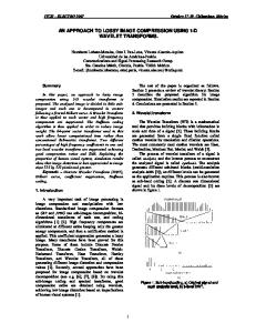
Figure 1: Typical CT images a) Image A (abdomen), b) Image B (pelvic region), c) Image C (lung), d) Image D (lung), e) Image E (kidney). Image A-D are from GE scanner and E from Philips scanner
2. DESCRIPTION OF METHOD The block diagram of encoder and decoder is shown in Fig. 2. In any compression method the image is first prediction or transform coded for energy compaction. The result is then entropy coded to obtain compression. The segmentationbased method will have an overhead of storing the shape information also. This method will be useful if the number of bits required to store the shape information and number of bits required to store texture information of objects is less than the number of bits required to represent the whole image as a single frame. Our main focus was to study the compression ratio obtained by using the segmentation based technique. Initially the experiments were conducted by using manual segmentation followed by extension to the problem of automatic segmentation. Encoder
Image
Predictive coder
Object Extraction & Shape coding
Decoder
Entropy coder
Compressed Bit stream
Entrop y decode
New Additions
Predictio n decoder
Image
Shape decode r
Figure 2: Image Compression Encoder and Decoder
Proc. of SPIE Vol. 5371
161
2.1 Segmentation Segmentation has long been an area of research in Medical Imaging. The segmentation techniques are application specific. The histogram plot of Image A is shown in Fig. 3. It can be seen from the histogram that the intensities of pixels fall into three regions. This property can be exploited for segmentation. Automatic segmentation is done based on thresholding. A binary image is formed with the value of pixel being one if the intensity of the pixel is greater than the threshold value and the rest of the binary image is chosen as zero. By choosing the threshold value 900 the binary image for anatomically relevant region (ARR) as shown in Fig. 4a is obtained. By choosing threshold as 0 we obtain the binary mask for the Field of View (FOV). For CT images this technique is particularly useful as each tissue is characterized by particular intensity range in Hounsfield unit.
Figure 3: Histogram of Image A
(a)
(b)
(c)
Figure 4: a) Binary image obtained by thresholding at 900 (Image A). Intensity above threshold is shown as white and below threshold is shown as black. b) Contour of the anatomically important region (ARR) from (a), c) Binary mask generated by filling the contour of (b).
By traversing along the boundaries of regions that are obtained after thresholding, the contours are obtained as shown in Fig. 4b. In this method care has been taken to exclude the support table form the anatomically relevant region. The contours obtained are filled to get the binary masks for the objects (Fig. 4c). These binary masks are used to separate the regions. The binary mask for Field of view (FOV) is obtained in the same way as done above for the anatomically relevant region. The final segmented image is shown in Fig. 5.
162
Proc. of SPIE Vol. 5371
Figure 5: Segmented Image where black region shows background (i.e. outside field of view). The part within field of view is divided into anatomically relevant region (ARR) and anatomically irrelevant region (AIR) shown in white and gray respectively.
2.2 Shape Coding Once the segmentation is done the shape information has to be stored. The shape information can be stored by contour methods like chain coding, polygonal approximations, Fourier descriptors or the region based method like quad tree method. The polygonal approximations and Fourier descriptors are lossy shape coding techniques whereas chain code and quad tree are lossless techniques. As medical images require lossless compression, polygonal approximations and Fourier descriptors are not considered for shape coding. In terms of coding and decoding complexity and coding efficiency chain code is much better than the quad tree method for lossless coding. Hence chain coding is used for shape coding [2]. 2.2.1 Chain coding The most popular chain codes are the 4-connected and the 8-connected chain codes. We used the 8-connectivity chain code is used for contour coding. The starting point of each contour is stored. The chain code is represented as C= {ci | i=1, 2, 3…N} where, ci is a link according to 8-directional chain code and N is the number of links 3
4
2
1
0
5 6: 8-connected chain code 7 Figure 6 Let ei=ci-ci-1 di=
ei+8 ei<-3 ei-8 ei>4 ei else
The differential chain code D= {di|i=1, 2, 3…N} where di is given by the above equation. D is Huffman coded for compression. The differential chain code depends only on change in direction. Huffman coding of differential chain code results in average bits of 1.3 –2 bits per chain link. The chain code can be obtained from differential chain code by ei =mod (di+8, 8) and ci=ei+ei-1
Proc. of SPIE Vol. 5371
163
2.3 Prediction Coding Once the shape information is stored the texture information of objects has to be stored. A simple 1D-DPCM is used as the prediction coder. The prediction residual e(i)=a(i)-a(i-1) is found and these residuals are entropy coded to obtain compression. The image frame is read in raster scan order into a single dimensional array and 1D-DPCM is used on this single dimensional array. When the image is segmented into objects each object is scanned in raster scan order and stored into a single dimensional array. The prediction residuals array obtained after DPCM is also single dimensional array. Fig. 7 shows the Image A after DPCM.
Figure 7: Image after DPCM
2.4 Entropy Coding The 1st order entropy is estimated for each object and for the whole frame as it gives an idea of the best compression that can be achieved with the particular coder used. Entropy is the average bits per pixel required to represent the image. The experiments are conducted to find the number of bits required to represent the whole frame and number of bits required to represent the when it is segmented into 2 objects and 3 objects. When an image is segmented into objects the total number of bits required to represent the image are: Total Bits = enti*Ni+ shape information, where enti and Ni are entropy and number of pixels for i-th segment. Effective Entropy = Total Bits/Total number of pixels 2.4.1 Huffman Coding Entropy gives an estimate of the best compression that can be achieved. In practice the entropy coder tries to touch this limit. To have actual bit rate (bits/pixel) the prediction error symbols are Huffman coded similar to the coding of DC coefficients in JPEG. The error symbols are represented in size/amplitude form. Only size is Huffman coded. Each Huffman code is followed by number of bits equal to size, which represent the amplitude [3]. The Huffman table overhead for each region is negligible; hence they are not included in the estimate for the number of bits.
3. SIMULATION AND RESULTS Simulation is performed following the method described in previous section. The image divided up to four objects. Fig. 8 shows the way in which images were divided into objects. Simulations for image segmented into four objects are done only on manually segmented images. The results of entropy estimates are shown in Tables 1 and 2. We observe that there is a reduction of about 11 to 13% in entropy. We also observe that there is not much change in percentage improvement by increasing the number of objects from Tables 1 and 2. It can be observed that the entropy of the background is very low (0.000309). The bits/pixel estimates using Huffman coding are shown in Tables 5 and 6 (Appendix). The percentage reduction in bits/pixel reduced to 7%-9%. This is because for Huffman coding the no. of bits/pixel in the background is now at least 1 bit/pixel where as the entropy was very low (0.000309 bits/pixel). We would have obtained better results if we had used run-length coder or arithmetic coder in the background.
164
Proc. of SPIE Vol. 5371
(a)
(b)
(c)
(d)
Figure 8: For Image C a). original image (single object) and b), c) and d) shows the masks for two, three and four object representation respectively.
Total Frame
Background
Field of view(FOV)
Images A B C D E
Ent. 5.2941 5.6902 5.5144 6.0882 5.0242
Pixels 262144 262144 262144 262144 262144
Ent. 0.000309 0.000309 0.000309 0.000309 0.000309
Pixels 55772 55772 55772 55772 55772
Ent. 5.9286 6.3936 6.2136 6.8449 5.6388
Pixels 206372 206372 206372 206372 206372
Chain code 2560 2560 2560 2560 2560
Segmentation Method Effective Ent. 4.6673 5.0334 4.8917 5.3887 4.4392
% Improvement 11.65% 11.37% 11.12% 11.33% 11.45%
Table 1: Entropy estimate when image is divided into two objects
Anatomically Irrelevant Region
Background
Anatomically Relevant Region
Images
A B C D E
Ent. 0.000309 0.000309 0.000309 0.000309 0.000309
Pixels 55772 55772 55772 55772 55772
Ent. 5.2276 5.5654 5.1825 6.7014 5.0148
Pixels 85236 81573 81195 19380 82697
Chain code 2560 2560 2560 2560 2560
Ent. 6.3194 6.836 6.7355 6.8562 5.9473
Pixels 121046 124799 125117 186992 123675
Chain code 1958 2280 1965 2314 2022
Segmentation Method % Effective Improvem Ent. -ent 4.6178 12.45% 4.9863 12.05% 4.8200 12.28% 5.3861 11.23% 4.3879 12.32%
Table 2: Entropy estimate when image is divided into three objects
The ARR of Image C is divided into the lung region and ARR outside lung region. The same way all the images are divided further. Fig. 9 and Fig. 10 shows the estimated bit budget and percentage savings with respect to number of objects used for compression calculated using entropy estimate. Fig. 11 and .Fig. 12 show the same statistics while compression is performed using Huffman coding.
Proc. of SPIE Vol. 5371
165
Estm. Bit budget (bytes)
1,700,000 1,600,000
Image A
1,500,000
Image B
1,400,000
Image C
1,300,000
Image D Image E
1,200,000 1,100,000 One Object
Two Three Four Objects Objects Objects
Estm. Bit budget savings (%)
Figure 9: Plot of bit budget based on entropy estimate vs. number of objects used for compression
13.00% 12.50%
Image A
12.00%
Image B
11.50%
Image C Image D
11.00%
Image E
10.50% 10.00% Two Objects
Three Objects
Four Objects
Figure 10: Plot of percentage savings in estimated bit budget vs. number of objects used for compression
Bit budget (bytes)
1800000 Image A
1600000
Image B 1400000
Image C Image D
1200000
Image E
1000000 One Object
Two Objects
Three Objects
Four Objects
Figure 11: Plot of bit budget using Huffman coding vs. number of objects used for compression
166
Proc. of SPIE Vol. 5371
Bit budget savings (%)
10.00% Image A
9.00%
Image B
8.00%
Image C 7.00%
Image D
6.00%
Image E
5.00% Tw o Objects
Three Objects
Four Objects
Figure 12: Plot of percentage savings in bit budget using Huffman coding vs. number of objects used for compression
We observe in Fig. 7 that the background is uniformly zero. When the image is divided into two regions the probability of occurrence of symbol zero increases in background. Hence the code length of zero decreases in the background resulting in reduction of number of bits in background. Also the probability of occurrence of zero decreases in Field of view (FOV), which means probability of occurrence of other symbols increase in FOV resulting in further reduction of number of bits. The probability of occurrence of symbol zero is approximately same in both anatomically relevant and irrelevant regions. Dividing the field of view (FOV) into anatomically relevant and irrelevant parts did not result in appreciable decrement of entropy. Hence there is a high percentage reduction when image is divided into 2 objects where as the percentage reduction almost remains same as we divide the image into three objects. 3.1 Progressive Decoding We have seen in the previous section that division of image into more than two regions does not decrease the effective entropy when compared to division of image into two regions. But division of image into more regions has the advantage of progressive decoding. For diagnostic purposes only the anatomically relevant region is important. Hence in client-server application initially only the anatomically relevant part can be decoded at the client end, followed by FOV and if needed the whole image can be decoded. From progressive decoding/transmission point of view decoding of only ARR is equivalent to deleting other segments. The same logic holds true for progressive transmission/decompression of FOV. The corresponding gains are shown in Table 3. For progressive decoding of FOV the gain is about 11%, while the same for ARR can go up to 45%. This means if only ARR needs to be transmitted for diagnostic purposes it takes about half the time that would be required to transmit the whole image. It is also noted that the gain in progressive decoding of ARR highly depends on the size of ARR.
Images A B C D E
% Saving in bit budget for decoding only FOV 11.53% 11.96% 10.88% 11.77% 11.49%
% Saving in bit budget for decoding only ARR 44.88% 42.89% 41.70% 19.89% 43.95%
Table 3: Bit budget savings for decoding only FOV and ARR. The results reported are bit rate achieved by Huffman coding.
Proc. of SPIE Vol. 5371
167
3.2 Boundary Extension In the previous section we have noticed that decoding only the anatomically significant region (ARR) leads to a huge saving for transmission. However, such method makes the system highly dependent on the accuracy of the segmentation. One way to address this problem is to make it apparent to the user whether the segmentation scheme has faithfully captured the ARR. For this purpose the boundary of anatomically relevant region is extended by few pixels. The advantage of this is that the radiologists will be sure that the segmentation did not result in deletion of any anatomically relevant region. Fig 13 shows how the contour is expanded. The results of segmentation based compression on normal boundaries and with extended boundaries are shown in Table 4. It shows that extension of boundary does not change the compression gain.
(a)
(b)
Figure 13: For Image A (a) regular and extended contour and b) anatomically relevant region for extended contour
Images A B C D E
% Savings in bit budget using original boundary 8.47% 8.60% 8.34% 8.18% 7.94%
% Savings in bit budget using extended boundary 8.46% 8.78% 8.24% 8.21% 7.88%
Table 4: Savings in bit budget (for 3 objects) when original ARR boundary is used and the case when extended ARR boundary is used. The results reported are bit rate achieved by Huffman coding.
3.3 Interpolation The CT images that are obtained by scanners are 512x512 resolution images. For display of images on big screens for example in classrooms or in medical theaters we need high-resolution images. We need high-resolution images like 1024x1024 or 2048x2048 images from 512x512 images. Interpolation is done to obtain high-resolution images. By using segmentation based interpolation we can obtain better high-resolution images [4].
4. DISCUSSION AND CONCLUSIONS In comparison to compression of the image as a single frame the segmentation based encoder performs better. The segmentation-based compression produces about 7%-8% better lossless compression than the normal compression scheme. Dividing the image into more than two objects does not help much to increase the compression gain. However, meaning objects generation can improve the progressive decoding to a great extent. Dividing the CT image into anatomically relevant region and otherwise is one such example. For diagnostic purposes if only diagnostically relevant
168
Proc. of SPIE Vol. 5371
information is to be decoded this can be done in this method and this results in reduction of total number of bits by about 45%.As the diagnostically relevant information is separated from diagnostically irrelevant information the diagnostically irrelevant regions can be coded using lossy compression methods. This will result in better compression. This opens up new ways to handle huge amount of data. If the law of the country permits lossy compression for medical application, by deleting the segments other than anatomically relevant region, data archive can also get the same benefit as progressive decoding. Better interpolation for segment based coding comes as an auxiliary benefit to this proposed scheme. Acknowledgement We would like to thank all the members of ImT Lab at John F. Welch Technology Centre for their valuable help and support in the project. References 1. Erickson BJ , Manduca A, Palisson P, etal. “Wavelet Compression of Medical Images”, Radiology, 1998, vol. 206, pp 599-607 2. Lu C.-C.; Dunham J.G, “Highly efficient coding schemes for contour lines based on chain code representations.”; IEEE Transactions on Communications, Volume: 39 Issue: 10 , Oct. 1991Page(s): 1511 -1514. 3. Bhaskaran Vasudev, Konstantinides Konstantinos, Image and Video Compression Standards, Algorithms and Architectures (second edition), Chapter 5, Kluwer Academic Publishers, 1997. 4. Ratakonda K. and Ahuja N, “POCS-Based Adaptive Image Magnification” , Proc. International Conference on Image Processing, Vol 3, Chicago, IL, October 1998, pg 203-207
5. APPENDIX Total Frame
Background
Field of view(FOV)
Images A B C D E
Bits/pixel 5.3851 5.8000 5.5971 6.2069 5.1011
pixels 262144 262144 262144 262144 262144
Bits/pixel 1.000197 1.000197 1.000197 1.000197 1.000197
pixels 55772 55772 55772 55772 55772
Bits/pixel 6.0387 6.4736 6.3231 6.9434 5.7247
pixels 206372 206372 206372 206372 206372
Chain code 2560 2560 2560 2560 2560
Segmentation Method Effective Bits/pixel 4.9765 5.3189 5.2004 5.6887 4.7293
% improvement 7.59% 8.30% 7.09% 8.35% 7.29%
Table 5: Bits/pixel estimate when image is divided into two objects using Huffman coding
Imag es A B C D E
Background
Bits/pixel 1.000197 1.000197 1.000197 1.000197 1.000197
Pixels 55772 55772 55772 55772 55772
Anatomically Irrelevant Region
Bits/pixel 5.347 5.6795 5.2922 6.8343 5.1199
Pixels 85236 81573 81195 19380 82697
Chain code 2560 2560 2560 2560 2560
Anatomically Relevant Region
Bits/pixel 6.4066 6.9344 6.8294 6.9543 6.0455
pixels 121046 124799 125117 186992 123675
Chain code 1958 2280 1965 2314 2022
Segmentation Method % Effective improv Bits/pixel ement 4.9269 8.51% 5.2998 8.62% 5.1288 8.37% 5.6973 8.21% 4.6976 7.91%
Table 6: Bits/pixel estimate when image is divided into three objects using Huffman coding
Proc. of SPIE Vol. 5371
169