JOURNALOF

Monetary ELSEVIER

Journal of Monetary Economics 36 (1995) 269-300

ECONOMICS

Search in the labor market and the real business cycle Monika Merz Department of Economics, Rice University, Houston, TX 77005-1892, USA (Received January 1993; final version received September 1995)

Abstract Existing models of the business cycle have been incapable of explaining many of the stylized facts that characterize the US labor market. The standard real business cycle model is modified by introducing two-sided search in the labor market as an economic mechanism that propagates technology shocks. This new analytical environment can explain many phenomena of the business cycle that the standard model either has resolved in an unsatisfactory manner or has not been able to address at all.

Key words: General equilibrium; U n e m p l o y m e n t and wages; Business cycles JEL classification: D51; E24; E32

What we mean, in ordinary usage, by 'unemployment' is exactly disruptions in, or difficulties in forming, employer-employee relationships. Simply hamstringing the auctioneer in a Walrasian framework that assigns no role at all to such a relationship is not going to give us the understanding we want. If we are serious about obtaining a theory of unemployment, we want a theory about unemployed people, not unemployed 'hours of labor services'; about people who look for jobs, hold them, lose them, people with all the attendant feeling that go along with these events. Walras' powerfully simple scenario, at least with the most obvious choice of 'commodity space' cannot give us this, with cleared markets or without them. R.E. Lucas, Jr. (1987, p. 53) This paper is based on Chapter 1 of my doctoral dissertation written at Northwestern University. I am deeply indebted to Lawrence Christiano and Dale Mortensen for their guidance. Useful comments on earlier drafts were made by Martin Eichenbaum, by participants at the NBER Economic Fluctuations Small Group Workshop in Micro and Macro Perspectives on the Aggregate Labor Market in Palo Alto in February 1993, by participants at the 9th Annual Congress of the European Economic Association in Maastricht in September 1994, and by seminar participants at Northwestern University. 0304-3932/95/$09.50 © 1995 Elsevier Science B.V. All rights reserved SSDI 0 3 0 4 3 9 3 2 9 5 0 1 2 1 6 B

270

M. Merz / Journal o f Monetary Economics 36 (1995) 269-300

1. Introduction

The macroeconomic performance of the US labor market is often described by stylized facts that express key empirical characteristics of this market. Labor productivity is more volatile than real wages, and it functions as a leading indicator of employment over the business cycle. With wages fluctuating relatively little, labor's share of total income behaves countercyclically. Furthermore, unemployment is negatively correlated with job vacancies, and both unemployment and employment exhibit a high degree of persistence. Employment is more volatile than real wages. These observations pose a major challenge for the standard neoclassical growth model, often referred to as the real business cycle (RBC) model, that was pioneered by the work of Kydland and Prescott (1982) and Long and Plosser (1983). It tends to perform well in explaining much of the empirically observed behavior of aggregate variables such as output, private consumption, investment, and capital stock over time. However, this model fails to capture many of the stylized facts that characterize the labor market. In its original version, it focuses on the intertemporal substitution between leisure and employment, ignoring the issue of unemployment altogether. It views the labor market as frictionless and run by a Walrasian auctioneer, so that there is no room for unfilled job-vacancies. With wages equalling the marginal product of labor and a constant-returns-to-scale production process it generates a constant labor's share of income. The model also fails to match the actual behavior of the dynamic correlation between employment and productivity in that it overstates their contemporaneous correlation, and that it cannot predict the fact that productivity leads hours over the cycle. Technology shocks, as its sole driving process, shift the demand curve for labor, thereby tracing out a constant labor supply function. Hence, the model predicts the contemporaneous correlation between these variables to be close to one and higher than any of the correlations at leads or lags. When introducing unemployment via a lottery system into the standard model, Hansen (1985) and Rogerson (1988) improve the relative volatility of employment to real wages, but unemployment, employment, and output exhibit too little persistence. In this paper I replace the frictionless Walrasian-style labor market by one in which trade frictions are present, thereby creating a synthesis between the stochastic neoclassical growth model and the transactions cost approach to unemployment. Pissarides (1988) introduced this approach into the literature. It views the labor market as characterized by two-sided search. Its two distinctive features are search externalities, acting as main propagation mechanism of shocks, and a theory of wage determination. Search externalities arise since the rate at which searching workers and firms make job contracts depends on the tightness of the labor market, that is, the relative number of traders on both sides of the market. Furthermore, an explicit theory of how to determine the

M. Merz /Journal of Monetary Economics 36 (1995) 269-300

271

wage for a newly created job match is required since such a match generates a surplus over which the worker and the firm involved need to bargain. The transactions cost approach to unemployment has grown out of the theory of search in the labor market as formulated by Phelps et al. (1970) and has subsequently been used by Pissarides (1990), Blanchard and Diamond (1990, 1989), and Mortensen (1992), for example, to study aggregate phenomena of the labor market. It has generated a consistent equilibrium dynamic theory of unemployment, job vacancies and wage formation, but the dynamic interaction between the labor market and other markets in the economy has rarely been studied. My goal in this paper is to quantitatively test the qualitative implications that the transcations cost approach to u n e m p l o y m e n t - and thus search theory has for aggregate economic variables, thereby assessing the theory's contribution to explaining certain phenomena of the business cycle that the standard neoclassical growth model either has resolved in an unsatisfactory manner or has not been able to address at all.~ I show that, when trade frictions are present, the equilibrium real wage deviates from labor productivity. This result has important implications for the dynamic behavior of many labor market variables. Real wages are less volatile than labor productivity which implies that labor's share of income behaves countercyclically. Moreover, since matching takes time, productivity leads employment over the cycle. When unemployed workers search at a constant intensity, any increase in vacancies leads to matching and a consequent drop in the unemployment rate which is reflected by their negative contemporaneous correlation. Finally, trade frictions in the labor market introduce history dependence for any state within the labor force which, compared to Hansen's (1985) indivisible labor framework, increases the degree of persistence of employment, unemployment, as well as of aggregate output. This paper is organized as follows. In Section 2 I formulate the social planner's version of my model economy and derive the first-order necessary conditions for an optimum. In Section 3 I describe how I choose the parameters used to calibrate the model. Section 4 presents and discusses the simulation results, and in Section 5 I draw the conclusion of the analysis and point out possible applications of the new analytical environment.

2. The model

The economy to be studied is populated by a continuum of identical infinitely lived worker-households with names on the closed interval [0, 1], and a

~ln an independent line of research, Andolfatto (1993) also studies quantitative implications of search environmentsin a general equilibrium setting.

272

~ Merz / Journal of Monetary Economies 36 (1995) 269 300

continuum of identical competitive firms. Each household is thought of as a very large extended family which contains a continuum of members. Members in each family perfectly insure each other against variations in labor income due to employment or unemployment. Households and firms interact in both the exchange of goods and factors of production. While goods and the factor capital are exchanged in perfectly competitive markets, labor is traded in a process that exhibits search externalities for individual households and firms. Search externalities arise, since trade frictions are present in the process in which households and firms exchange the factor labor. The rate at which searching workers and firms make job contacts depends on the tightness of the labor market, that is, the relative number of traders present on both sides of the market. For any given trader, a positive externality arises whenever the number of traders on the opposite side of the market increases. With the increased market thickness, a profitable trade becomes more likely for her. Similarly, a negative externality arises whenever the number of agents on the same side of the market increases. This situation is referred to as congestion, since it makes trade more difficult. Creating new job matches comes at an expense, since it requires firms to post vacancies in order to recruit applicants, and since unemployed workers need to search with a variable intensity for a suitable job. Both kinds of search activity take time and other real resources. Finally, job matches are assumed to be dissolved with an exogenously determined probability every period. In what follows, I present the social planner's version of my model economy. It specifies preferences, technologies, constraints, the stochastic environment, as well as the information structure of the aggregate economy. For a static economic environment in which search externalities are present and labor is the sole input into the production process, Hosios (1990) has worked out the conditions under which the solution to the welfare-maximizing problem can be decentralized as a market equilibrium. They correspond to setting incentives for traders on both sides of a search market such that all positive and negative externalities just offset one another. I extend this result to a dynamic environment with both labor and capital entering the production function. In Appendix A I spell out a corresponding market structure with firms' and households' optimization problems as well as the factor prices and matching rates that support the Pareto optimal outcome of the social planner's problem as a recursive competitive equilibrium.

2.1. The social planning problem The labor force in my model economy is constant and normalized to one. This assumption helps focusing the analysis of the labor market on the margin that seems most relevant when studying search unemployment: the transition between unemployment and employment. The analysis thus abstracts from any transition between in and out of the labor force. The time series of the beginning-

M. Merz /Journal o f Monetary Economics 36 (1995) 269-300

273

of-period-t per capita stock of capital (Kt), private time-t consumption (Ct), total employment (Nt), total unemployment (1 - Nt), search intensity (St), and job vacancies posted per firm (Vt) are taken as the outcome of the following welfare maximization problem. The social planner evaluates streams of consumption services (Ct) and employment (Nt) according to the objective function Eo ~. fl'U(C. Nt),

0
(1.1)

t--O

with preferences of the representative household specified as

U (Ct, Nt) = U (Ct) - G( Nt).

(1.2)

The parameter fl denotes the common discount factor in the economy, and both U and G represent increasing and concave functions in their respective argument:

U(Ct) = log(Ct),

G(Nt) = N1-1/"/(1 -- l/v).

(1.3)

The parameter v measures the negative of the Frisch elasticity of labor supply which is defined as the wage elasticity of labor supply at a constant marginal utility of wealth. The representative household can be thought of as consisting of a very large number of members who pool their income and, thus, provide each other with complete insurance against unemployment. Aggregate per capita output, Yt, can either be consumed, invested, or spent on search activity. That is, when varying search intensity, a cost per unemployed worker, c(St), is incurred, which is measured in terms of the single output good in the economy. Similarly, posting a vacancy comes at a constant advertising cost, a. Hence, the aggregate resource constraint of the economy must be satisfied:

C~ + It + exp(Itt)c(St)(1 - Nt) + exp(la)aVt <~ Yt.

(1.4)

The search cost function is assumed to be of the form c(S,) = coS7, with Co > 0, q > 1, and St >>-O. It can be thought of as representing some kind of shoe leather cost that increases with an increase in search intensity. The parameter/a >~ 0 denotes the rate at which all variables in the economy grow over time, except for search intensity, vacancies, employment, and unemployment, which are stationary. Thus, the model exhibits balanced growth. Aggregate per capita output is produced, using the constant returns to scale technology that is given by

Y t = f ( z t , Kt, N t ) = e x p [ ( 1 - ~ ) ( p t + z t ) ] K ~ N ~ t

~,

0 ~ < ~ < 1,

(1.5)

where accumulated capital and employment are the inputs and exp([1 - ~.)x (#t + zt)] denotes labor-augmenting technical progress. The technology shock zt is assumed to follow an AR(1) process with the following law of motion: Zt+ 1 = Pzt + £t+ 1,

0

< p < 1.

(1.6)

M. Merz / Journal of Monetary Economics 36 (1995) 269-300

274

Here ~t is an i.i.d, random variable drawn from a normal distribution with mean zero and standard deviation G. The per capita capital stock depreciates at the constant rate 6 in each period and is augmented by any investment undertaken. Thus, it obeys the following law of motion:

Kt+ a = (1

-

6)K t

+ It,

0 _< 3 _< 1.

(1.7)

Similarly, aggregate employment evolves according to Nt+

1 =

(1

--

~O)N, + Mr,

0 < ff < 1,

(1.8)

where Mt represents the number of job matches that are created in time period t. In fact, job matches can be thought of as being generated by a standard Cobb-Douglas production function of the form Mt

=

vtl-)[gt(1

--

Nt)] a,

0 _< 2 < 1.

(1.9)

The assumption of this matching technology exhibiting constant returns to scale is consistent with the empirical findings reported by Blanchard and Diamond (1989) for US data and by Pissarides (1986) for the United Kingdom. It implies endogenous probabilities for the transition from unemployment to employment, Pt, and from an unfilled vacancy to a filled one, qt, that depend on the tightness of the labor market, Or, and the aggregate search intensity, St: Pt = Mr~St(1 - Nt) = (St-~0t) 1-~

where

0, = V,/(1 - N~),

(1.10)

q, = M t / V t = (S,O~- 1)z.

Furthermore, it implies that the probability of making a transition from unemployment to employment decreases with congestion caused by an increase in either the stock of unemployment or aggregate search intensity. This probability increases with an increase in market thickness brought about by an increase in the number of listed job vacancies. Of course, the opposite holds true for the probability of an unfilled vacancy to become filled. Total search effort defined as the product of aggregate search intensity and the stock of unemployment and recruiting are investment activities that may lead to the creation of new job matches, thereby helping augment the stock of aggregate employment. Hence, when leading to new job matches, both of these activities counteract the natural transition from employment to unemployment, which is assumed to be exogenous and to take place at a constant rate ft. Consequently, the social planning problem consists of the planner choosing contingency plans for {Ct, K , + I , N t + I , S , , gt: t >_ O} at time 0 in order to maximize the objective function (1.1) subject to (1.2)-(1.9), K o , and No. The social planner is assumed to make period t decisions based on all information available at time t. When a technology shock is observed in a period, investment in search and recruiting takes place in response. The new matches, together with the separations that occur during this period, determine the level of aggregate

M e r z / Journal o f M o n e t a r y Economics 36 (1995) 2 6 9 - 3 0 0

275

employment at the beginning of next period. Similarly, the planner decides upon the level of investment during the period in which she observes shocks. New investment adds to the existing capital stock, and, together with the newly created job matches, they become productive in the following period. Since the model exhibits balanced growth, all nonstationary variables have to be detrended in order for the model to be solvable by linear quadratic approximation around the stationary steady state. For that purpose, the detrended versions of the respective variables are defined as follows: /(,+1 = Kt+y/exp(#t),

Ct = C,/exp(pt),

T, = I,/exp(pt).

(1.11)

Assuming that, due to nonsatiation, the aggregate resource constraint is binding, (1.5) can be substituted into (1.4) so that the social welfare problem that includes only stationary variables can be summarized as the following dynamic programming problem: W(f2t) =

max {U(Ct, N t ) + f l E [ W ( f 2 t + l ) l f 2 t ] } , {L,v,,s,}~-o

subject to C = Y, - L -- c(St)(1 - N,) - aV,,

/~t+, = ( 1 - 6')/(, + fit, Nt+l : (1 -- O)N, + Mr, Zt + 1 = P Z t -[- •t + 1 ,

where g2t summarizes the aggregate state of the economy in time period t that consists of the exogenous state variable z,, the endogenous state variable Nt, and the detrended version of K,: at : { z , , g t , Nt}.

Furthermore 6' = 1 - (1 - c~)exp(- #) and 4' = e x p ( - ~#). W(.) stands for the optimal value function. Aggregate output Y, is produced according to the Cobb-Douglas production function described in Eq. (1.5), and job matches Mr are generated according to Eq. (1.9). The solution to this dynamic programming problem consists of the set of functions /(,+, = g(f2t),

N,+I = h(f2t).

(1.12)

The functions g and h are the decision rules according to which the social planner determines present and future values of all the variables in the artificial economy under study. Once g and h are determined, the model is solved. Given the nonlinear nature of the problem, in general, the decision rules g and h cannot be solved for analytically. However, they can be solved for using numerical methods. Alternatively, they can be approximated rather precisely by linearizing

M. Merz / Journal of Monetary Economics 36 (1995) 269-300

276

the Euler equations of the maximization problem around the stationary steady state and finding a unique solution to the resulting system of dynamic equations. This latter method, which is referred to as the state-space approach to linearization, is explained in detail in King, Plosser, and Rebelo (1987). I use this method to solve the model. 2.2. First-order necessary conditions and costates

The first-order necessary conditions and costates that correspond to the social planner's dynamic programming problem help shed some light on the planner's intertemporal allocation decisions. In particular, they nicely demonstrate the dynamic characteristics of aggregate employment in a framework with transactions cost in the labor market. L:

- ie,

I ,)

- o,

V,:

- aUe, + flE(WN,+I [f2t)Mv, = O,

St:

- Ue, cs,(1 - Nt) + flE(WN,+, I Or)Ms, = 0,

if.t:

~_R, + 1 Wg, = Uc,fg, + flE(Wg,+, lot) O/~t '

N,:

WN, = Ue,[fN, + c(St)] -- GN + flE(WN,+, I O,) eN,

~Nt+ l

where

~N,+ I ~Nt - (l - ~) - M1_ N,.

The law of motion for the capital stock as costate variable is standard. Combined with the first-order condition for capital investment it describes the planner's decision to optimally allocate consumption over time. According to the law of motion for aggregate employment, the marginal contribution to social welfare of a newly created job match equals the sum of its marginal product net of disutility arising from work and its discounted future contribution to social welfare if it is not dissolved in the meantime. It is dissolved with probability (1 - 0). This expected payoff needs to be corrected for future matching opportunities foregone since the stock of unemployment is reduced by a newly created match. Hence, this law of motion nicely demonstrates the fact that the degree of persistence of any job match - and thus of aggregate employment - depends on the assumed probability with which it survives a given period. Substituting the respective expectational expressions from the first-order necessary conditions into the latter two equations for the costates summarizes the Euler conditions

M. Merz / Journal of Monetary Economics"36 (1995) 269 300

277

for the social planner's dynamic programming problem: (Pl)

UC=flE{Uc+,[fg,+ , +(1-6,)31f2t

(P2)

aUC My, - fiE { UC+,[fN,,

},

+ c(S,+l)] - GN,+,

aUc+' 1

,

}

+ - ~ v , + E( - - O ) + M N , . 31(2, , (P3)

UCcs'(1 - N,) { Ms, ----fiE_Uc+~[fN.... + c ( S , + , ) ] - G v , + , Jr- Uet~lcs'+a(1Ms,+,-N'+

1) [(1 - 0) + MN,.,] ] Qt}

3. Model calibration To actually compute the decision rules in (1.12) and generate artificial time series, it is necessary to choose specific parameter values for ~, fl, 6, q, 0, ),/~, p, 0, a, Co, and a~. It has become a common procedure in the RBC literature to base these values on evidence from growth observations and micro studies. For the sake of comparability, I proceed in the same manner, building on existing studies as much as possible. Since the model presented here primarily aims at explaining the cyclical behavior of a selected set of labor market variables, I determine many parameter values such that the model's first moments of some of these variables coincide with their empirical counterpart. The parameters used for calibrating the model are summarized in Table 1. The parameter ~ corresponds to the elasticity of output with respect to capital. This has been calculated using US time series data by Kydland and Prescott (1982) and was found to be approximately 0.36. This elasticity coincides with the capital share of total income. However, since the wage rate in this model economy does not correspond to the marginal product of labor, (1 - :~) is not equal to the labor share of total income. (1 - :0 equals the sum of the labor share of total income and the return to investing in job search. Contrary to the standard neoclassical growth model in which labor's share of income is constant, the model with trade frictions in the labor market exhibits a labor share that varies over the business cycle, thereby mirroring this variable's behavior in the data. The rate of depreciation of capital, 6, is set equal to 0.022. Together with /~ = 0.004 which implies an annual growth rate of 1.6 percent - this amounts to an effective depreciation rate 6' of 10.4 percent per annum. The common discount factor, fl, is set equal to 0.99, implying a steady state annual rate of interest of 4 percent. Since the cyclical behavior of most of the labor

278

M. Merz / Journal of Monetary Economics 36 (1995) 269-300

Table 1 Parameter values used for calibration Symbol

Value

Symbol

Value

fl 6 r/ v 2

0.36 0.99 0.022 1 - 1.25 0.40

~k # a Co p a~

0.07 0.004 0.05 0.005 0.95 0.007

The parameter ~ denotes output's elasticity with respect to the capital stock, fl the discount rate, 6 the capital stock's depreciation rate, r/the parameter measuring the convexity of the search cost function, v the negative of the Frisch elasticity of labor supply, 2 the elasticity of job matches with respect to total search effort, qJ the transition rate from employment to unemployment, p the common growth rate, a the per unit advertising cost, Co the parameter measuring the level of the search costs, p the autocorrelation coefficient for the technology shock, and ~r the standard deviation of the innovation in the technology shocks.

m a r k e t variables u n d e r c o n s i d e r a t i o n is sensitive to the choice of the p a r a m e t e r v of the utility function, I s i m u l a t e the m o d e l for three different values of v. I set v e q u a l to - 0.5, - 1, o r - 1.25. These values are c h o s e n such t h a t the i m p l i e d F r i s c h elasticities of the l a b o r s u p p l y t a k e on a plausible value. T h e i m p l i e d elasticities fall within the b r o a d s p e c t r u m of values t h a t have been c a l c u l a t e d b a s e d on m i c r o e c o n o m i c o r m a c r o e c o n o m i c d a t a sets. T h e y range from 0.01 for s o m e m i c r o e c o n o m i c studies to 3.0 in r e p r e s e n t a t i v e m a c r o e c o n o m i c studies. 2 In Section 4.2 I r e p o r t the s i m u l a t i o n results for the case when v equals - 1.25 a n d discuss the i m p l i c a t i o n s that v a r y i n g this value has on the cyclical b e h a v i o r of selected l a b o r m a r k e t variables. B l a n c h a r d a n d D i a m o n d (1989) p r o v i d e the only e m p i r i c a l s t u d y of the m a t c h i n g t e c h n o l o g y a v a i l a b l e for the U S with a g g r e g a t e vacancies a n d u n e m p l o y m e n t serving as the inputs. T h e i r results s u p p o r t the c o n s t a n t returns to scale specification. T h e e s t i m a t e d m a t c h i n g elasticities with respect to u n e m p l o y m e n t a n d vacancies equal 0.4 a n d 0.6, respectively. T o the extent that total search effort can be r e g a r d e d as the a p p r o p r i a t e m e a s u r e of u n e m p l o y m e n t in the m o d e l p r e s e n t e d above, these results s u p p o r t the a s s u m p t i o n of 2 = 0.4. T h e q u a r t e r l y rate of t r a n s i t i o n from e m p l o y m e n t to u n e m p l o y m e n t , also referred to as u n e m p l o y m e n t incidence, is c h o s e n to be ~k = 0.07. It equals the r a t i o of the u n e m p l o y m e n t rate to the e m p l o y m e n t rate. F o r the time p e r i o d r a n g i n g from

2Studies based on microeconomic data are the ones by Altonji (1986, 1982), Ashenfelter (1984), and McCurdy (1981). Studies of macroeconomic data were performed by Christiano and Eichenbaum (1992) and Rotemberg and Woodford (1991), for example.

M. Merz / Journal of Monetary Economics 36 (1995) 269-300

279

the first quarter of 1959 to the second quarter of 1988, the US unemployment rate is 6.1 percent. Hence, 0.07 = 0.061/(1 - 0.061). Alternatively, this ratio can be expressed as the product of unemployment incidence and unemployment duration, with duration being measured as the stock of unemployment relative to newly created job matches in a period. Jackman, Layard, and Nickell (1991) report that, on average, workers remain unemployed for one quarter before they become employed. Taken together, this evidence also implies a quarterly rate of transition from employment to unemployment of 0.07. I determine the parameters that describe firms' recruiting costs and workers' search costs by matching first moments of appropriately selected labor market variables with their model equivalent in steady state. I choose the per unit advertising cost, a, equal to 0.05 so that my model matches the rate of average vacancy duration that van Ours and Ridder (1992) report to equal 0.50, or 45 days, for the Dutch economy. This rate corresponds to the ratio between posted vacancies and newly created job matches. It expresses the average time it takes to fill a vacancy with a new hire which tends to be longer than the time it takes to select a suitable applicant for a position out of the pool of all applicants. Similarly, ! choose the level of a worker's search cost, Co, and its degree of convexity, 7, such that my model matches the average unemployment rate and unemployment duration for the time period considered. Setting Co equal to 0.005 and tt equal to 1 generates an average unemployment rate of 6.1 percent and an unemployment duration of one quarter. Finally, I parameterize the law of motion for the technology shock by setting p equal to 0.95 and a~ equal to 0.007. These values correspond to the ones in Hansen (1985). They allow me to compare the volatility of the variables in my model economy to the volatility of the corresponding variables in Hansen's economy.

4. Simulations The major goal of this study is to evaluate the contribution of the search-theoretic framework as one possible alternative to explaining observed aggregate fluctuations. Towards this end, I generate selected time series for the business cycle from two different versions of the search model. One version has workers vary their search intensity, S, in reaction to a change in the economic environment (Variable S). The other one represents an extreme case of this former version with workers' search intensity being constant (Fixed S). It is generated when Co converges to zero and t/converges to infinity. I present the more general model to be able to generate the Beveridge curve - the negative relationship between vacancies and employment. Only if the search intensity is fixed can we expect the model to replicate this negative relationship, since otherwise it gets blurred by a variable search intensity shifting the Beveridge curve.

280

M. Merz / Journal o f Monetary Economics 36 (1995) 269-300

4.1. Simulation procedure Each model is simulated 100 times to obtain many samples of artificially generated time series. Each sample generated has the same number of periods (118) as the US time series used in this study. Their statistical properties can be compared to the ones computed for the respective US data. The time series on per capita output, private consumption, capital investment, and the capital stock (in 1987 dollars, if nominal) consist of quarterly data that were originally compiled by Christiano (1988) and more recently updated and made available by Jonas Fisher. These data are available for all series from the first quarter of 1959 until the second quarter of 1988. I provide a more detailed description of the data in Appendix B. Availability of these data determines the time period of my analysis. It covers the first quarter of 1959 until the second quarter of 1988. I construct the remaining series on aggregate employment, unemployment, average labor productivity, vacancies posted, labor's share of income, and a real wage rate from data that originate from the CITIBASE tape. I describe the original data and how I compile them into the desired series in Appendix B. Before summary statistics are calculated, all time series are logged, and deviations from trend are computed. Detrending is necessary because the models studied abstract from growth. I detrend the data using the HodrickPrescott filter, as introduced by Hodrick and Prescott (1980). When applying this filter, I set the parameter 2, which expresses the penalty on a time series' variation, equal to 1600. In a final step, I compute the statistical properties of the time series of both the US economy and the artificial economies. They are summarized by a set of standard deviations and correlation coefficients. In what follows, I report and interpret the outcome of simulating both model versions with the set of parameters that are described in Table 1. I also discuss the implications that varying the parameter v has. 4.2. Simulation results I summarize the results from simulating the model with variable search intensity (Variable S) and with constant search intensity (Fixed S) in Tables 2, 3, and 4. I complement these results by some impulse response functions which I report in Appendix C. For each variable considered, they express the percentage deviations from steady state in reaction to a one-standard-deviation positive shock to the technological innovation. The model performs well in generating the relative cyclical behavior of the variables that are related to the labor market, and also of the commonly reported aggregates such as private consumption, capital investment, and the capital stock. Moreover, it nicely mimics some of the noteworthy features that characterize the dynamic behavior of the labor market.

M. Merz /Journal o f Monetary Economics 36 (1995) 269-300

281

Table 2 Second moments from US and artificial economies

US data 59:1 88:2

Model variable S

Model fixed S

ac/a r

0.40 (0.032)

0.30 (0.025)

0.31 (0.025)

~rp/a~

0.68 (0.043)

0.70 (0.026)

0.74 (0.022}

a~/ay

2.39 (0.058)

2.97 (0.114)

2.91 (0.115)

C~w/a~.

0.37 (0.(138!

0.31 (0.017)

0.34 (0.021)

aK/ay

0.22 (0.026)

0.25 (0.038)

0.25 (0.030)

cr,/a~,

6.11 (0.403}

5.85 (0.300)

4.63 10.186)

aE/ay

0.54 (0.038)

0.42 (0.008)

0.36 (0.007)

~v/ay

7.31 (0.345}

4.68 (0.660)

6.38 ~0.600)

aLs/~Y

0.53 (0.045)

0.49 (0.041)

0.47 (0.037)

p(V, u)

- 0.95 (0.009)

0.32 (0.063)

-- 0.15 (0.109}

ay

1.87 (0.045)

1.12 (0.002t

1.07 (O.OOl)

Statistic

Statistic

US data 59:1 88:2

Model variable S

Model fixed S

Y denotes per capita output, C consumption, I capital investment, K capital stock, E employment, LS labor's share of total income, P average labor productivity, w real wage rate per person per hour. u unemployment rate, and V job vacancies, a~/ay denotes the ratio between the standard deviation of variable x and the standard deviation of variable y. a~ denotes the standard deviation of variable x. p(x, y) denotes the contemporaneous correlation coefficient between variable x and variable y. The US time series on per capita output, consumption, capital investment, and the capital stock are taken from a version of the data base in Christiano (1988) that was updated by Jonas Fisher. All other series are constructed from data that are taken from the CITIBASE tape. A more detailed description of the data is provided in Appendix B. All statistics are computed after detrending the logarithm of the data using the Hodrick Prescott filter. The standard deviations are sample means of statistics computed for each of 100 simulations. Each simulation consists of 118 periods. The numbers in parentheses are sample standard deviations of these statistics. For the US data, standard deviations are calculated using the generalized method of moments.

T a b l e 2 c o n t a i n s t h e often q u o t e d e m p i r i c a l o b s e r v a t i o n t h a t real w a g e s f l u c t u a t e m u c h less o v e r the b u s i n e s s cycle t h a n t h e a v e r a g e l a b o r p r o d u c t i v i t y . O n e c o m m o n e x p l a n a t i o n is the o n e of risk s h a r i n g t h a t is p r o v i d e d by D a n t h i n e a n d D o n a l d s o n (1989), for e x a m p l e . It states t h a t r i s k - n e u t r a l firms are w i l l i n g to c o n t r a c t r i s k - a v e r s e w o r k e r s at a w a g e r a t e t h a t is less v o l a t i l e t h a n l a b o r p r o d u c t i v i t y , t h e r e b y i m p l i c i t l y i n s u r i n g t h e m a g a i n s t a h i g h d e g r e e of v o l a t i l i t y of t h e i r l a b o r i n c o m e . T h e W a l r a s i a n s e t t i n g of the l a b o r m a r k e t in the s t a n d a r d n e o c l a s s i c a l g r o w t h m o d e l c a n n o t a c c o u n t for this o b s e r v a t i o n , since it g e n e r a t e s a n e q u i l i b r i u m w a g e r a t e t h a t c o r r e s p o n d s to the m a r g i n a l p r o d u c t of l a b o r , so t h a t b o t h v a r i a b l e s a r e e q u a l l y volatile. O n e o f t h e i m p o r t a n t i m p l i c a t i o n s of i n t r o d u c i n g t r a d e f r i c t i o n s in t h e l a b o r m a r k e t is t h e fact t h a t this n e o c l a s s i c a l o b s e r v a t i o n n o l o n g e r holds. C o n s e q u e n t l y , t h e v o l a t i l i t y of b o t h

282

M. Mere / Journal of Monetary Economics 36 (1995) 269-300

Table 3 Dynamic correlations for US and artificial economy

Statistic

- 3

- 2

- 1

0

1

2

3

I. Employment and average labor productivity US data 59:1-88:2

p(Et, Pt ~)

Model variable S

p(Et, P,-~)

-- 0.325 (0.097)

- 0.151 (0.118)

0.092 (0.111)

0.345 (0.104)

0.577 (0.095)

0.687 (0.102)

0.730 (0.114)

0.155 (0.137)

0.281 (0.130)

0.432 (0.118)

0.596 (0.103)

0.964 (0.011)

0.593 (0.077)

0.305 (0,090)

II. Output and labor's share of income US data 59:1-88:2

P(Yt, LSt-O

-0.005 (0.112)

-0.216 (0.108)

-0.481 (0.089)

-0.739 (0.060)

-0.782 (0.067)

-0.728 -0.610 (0.093) (0.110)

Model variable S

p(Y,,LSt-r)

- 0.337 (0.110)

- 0.514 (0.099)

- 0.736 (0.064)

- 0.768 (0.029)

-0.231 (0.117)

- 0.095 - 0.020 (0.105) (0.105)

(0.097)

-0.769 (0.072)

-0.928 (0.042)

-0.954 (0.009)

--0.824 (0.054)

-0.607 -0.357 (0.097) (0.120)

IIl. Vacancies and unemployment US data 59:1 88:2

p(V,,u,_O

-0.535

Model variable S

p(Vt, ut-~)

0.200 (0.090)

0.224 (0.080)

0.263 (0.061)

0.322 (0.063)

- 0.476 (0.038)

0.365 (0.067)

Model fixed S

p(Vt, ut-O

0.094 (0.085)

0.035 (0.083)

- 0.045 (0.099)

- 0.153 (0.110)

- 0.824 (0.013)

0.590 - 0.400 (0.079) (0.100)

0.197 (0.090)

See Table 2. p(xt, Y,-O denotes the correlation between variable x and the rth lag of variable y ifr is positive, and between x and the rth lead of a variable y if r is negative.

variables cannot be expected to be the same either. According to Table 2, both versions of the search model generate the observation that real wages fluctuate less relative to aggregate output than does the average labor productivity. The search environment with the possible interpretation of the equilibrium wage as the outcome of a bilateral bargaining game thus provides an alternative explanation for this empirical observation without explicitly relying on the assumption of risk sharing. When firms and workers negotiate wages that take into account the marginal product of labor, and also components of search costs and utility foregone due to employment, workers become implicitly insured against labor income fluctuating as much as labor productivity. The first part of Table 3 demonstrates the dynamic behavior between employment and the average labor productivity. It captures the well-known empirical phenomenon that, over the business cycle, average labor productivity leads

M. Merz / Journal of Monetary Economics 36 (1995) 269-300

283

Table 4 Autocorrelations for US and artificial economy

Statistic

0

1

2

3

US data 59:1 88:2

p(ut, ut-~)

1.000 (0)

0.899 (0.041)

0.687 (0.078)

0.427 (0.107)

Model fixed S

p(ut, ut ~)

1.000 (0)

0.682 (0.073)

0.424 (0.110)

0.226 (0.123)

US data 59:1 88:2

P(Y,, Yt-~)

1.000 (0)

0.874 (0.049)

0.681 (0.078)

0.464 (0.093)

Model fixed S

P(Yt, Y~-~)

1.000 (0)

0.781 (0.051 )

0.500 (0.102)

0.278 (0.124)

I. Unemployment

II.

Output

See Table 3.

employment by two to three quarters. Again, with a Walrasian setting of the labor market the standard neoclassical growth model cannot account for this observation. A shock to aggregate technology - which can be interpreted as causing a shift of labor demand along a constant labor supply function - affects labor productivity and employment during one and the same period, thereby leading to a strongly positive contemporaneous correlation between these two variables. This shortcoming of the standard model is documented in Christiano and Eichenbaum (1992), for example. When trade frictions in the labor market are present, the growth model can generate the phenomenon that labor productivity leads employment. As can be seen in Fig. la of Appendix C, a positive technology shock immediately increases labor productivity, the number of posted vacancies, and aggregate search intensity. This translates into an increase in the number of job matches and a reduction of total unemployment. All new job matches are assumed to become productive in the following period. Hence, this model suggests a possible explanation for the dynamic correlation between employment and labor productivity. The time that elapses between an increase in labor productivity and a subsequent increase in employment can be interpreted as being required for creating new job matches and possibly training on the job - before they can become productive. According to Tables 2 and 3, labor's share of total income fluctuates about half as much as aggregate output. Furthermore, as is stressed by its negative correlation with output at various leads and lags, the labor share behaves strongly countercyclically. This latter observation can be easily interpreted

284

M. Merz / Journal of Monetary Economics 36 (1995) 269-300

when seen in connection with a real wage that fluctuates much less than average labor productivity. In an economic upswing, capital, managerial skills, and land bear the brunt of additionally created income, leaving the factor labor with a less than proportionate increase in income. The opposite holds true in a recession. The standard neoclassical growth model cannot account for either of these observations. As is well-known, when factor prices equal the marginal product of their respective input variable into a production process that exhibits constant returns to scale, each input variable receives a constant share of income. In the case of a Cobb-Douglas production function where ~ represents the elasticity of output with respect to capital, and (1 - ~) the elasticity with respect to labor, this latter elasticity corresponds to the labor share of income. When trade frictions are present in the labor market, this one-to-one correspondence no longer exists, since the real wage deviates from the marginal product of labor. Even though c~still represents capital's fixed share of income, (1 - ~) measures the sum of labor's share and the return to total search effort. Hence, the model with trade frictions correctly predicts the labor share to fluctuate over the cycle. In fact, labor share's implied relative volatility closely resembles its empirical counterpart. With real wages that fluctuate much less than average labor productivity, the model also correctly predicts the strong countercyclicality of labor's share of income. According to Table 2, unemployment and vacancies fluctuate by far the most among all labor market variables considered. Furthermore, they exhibit a strongly negative contemporaneous correlation - a phenomenon which has been labelled the Beveridge curve in recognition of the work of W.H. Beveridge. The growth model with trade frictions in the labor market provides one possible economic environment to study these phenomena. The overall degree of relative volatility that it generates, however, depends on the exact model specification. As the impulse response functions in Appendix C show, it increases with the degree of flexibility of the aggregate search intensity. The explanation for this observation lies in the specifics of the matching process. It takes both job vacancies and search effort to generate new job matches. An increase in one of these components can only lead to an increase in the number of matches if its impact is not more than offset by a decline in the other component. Furthermore, when the search intensity is variable, a positive shock to technology has two opposing effects on the unemployment rate. It increases the number of posted vacancies which decreases the tightness of the labor market and facilitates the transition from unemployment to employment. But it also leads to an increase in the search intensity which increases the degree of congestion for any given level of unemployment, thereby making the transition to employment more difficult. In this case, vacancies react more strongly to a positive technology shock, since they need to counteract congestion due to a decline in the unemployment rate, and due to an increased search intensity. This additional congestion is absent, of course, when the search intensity is fixed. Hence, in the

~L Merz /Journal of Monetary Economics 36 (1995) 269 300

285

case of variable search intensity, a given technology shock has a bigger impact on vacancies, unemployment, employment, and output than when search intensity is fixed. At the same time it leads to a close to zero contemporaneous correlation between vacancies and unemployment, as opposed to a negative correlation when the search intensity is fixed. The standard neoclassical growth model has been widely criticized for generating output that is too little persistent. Hansen's (1985) indivisible labor version has been accused of the same deficiency, and also of a lack of persistence in unemployment. When workers are assumed to participate in a lottery which determines their status within the labor force for each period, the probability of being employed in any given period is independent of a worker's previous state in the labor force. It is the same for an employed and an unemployed worker. Hence, both employment and unemployment lack persistence, and this phenomenon is translated into aggregate output. According to Table 4, the growth model with trade frictions in the labor market performs well in replicating the degree of persistence of unemployment and aggregate output in the US data. It introduces history dependence for the probability of being employed or unemployed in a given period. For an unemployed worker, the probability of being employed in the following period corresponds to the endogenous rate of new job matches per stock of unemployment, whereas for an employed worker it corresponds to the probabiity of his job match surviving for another period. These two probabilities are usually not the same. As a consequence, employment and unemployment exhibit a higher degree of persistence which translates into more persistent output. While the model performs well in generating the relative degree of volatility of most labor market variables considered and some of their stylized dynamic characteristics, it has difficulties generating the absolute degree of output volatility. Table 2 indicates that when search intensity is variable, output in this model economy is only about 60 percent as volatile as what we observe in the data. This contrasts to 100 percent in Hansen's (1985) indivisible labor economy. The main reason for this shortcoming lies in the assumed timing structure, that is, a change in labor productivity due to technology shock has an immediate impact on the creation of job matches. But all new job matches become employed only one period after, so that the reaction in employment is delayed by one period as well. The lack of volatility of employment translates into output. One possible remedy would be to introduce variable hours. Even though this would not affect employment's volatility, it can be expected to increase output volatility. When varying the utility parameter v that expresses the negative of the Frisch elasticity of labor supply from - 1.25 to - 1 and - 0 . 5 while holding all other parameters constant, the simulation results change as follows. For both variable and fixed search intensity, employment, unemployment, output, and job vacancies become less volatile, and labor productivity, real wages, and labor's

286

M. Merz / Journal of Monetary Economics 36 (1995) 269-300

share of income become more volatile. With a fixed search intensity, the correlation between job vacancies and unemployment decreases, but it doesn't change when the search intensity varies. Hence, a decline in the Frisch elasticity of labor supply directly translates into a decline in the volatility of employment which, in turn, translates into less volatile output. Since employment and unemployment are the only two states in which a worker can be, unemployment becomes less volatile too. The same holds true for job vacancies which are complements to unemployment in generating new job matches. In the scenario with a fixed search intensity this implies that unemployment and vacancies are less correlated with each other. With a relative decline in the volatility of output that exceeds the one of employment and a more volatile wage rate, the change in the volatility of labor productivity and labor's share of income can easily be explained. Furthermore, a decline in the Frisch elasticity of labor supply slightly changes the absolute values of the dynamic correlation coefficients listed in Table 3 without affecting the dynamic pattern. It increases the degreee of persistence of employment, unemployment, and output which once more underlines the inherent trade-off between volatility and persistence that exists in this model economy.

5. Conclusions In this paper I have investigated the consequences of incorporating trade frictions in the labor market into a neoclassical growth model for the macroeconomic behavior of some selected labor market variables, and of commonly reported aggregates such as per capita output, consumption, capital investment, and the capital stock. The simulation results show that when it takes time and resources to create a new job match, many of the shortcomings of the standard neoclassical growth model in which the labor market is run by a Walrasian auctioneer are improved upon. The model with trade frictions in the labor market replicates the empirical observations that labor productivity is more volatile than real wages, and that it leads employment over the cycle. Furthermore, it generates the appropriate degree of relative volatility of labor's share of income. Since the real wage fluctuates less than labor productivity, the model also replicates the countercyclical behavior of labor's share. With a variable search intensity, it is capable of mimicking the empirical observation that unemployment and job vacancies are highly volatile compared to other labor market variables considered. When this search intensity is held constant, unemployment and vacancies exhibit the negative contemporaneous correlation that characterizes their relationship in the data. Finally, trade frictions in the labor market introduce history dependence for any state within the labor force which, compared to Hansen's (1985) indivisible labor framework, increases the degree of persistence of employment, unemployment, as well as of aggregate output.

M. Merz / Journal of Monetary Economics 36 (1995) 269-300

287

The model with trade frictions exhibits a degree of absolute output volatility that falls short of its empirical counterpart. This lack of overall volatility is due to the timing assumption made that employment reacts with a one-period lag to a change in labor productivity. Introducing trade frictions into a neoclassical growth model represents an analytical framework that lends itself to a broad spectrum of issues to be investigated in the context of dynamic general equilibrium that go far beyond the ones analyzed in this paper. One possible extension is to endogenize the rate ~, at which job matches are dissolved, since there is evidence that worker flows into unemployment as well as job destruction play an important role in determining the cyclical behavior of the unemployment rate. This requires introducing heterogeneity in the labor productivity of job matches, thereby making it possible to study the cyclical behavior of job and worker flows. Mortensen (1994) and Mortensen and Pissarides (1993) have done some pioneer work in this area. Once the Pareto optimal social planner's framework is abandoned, the model can be used to study the impact that structural policies such as taxes, or the explicit introduction of unemployment insurance have on the macroeconomic behavior of the labor market variables considered here. Some attempts in this direction have already been made by Millard and Mortensen (1994) and Shouyong and Wen (1994).

Appendix A A market structure correspondin9 to the social planner's problem There exists an alternative formulation of my model economy that views households and firms as interacting in the perfectly competitive markets for goods and capital and in the exchange of labor in a process that exhibits search externalities for both sides. I will show that, in spite of such externalities being present, there exists a wage bargaining outcome, an interst rate and matching rates for vacancies and unemployed workers that, together, internalize all externalities, thereby supporting the Pareto optimal outcome of the social planner's problem as a recursive competitive equilibrium. This result extends the efficiency conditions that Hosios' (1990) states for a static environment with search externalities and labor as the sole factor of production to a dynamic general equilibrium framework with capital. In the market version of my model economy, preferences, technology, the information structure, as well as the stochastic environment, are assumed to be exactly the same as for the original model. Furthermore, households and firms are assumed to have rational expectations in the sense that their forecasts of future variables are the same as those described by the equilibrium laws of motion.

288

M. Merz / Journal of Monetary Economics 36 (1995) 269-300

Households

They own the capital in the economy. They choose contingency plans for the size of capital investment it and for their individual search intensity st. They do so in order to maximize the present discounted value of their life-time utility. When choosing st, they take as given Pt, the probability at which the aggregate search effort leads to a job m a t c h ) Households receive income from lending capital to firms at interest rate r,, and from having the fraction nt of its members work at wage rate wt. Hence, the problem solved by each individual household can be summarized as the following dynamic programming problem that contains only stationary variables: Wn(ogtn) =

max {U(~,) - G ( n t ) + / ~ E [ W n ( o g ~ + , I~otn)]}, {Ls,},%

subject to ~, + ~ + c(st)(1 - nt) = wtnt + rrkt,

/~t+l = (1 - 6')/~t + ~,

/£t+1 = (1 - 6')/£t + It,

nt+ , = (1 - $)nt + ptst(1 - nt),

Nt+ 1 = (1 - ~k)Nt + Mr,

Zt+ l = PZt + ~t+ l, wt = w(Qt),

rt = r(f2t),

~ tn = {~ct, nt, Qt},

where W n denotes the household's optimal value function, 5' = 1 - (1 - 5) x exp( -/~), f2t summarizes the aggregate state of the economy as the set of zt, Nt, and the detrended version of Kt, and ogtn summarizes each household's state. First-order necessary conditions and costates

-.

,,:

8F:~+1 -Ue,+ ~E(W~,+,Iog,n)--~, =O,

s,:

- Uecs,(1 - n,) + ~E(W~+, I (o~)p,(1 - n,) = 0,

T,,:

w~, = U~r, +/~E(W~,+, I~o,") ~ ,

nt:

W g = ue, [w, + c(s,)]

n

8k,+1

-

,

G., + / ~ E ( W ~ + ,

I ,~,")e_~_~,.

Substituting the respective expectational expression from the first-order necessary conditions into the latter two equations for the costates yields the Euler

3The rate p, is defined as Pt = Mt/[St(1 - N,)].

M. Merz / Journal o f Monetary Economics 36 (1995) 269-300

289

conditions for the household's problem:

(HI) Ue-flE{U,,+,[rt+, +(l-6')]l~otn}=O, (H2)

U,=,c,,- peflE{U?,+,[Wt+l +

C ( S t + l ) l -- G ....

-~ u~,+c~,+, [(I - ,/,) - p,+,s,+,]

I ~,"~ = O.

Pt+l

)

The first Euler condition is standard. It describes each household's intertemporal decision to optimally allocate investment into capital. According to the second condition, each unemployed household chooses to search at an intensity that equates the marginal cost of search to the expected payoff. This payoff corresponds to the discounted future benefit that arises from wage payments and search costs foregone net of any disutility from work. It is conditioned, of course, on any additional search effort leading to a job match with probability Pt. Firms In each period, they choose contingency plans for the amount of capital that they rent from the households and for the number of vacancies, v,, that they post at the constant advertising cost, a, in order to maximize the present discounted value of their future profit stream. When discounting future profits, firms need to take into account the fact that households own all the loanable funds that are needed to make investments in capital as well as in vacancies and that they lend them at the interest rate Rt. The optimal amount of investment is determined by making households indifferent between consumption in two consecutive periods, i.e., /~ = fl E(Uc+ ` I cotv) _ 1 UC l+Rt When deciding upon vt, they take as given q , the rate at which every vacancy posted leads to a new job match. The rate qt is defined as qt = Mr~V,. Firms sell their output, y , at a price that is normalized to one. Capital and labor, the factors of production, are bought at the interest rate r, and the wage rate w,, respectively. Hence the problem faced by each firm can be summarized by the following dynamic programming problem: WV(6o~) =

max { [ f ( z t , [¢t, n,) - w, nt - rtkt - art] {T,,.,,,}?'_o

+ #,E [WF(~,,~+ ,) I,~,~ ]},

"M. Merz /Journal o f Monetary Economics 36 (1995) 269-300

290

subject to f ( z , , kt, n,) = q~exp[(1 - ot)z,]k~n~-', n,+x =(1 --~b)nt + q,v,,

Nt+l =(1 -~b)Nt + M,,

Zt+l = PZt-t'- 13t + l ,

w, = w(~,),

r, = r(O,),

J , = {z,, n,, N,}, where ~b = exp( - e#), and co[ denotes each firm's state. First-order necessary conditions and costate k,:

f ~ , - rt = O,

v,:

- a + LE(WP.,~, I c o , r ) ~

= 0, t

n,:

W.r., =f.,

-

wt + LE(W.e,+, I cotv'Sn'+l ) On~

Substituting the expectational expression from the first-order necessary conditions into the equation for the costate yields the Euler conditions for each firm's problem: ( F 1 ) f~ - r, = O,

(F2) aUe, - qtflE ~Ue,+,[f.,+, - wt+ l + a (1 - ~b)] I~o~ = 0. qt+ 1 l 3 These conditions state that firms borrow capital from households to the extent that the marginal product of capital is equal to the interest rate they pay. Furthermore, they choose the number of vacancies such that the marginal advertising costs equal the discounted expected future payoff expressed as the marginal product of a match net of the wage rate plus advertising costs foregone. This expected payoff is conditional on the marginal vacancy leading to a match with probability qt. A recursive competition equilibrium Given the structure of this decentralized economy, I follow Prescott and Mehra (1980) in defining a recursive competitive equilibrium for this model economy. All agents solve their constrained maximization problem by taking as given the equilibrium factor prices, the equilibrium rate at which their respective search activity leads to a job match, as well as the laws of motion for the individual and aggregate state variables. Furthermore, all markets clear, and the

291

M. Merz / Journal of Monetary Economics 36 (1995) 269-300

individual first-order conditions that are necessary for an optimum coincide with the planner's first-order conditions for the representative agent. Since the model includes identical households and firms, and since all markets clear, it holds true for all t in equilibrium that

~,:~,,

L=?,,

N,=n,,

G=e,,

S,=s,.

Hence, the following factor prices wt and r, and matching rates Pt and q, make the individual first-order necessary conditions coincide with the planner's firstorder conditions for the representative household: rt ~ fgt,

wt=2@+a

Ms, Pt-R(1-N~)'

l - -VtN J"~ + ( 1 - 2 ) [ ~ _ ' - c(S,)],

Mv, q'- l-R

This can be checked as follows. Substituting (F1) into (H 1) yields (P1). Similarly, (P3) is generated by substituting the equilibrium values of wt and pt into (H2), and (P2) by substituting wt and qt into (F2). Furthermore, I can show that choosing the above mentioned equilibrium wage rate is equivalent to the negotiating firm and worker sharing the surplus that arises from their newly created job match in a certain fashion. This match surplus is expressed as follows: WN, = U G [ f N , + c(St)] - GN, + flE(WN,+, I f2,)[(1 - ~) + MN,].

If the sharing rule that splits the match surplus is chosen such that the worker's fraction of the surplus equals 2 and the firm's fraction equals (1 - 2), the shares that these individuals receive are identical to their respective value of the match. Besides, the equilibrium wage rate is implied. Equivalence f o r a household 2WN, = W nHI ,

{

,~ uc,[fN, + c(S,)] - -

+, U~,

+

Ms,

N ) [ ( 1 - 0) + MN,3

Gn, U~, cs, = Ue,[w, + c(s,)] -- Ue, + P, l-(1 - ~,) - p,s,],

w,= 2(fN, + a _1~ G N t ) + ( 1 - 2 ) [ ~ ' -

c(S,)].

}

292

M. Merz / Journal of Monetary Economics 36 (1995) 269-300

Equivalencefor a firm (1 --

2)WN, = U~W F,

(1-)0{ UC'[fN'+c(St)]-GN---2'+U~,a ~+[~(Vl l v , -- ~)

MN,]}

alL=

w,) + - - " ( 1

qt

-

q,),

So, I have shown that the standard neoclassical result that the equilibrium interest rate rt equals the marginal productivity of capital is maintained in a framework with trade frictions in the labor market. The equilibrium wage rate w, however, deviates from the neoclassical result. It equals the weighted average between the marginal product of labor net of total advertising costs per number of unemployed workers and the disutility that arises from work corrected for any foregone search costs. These two points can be thought of as the threat points of a wage bargaining process that is assumed to take place between a single household and a single firm once a job match has been formed. In this bargaining process, a household asks for its marginal contribution to the production of output net of any advertising costs the firm is paying, while a firm is only willing to offer it its reservation wage, the marginal disutility of work corrected for search costs foregone. The weight 2 corresponds to the elasticity of the matching function with respect to the household's total search effort. Alternatively, it can be interpreted as a measure of a household's bargaining power in the wage negotiation process. Furthermore, the one-to-one correspondence between setting the equilibrium wage rate wt and splitting the total match surplus by assigning the share 2 to the household and (1 - 2) to the firm makes it clear that, even though the wage rate wt only includes contemporaneous variables, this amounts to the negotiating parties taking into account the dynamic implications of their match. According to the concept of a recursive competitive equilibrium, individual households and firms take the equilibrium wage rate as given when solving their constrained problem. In the aggregate, the equilibrium wage rate results from their actions. However, the wage rate that is needed to make households and firms choose the amount of search activity which leads to a Pareto optimal allocation need not be the one that is actually negotiated once the match is formed, unless incentives are set correctly. At least, there is nothing inherent in the model which guarantees that these two wage rates coincide. Moen (1993)

M. Merz /Journal of Monetaty Economics 36 (1995) 269-300

293

addresses the issue of implementing the efficient equilibrium wage rate. He suggests an alternative structure for the labor market. He assumes that firms can communicate wage offers to potential workers before they are matched by also announcing the accompanying offered wage when posting a vacancy. In this case, the equilibrium wage offer leads to an efficient allocation of resources. Leaving aside welfare considerations, the relevant issue in the context of this paper is not so much how the socially optimal wage rate can actually be achieved, but rather that such a wage rate exists. Analogously to factor prices, the rates at which search activity leads to a job match that agents take into account when solving their decision problems are also the ones that are implied by the agents' actions. Given that agents have rational expectations, those rates are determined such that, in equilibrium, each searcher's weighted marginal contribution to creating a job match corresponds to her average contribution, the weight being equal to the elasticity of the matching function with respect to search effort. In this case, any negative and positive search externalities exactly offset one another. This finding corresponds to the efficiency conditions that Hosios (1990) derives for a static framework with search externalities and labor as the sole factor of production. It extends these conditions to a dynamic general equilibrium setting with capital.

Appendix B Construction of the labor market data All US time series (in 1987 dollars, if nominal) consist of quarterly data ranging from the first quarter of 1959 to the second quarter of 1988. The series on aggregate per capita output, Y, private consumption, C, capital investment, l, and the capital stock, K, are taken from a data base that was originally compiled by Christiano (1988) and more recently updated by Jonas Fisher. Christiano (1987) provides a detailed description of how the various time series contained in this data base were constructed. All other series are constructed from data that are readily available from the CITIBASE tape. When CITIBASE reports an original series at a monthly frequency, m, it is transformed to quarterly entries, q, by taking simple time averages. In what follows, I give the labels of the original data as they appear on the CITIBASE tape and explain how I compile them in order to obtain the desired time series. LHEM

Total employment in civilian labor force, 16 years and over, m, thousands of persons

LHCH

Average hours worked per week, all workers, all industries, m

294

M. Merz / Journal o f Monetary Economics 36 (1995) 269-300

LHUR

Number of unemployed as percentage of civilian labor force, 16 years and over, m

LHELX

Ratio of help-wanted advertising in newspaper to number of unemployed, m

LHR

Labor force, noninstitutional population, 16 years and over m, thousands of persons

LHPAR

Labor force as percentage of noninstitutional population, m

PO16

Total noninstitutional population, 16 years and over, m, thousands of persons

GY

National income, billions of US dollars, annualized, q

GWY

Wages and salaries in national income, billions of US dollars, annualized, q

GDY

Implicit price deflator applicable to national income, 1987 = 100, q

Employment E

LHEM/PO16

Unemployment U

LH UR. LHPAR/10,000

Average labor productivity P Vacancies V Labor share LS

y/E L H E L X . LHUR. LHPAR

wr/cr

Wages plus salaries WS87

GW Y. 109/(4 . GD Y)

Real wage rate w

WS87/(LHEM. 1,000. LHCH. 12)

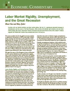
Appendix C Computational experiments All impulse responses shown in Figs. la and lb are expressed as the pecentage deviations from steady state in reaction to a one-standard-deviation positive shock to the technological innovation.

M. Merz / Journal of Monetary Economics 36 (1995) 269-300 Employment N 0.0018 0.0014 0,0010 0,0006 \

0.0002 -0.0002 0

20

40

60

80

100

120

80

100

120

80

100

120

Unemployment U 0.006 f"

-0.002 -0.010 -0.018 -0,026 20

40

60

Vacancies V 0.026 0,022 0.018 0.014 0.010 0.006 0.002 20

40

60

Search intensity S 0.026 0.022 j~ 0.018 0.014 0.010 _~l \ \ 0.006 -0.002

" 20

40

~

60

-

~ 80

--100

120

Fig. la. Impulse responses with variable search intensity S.

295

296

M. Merz / Journal o f Monetary Economics 36 (1995) 269-300 Labor productivity P 0.0036 0.0028 0.0020 0.0012 0.O004 0

20

40

60

80

100

120

Real wage w 0.0024 0.0020 0.0016 0.0012 0.0008 0.0004 0

20

40

60

80

100

120

100

120

100

120

Labor's share LS 0.0002

-0.0006

-0.0014

-0.0022 20

40

60

80

Output Y 0.0045 0.0035 0.0025 0.0015 0.0005 0

20

40

60

80

Fig. la (continued)

M. Merz / Journal of Monetary Economics 36 (1995) 269-300 Employment N 0.0014 0.0010 0.0006

\ \,

0.0002

\,

\•

-0.0002 20

40

60

80

100

120

Unemployment U 0.004 0.000

J

/" /

-0.004

/

-0.008 -0.012 -0.016 -0.020

20

40

60

80

100

120

80

100

120

Vacancies V 0.035 0.030 0.025 0.020 0.015 0.010 0.005 0.000 0

20

40

60

Search intensity S 3.5 Q X

3.0 2.5 2.0 1.5 1.0 0.5 0.0 -0.5

0

20

40

60

80

100

120

Fig. lb. Impulse responses with fixed search intensity S.

297

298

M. Merz / Journal o f Monetary Economics 36 (1995) 269-300 Labor productivity P 0.0036 0.0028 0.0020 0.0012

0.0004 0

20

40

60

80

100

120

100

120

80

1O0

120

80

100

120

Real wage w 0.0024 0.0020 0.0016 0.0012 0.0008 0.0004 0

20

40

60

80

Labor's share LS 0.0002 m

-0.0006

-0.0014

-0.0022 20

40

60 Output Y

0.0045 0.0035 0.0025 0.0015 0.0005 0

20

40

60

Fig. lb (continued)

M. Merz / Journal of Monetary Economics 36 (1995) 269-300

299

References Altonji, J.G., 1982, The intertemporal substitution model of labor market fluctuations: An empirical analysis, Review of Economic Studies 49, 783-825. Altonji, J.G., 1986, Intertemporal substitution in labour supply: Evidence from micro data, Journal of Political Economy 94, S176-$215. Andolfatto, D., 1993, Business cycles and labor market search, Unpublished manuscript (University of Western Ontario, London). Ashenfelter, O., 1984, Macroeconomic analyses and microeconomic analyses of labor supply, in: K. Brunner and A.H. Meltzer, eds., Essays on macroeconomic implications of financial and labor markets and political processes, Carnegie-Rochester Conference Series on Public Policy 21, 117 155. Blanchard, O.J. and P. Diamond, 1989, The Beveridge curve, Brookings Papers on Economic Activity, 1-60. Blanchard, O.J. and P. Diamond, 1990, The aggregate matching function, in: Peter Diamond, ed., Productivity/growth, unemployment (MIT Press, Cambridge, MA) 159 201. Christiano, L.J., 1987, Why does inventory investment fluctuate so much? Technical appendix, Working paper no. 380 (Federal Reserve Bank of Minneapolis, Minneapolis, MN). Christiano, L.J., 1988, Why does inventory investment fluctuate so much?, Journal of Monetary Economics 21,247 280. Christiano, L.J. and M.S. Eichenbaum, 1992, Current real business cycle theories and aggregate labor market fluctuations, American Economic Review 86, 430-450. Danthine, J.-P. and J.B. Donaldson, 1989, Risk sharing, the minimum wage and the business cycle, Working paper no. 9018 (Universit6 de Lausanne, Lausanne). Hansen, G.D., 1985, Indivisible labor and the business cycle, Journal of Monetary Economics 16, 309-327. Hodrick, R.J. and E.C. Prescott, 1980, Post-war U.S. business cycles: An empirical investigation, Unpublished manuscript (Carnegie-Mellon University, Pittsburgh, PA). Hosios, A.J., 1990, On the efficiency of matching and related models of search and unemployment, Review of Economic Studies 57, 279-298. Jackman, R., R. Layard, and S. Nickel, 1991, Unemployment, macroeconomic performance and the labor market (Oxford University Press, Oxford). King, R.G., C.I. Plosser, and S. Rebelo, 1989, Production, growth and business cycles: Technical appendix, Unpublished manuscript (University of Rochester, Rochester, NY). Kydland, F.E. and E.C Prescott, 1982, Time to build and aggregate fluctuations, Econometrica 50, 1345-1370. Long, J,B. and C. Plosser, 1983, Real business cycles, Journal of Political Economy 91, 39--69. Lucas, R.E., Jr., 1987, Models of business cycles (Basil Blackwell, Oxford). MaCurdy, T.E., 1981, An empirical model of labor supply in a life-cycle setting, Journal of Political Economy 89, 1059-1085. Millard, S.P. and D.T. Mortensen, 1994, The unemployment and welfare effects of labor market policies: A case for hiring subsidy, Unpublished manuscript (Northwestern University, Evanston, IL). Moen, E.R., 1993, A search model with wage announcements, Unpublished manuscript (London School of Economics, London). Mortensen, D.T., 1992, Equilibrio de busqueda y ciclos economicos reales, Cuadernos Economicos 51, 151-172. Mortensen, D.T., 1994, The cyclical behavior of job and worker flows, Journal of Economic Dynamics and Control 18, 1121-1142. Mortensen, D.T. and C. Pissarides, 1993, The cyclical behavior of job creation and job destruction, in: J.C. van Ours, G.A. Pfann, and G. Ridder, eds., Labour demand and equilibrium wage formation (North-Holland, Amsterdam) 201-222.

300

M. Merz / Journal o f Monetary Economics 36 (1995) 269-300

van Ours, J.C. and G. Ridder, 1992, Vacancies and the recruitment of new employees, Journal of Labor Economics 10, 138 155. Phelps, E.S., ed., 1970, Microeconomic foundations of employment and inflation theory (Norton, New York, NY). Pissarides, C.A., 1986, Unemployment and vacancies in Britain, Economic Policy 3, 499-559. Pissarides, C.A., 1988, The search equilibrium approach to fluctuations in employment, American Economic Review, Papers and Proceedings 78, 363-368. Pissarides, C.A., 1990, Equilibrium unemployment theory (Basil Blackwell, Oxford). Prescott, E.C. and R. Mehra, 1980, Recursive competitive equilibrium: The case of homogeneous households, Econometrica 48, 1365-1379. Rogerson, R., 1988, Indivisible labor, lotteries and equilibrium, Journal of Monetary Economics 21, 3-16. Rotemberg, J.J. and M. Woodford, 1991, Oligopolistic pricing and the effects of aggregate demand on economic activity, Unpublished manuscript (MIT, Cambridge, MA; University of Chicago, Chicago, IL). Shouyong, S. and Q. Wen, 1994, Unemployment and the dynamic effects of factor taxation, Unpublished manuscript (Queen's University, Kingston).