Ecology, 83(8), 2002, pp. 2240–2247 q 2002 by the Ecological Society of America
SCALING UP ANIMAL MOVEMENTS IN HETEROGENEOUS LANDSCAPES: THE IMPORTANCE OF BEHAVIOR JUAN MANUEL MORALES1,3
AND
STEPHEN P. ELLNER2,4
1Department
of Zoology, North Carolina State University, Raleigh, North Carolina 27695 USA Biomathematics Program, Department of Statistics, North Carolina State University, Raleigh, North Carolina 27695-8203 USA
2
Abstract. Two major challenges of spatial ecology are understanding the effects of landscape heterogeneity on movement, and translating observations taken at small spatial and temporal scales into expected patterns at greater scales. Using a combination of computer simulations and micro-landscape experiments with Tribolium confusum beetles we found that conventional correlated random walk models with constant parameters severely underestimated spatial spread because organisms changed movement behaviors over time. However, a model incorporating behavioral heterogeneity between individuals, and within individuals over time, was able to account for observed patterns of spread. Our results suggest that the main challenge for scaling up movement patterns resides in the complexities of individual behavior rather than in the spatial structure of the landscape. Key words: animal movement; correlated random walk; diffusion; land-management information; landscape heterogeneity, and movement; model, individual based; population heterogeneity; random walk models; scaling up; spatial ecology; Tribolium confusum.
INTRODUCTION Movement of organisms within heterogeneous landscapes is a key process (Kareiva 1990, Wiens et al. 1993, Turchin 1998) influencing metapopulation dynamics, the coexistence of competitors, community structure, disease ecology, and biological invasions (Tilman 1994, Keeling and Grenfell 1997, Shigesada and Kawasaki 1997, Tilman and Kareiva 1997, Hanski 1998). Practical limitations in measuring and analyzing movement often result in descriptions based on data collected at small spatial scales and/or in phenomenological models of dispersal (Kareiva and Andreasen 1988). A mechanistic way to scale up movement in heterogeneous landscapes is both theoretically appealing and critically needed to assess the potential effects of habitat loss or modifications for landscape management and conservation. Random walk models and their diffusion approximations have been the most successful and widely used mechanistic models to describe movement at the scale of data collection, but they may give unrealistic predictions when extrapolated to other scales (Turchin 1996). At larger scales, movement behavior can change as individuals encounter different habitats, and as they engage in different activities (Firle et al. 1998). FurManuscript received 5 October 2001; accepted 11 December 2001. 3 Present address: Department of Ecology and Evolutionary Biology, University of Connecticut, 75 North Eagleville Road, Storrs, Connecticut 06269 USA. E-mail:
[email protected] 4 Present address: Department of Ecology and Evolutionary Biology, Corson Hall, Cornell University, Ithaca, New York 14853-2701 USA.
thermore, many organisms are reluctant to cross certain habitat boundaries, and, consequently, their movement patterns are strongly affected by landscape structure (Stamps et al. 1987, Tischendorf and Wissel 1997, Haddad 1999). We used an experimental model system (EMS; Wiens and Milne 1989, Ims et al. 1993) to examine whether a random walk framework can be used to translate small-scale, within-patch movement data to larger scale spread in heterogeneous landscapes. EMS designs are useful in studies of the effects of landscape heterogeneity on movement since they allow manipulation that would not be feasible in real landscapes. We worked with adult Tribolium confusum beetles (Coleoptera, Tenebrionidae) walking on ‘‘fast’’ and ‘‘slow’’ artificial substrates constructed with paper and masking tape. These substrates were chosen to represent habitat types or land cover types that influenced movement patterns, but presented no attraction for beetles (food, shelter, or conspecifics). We also manipulated edge effects by fixing habitat boundaries with Scotch Magic Tape (3M, Saint Paul, Minnesota, USA), which has a slippery surface and served to lower the probability that a beetle would leave the habitat patch upon reaching an edge (the tape). Tribolium beetles did not evolve to walk over landscapes of paper and tape. However, such experimental model systems provide a useful halfway house between mathematical models and complex realworld landscapes where it would be difficult to relate movement decisions to specific habitat attributes. Previous studies using EMS to study movement have focused mainly on how microlandscape heterogeneity affects movement statistics such as movement rate, path length, and tortuosity (Crist et al. 1992, Wiens et
2240
SCALING UP ANIMAL MOVEMENTS
August 2002
2241
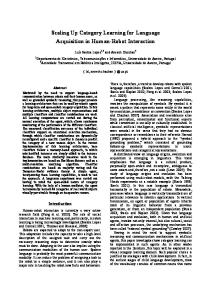
FIG. 1. Schematic representation of the heterogeneous microlandscapes. Panel (a) depicts a heterogeneous microlandscape with 20% of patches of ‘‘slow habitat’’ (shaded) distributed at random. The zoomed area shows the arrangement of squares of masking tape used to alter beetle movement in the slow habitat. Panel (b) is the same as (a), but with boundaries (‘‘edges’’) between different habitats.
al. 1997, McIntyre and Wiens 1999a, b, With et al. 1999). Inspired by percolation theory, some authors simulated movement in EMS as random walks over square lattices of accessible and inaccessible cells (e.g., Johnson et al. 1992, With et al. 1999). Here we used our EMS to parameterize a set of more realistic movement models from small-scale movement observations, and to test their ability to predict movement over larger spatial and temporal scales. We show that a conventional correlated random walk model with constant parameters severely underestimated the rate of spatial spread because organisms changed movement behaviors over time. However, a model incorporating behavioral heterogeneity between individuals, and within individuals over time, was able to account for the observed patterns of spread. EXPERIMENTS
Within-patch movement We constructed 25 3 25 cm patches of two different substrates. The ‘‘fast habitat’’ consisted of plain paper, and the ‘‘slow habitat’’ was paper where 2 3 2 cm squares of masking tape were centered at 5-cm intervals along staggered rows separated by 2.5 cm (see zoomed patches in Fig. 1). The boundaries of these patches were fixed with Magic Tape. For each habitat type, we quantified the distributions of movement components (step length and turning angle), by videotaping the movement of 50 beetles. Individuals were released one at a time and their movement recorded for several minutes. Beetles moving in the slow habitat were often faced with obstacles (pieces of tape, sticky side down), and forced to slow down and to make bigger turns. All experiments were conducted at room temperature and room illumination after sunset. Beetles almost never stopped moving during the course of these trials. Their position every 4 s was obtained as x and y coordinates using software developed by N. F. Hughes and L. H.
Kelly (Hughes and Kelly 1996). The distance between two consecutive fixes defined a step length, and the angular difference in the compass direction of two consecutive steps defined a turning angle. The temporal scale of fixes was chosen after inspection of the movement paths, in order to reflect the time scale of beetle movement behavior (Turchin 1998). We also observed whether beetles crossed from one habitat to the other after bumping into the Magic Tape, and calculated the probability of crossing habitat boundaries as the number of boundary crosses divided by the number of boundary encounters (44/710 5 0.062). We recorded 101 paths in fast habitat (647 steps and 543 turning angles), and 76 paths in slow habitat (785 steps and 691 turning angles). Beetles moving in fast patches showed greater step lengths (4.92 6 1.58 cm [mean 6 1 SD]), and smaller turning angles (cosine 5 0.60 6 0.57 [mean 6 1 SD]) compared to slow patches (step length 5 3.70 6 1.53 cm; cosine 5 0.40 6 0.65). There was no bias in turning angle in any of the patch types (i.e., mean sine not different from zero: fast patches, sine 5 20.004, t 5 0.18; slow patches, sine 5 20.036, t 5 1.46).
Microlandscape experiment 1 We established three different mosaic microlandscapes consisting of a 16 3 16 grid of habitat patches (4 3 4 m): (1) homogeneous (all fast habitat); (2) 20% of slow habitat without edges, (3) 20% of slow habitat with edges. The location of slow-habitat patches in the heterogeneous microlandscapes [(2) and (3)] was chosen at random (Fig. 1). We chose a proportion of 20% of slow habitat based on Wiens et al.’s (1997) experiment with darkling beetles, where they found strong differences between movement pattern in homogeneous habitats (sand) and microlandscapes with 20% grass coverage, but little difference between 20% and 80% grass coverage. In our experiment, microland-
2242
JUAN MANUEL MORALES AND STEPHEN P. ELLNER
scapes were constructed by seaming strips of standard brown wrapping paper (92 cm wide). Edge effects were created by pasting strips of Magic Tape at the boundaries between slow and fast habitat. Beetles were picked at random from the rearing medium, where the sex ratio was 1:1, and checked for general condition (size, complete appendages, etc.). They were left a few minutes in the center of the landscape under a plastic cup before being released. Beetles moved readily after release and very rarely stopped during the course of the experiments. Each individual was released only once in the experimental arena to avoid learning or other factors that could complicate the outcome of the experiments. All experiments were conducted at room temperature and room illumination after sunset. Beetles were followed for 20 min after release, or until they left the experimental arena, whichever occurred first. The size of the microlandscapes prevented the use of video to track beetle position. Instead, we used a predefined grid where we mapped individual spatial coordinates at fixed time intervals. The microlandscape area was subdivided by lines drawn with pencil, delimiting numbered cells of 25 3 25 cm which were further divided into 5 3 5 cm squares. By visually judging which corner of a 5 3 5 cm square was closest to an individual, we were able to record beetle spatial coordinates with a resolution of 2.5 cm. A total of 50 beetles were released one at a time in the center of each microlandscape, and their position was recorded every 40 s for the homogeneous landscape, and every 20 s for the other landscapes.
Ecology, Vol. 83, No. 8
lated random walk (CRW; Kareiva and Shigesada 1983). The spatial position of an organism was represented by continuous x and y coordinates projected onto landscape maps consisting of fast- and slow-habitat patches. At every iteration of the model, individuals chose a step length and a turning angle according to the empirically observed distribution of these variables for the patch type in which they were located. Hence, the temporal scale of the model iteration was 4 s. Edge effects were incorporated as fixed probabilities of crossing a boundary between different patch types. As expected (Wiens et al. 1997), beetle spread in the landscape experiments was fastest in the homogeneous landscape and slowest in the landscape composed of 20% slow habitat with edges. However, in all three landscapes beetles spread considerably faster than predicted by the CRW simulations. The CRW simulations predicted reasonably well the rate of spread soon after release, but consistently underpredicted large-scale spread (Fig. 2a–c). For the second homogeneous landscape (microlandscape experiment 2), again, our CRW simulation model fit well the increase in mean squared displacement (MSD, average squared Euclidean distance from the point of release) over the first 100 s after release, but observed MSD then began to increase quadratically (Fig. 2d). Beetles in the experimental landscapes showed mean squared displacement growing more rapidly than linearly with time, suggesting that a different movement model would be more appropriate.
Analysis of movement paths Microlandscape experiment 2 In order to identify possible causes of the failure of our simulation models to predict larger spatial-scale spread (see results in Fig. 2, below), we conducted another experiment in a new homogeneous landscape. We ran 60 beetles and retained for analysis the movement data of 45 individuals who remained in the landscape for at least 400 s. During these trials, we also collected fine-scale movement data at the area of release by videotaping a subset of 25 beetles moving in an area of 4 3 3 cells in the center of the landscape. In this way, we recorded long movement paths necessary to distinguish between oriented and nonoriented movement (Marsh and Jones 1988). We also calculated coarse-scale steps and turning angles using observed beetle positions at 20-s intervals. Note that these steps correspond to five iterations of our simulation model, and that they represent the outcome of several fine-scale movement decisions. MOVEMENT MODELS
Correlated random walk Data from the within-patch movement experiment were used to parameterize a spatially explicit, individual-based model that simulated movement as a corre-
To explore possible ways of modifying our simulation models, we performed a series of analyses on the movement paths from the microlandscape experiment 2. The first alternative considered was biased random walk (BRW). The CRW model assumes that the direction of a step is only related to the direction of the previous one. Therefore, the compass direction of steps that are separated by enough time will be independent, yielding MSD that grows linearly over long time scales. In contrast, the turning angles in a BRW model are chosen relative to a fixed compass direction. This results in MSD growing quadratically with time. However, a CRW with little variance in turning angles and/ or high-order autocorrelation in turns can also produce a quadratic increase in MSD for a considerable time. To distinguish between the BRW and CRW models, we used Marsh and Jones’s (1988) D statistic: D5
[1O cos u 2 1 1O sin u 2 ] 1 2 O cos v 2 1 1O sin v 2 ]. (n 2 1) [1 2
1 n2
2
j
j
2
2
j
2
j
(1)
Here uj are the direction angles (i.e., the compass direction measured in radians) of the n observed moves, and the vj are the turning angles between successive
August 2002
SCALING UP ANIMAL MOVEMENTS
2243
FIG. 2. Spread of Tribolium confusum in the experimental microlandscapes: (a) homogeneous microlandscape composed entirely of ‘‘fast’’ habitat; (b) 20% of the microlandscape is ‘‘slow’’ habitat; (c) same as (b) but with habitat boundaries; (d) second homogeneous, all fast habitat, microlandscape. Error bars are 61 SE for the mean squared displacement (MSD) over individual beetles, and solid lines are 95th-percentile intervals from the distribution of MSD obtained by 1000 replicates of the simulation of 50 individual movement paths. The leveling off of MSD in (a) and (b) is due to the fastest moving beetles leaving the experimental area quickly.
moves. The expectation of D is positive for BRW, and negative for CRW. We compared the value of D for observed movement paths with the theoretical distribution of D for animals moving as BRW or CRW. The theoretical distribution of D depends on the number of individuals tracked and number of observed moves for each individual, and were obtained by Marsh and Jones through extensive simulation. The ideal resolution for conducting this test was 4 s, corresponding to the scale of beetle behavior and model iteration. However data at that resolution were only available for the area near the release point in the microlandscapes, and movement paths spanning the entire arena were observed only at the coarser resolution (20 s). We therefore conducted the Marsh and Jones test in three ways: (1) at 4-s resolution, to determine whether a BRW model would be better from the outset, (2) for entire movement paths at 20-s resolution, and (3) for the final 10 steps at 20s resolution, to explore the possibility of a switch to BRW over the course of the experiments. The second alternative that we explored was that beetles change their movement behavior over time. We tested this hypothesis (against the alternative of no
change in behavior) with a randomization test, by randomly permuting the time order of observed step lengths and turning angles within individual beetles. Test statistics were the slope and intercept from linear regression of step length and of angular variance of turning angles on time, and P values were calculated after 5000 randomizations. To test whether only some beetles changed behavior, we looked for individual beetles whose maximum displacement from the release point exceeded the 95th percentile for simulated beetles moving as a CRW with constant movement parameters fitted to our experimental data. Percentiles of maximum displacement for an individual under the CRW model were calculated by simulating 5000 individuals moving during 400 s. Although quadratic increase in MSD is typical of BRW, the Marsh and Jones (1988) test determined that small-scale movements near the release point (4-s resolution) were consistent with CRW but not with BRW, while comparison of BRW and CRW models for largescale movement observations was inconclusive (Table 1). Rather, over time the beetles exhibited a significant increase in the length of coarse-scale (20-s) movement
2244
JUAN MANUEL MORALES AND STEPHEN P. ELLNER
Ecology, Vol. 83, No. 8
TABLE 1. Marsh and Jones (1988) test for consistency of movement data with biased random walk (BRW) and correlated random walk (CRW) models. Data scope†
Observed D
N
BRW
Small scale‡ (4 sec) Large scale§ (20 sec) Final 10 moves (20 sec)
20.0638 0.006 0.02812
24 45 45
(20.0245, 0.0244) (20.0236, 0.0636) (20.0257, 0.0627)
CRW (20.1159, 20.0261) (20.0542, 0.0342) (20.0483, 0.0283)
Notes: Delta (D) is a statistic computed from movement observations (Eq. 1). We applied it to the data from microlandscape experiment 2. The ‘‘95% interval’’ for each model is the range having a 95% chance of containing the value of D, given the number of observations N. Values of D outside the interval imply that the model can be rejected at the 5% significance level. † Scale of resolution is in parentheses. ‡ First 190 6 24 sec (mean 6 1 SE) after release. § Entire movement paths.
steps and a decreased variance in coarse-scale turning angles (step length: slope 5 0.0101, P , 0.01; intercept 5 10.427, P , 0.01; angular variance of turning angles: slope 5 20.0008, P , 0.01; intercept 5 0.8439, P , 0.01). Together, these results suggest a CRW model with changing parameters. According to the linear-regression equations, over the first 10 min following release there was a 58% increase (on average) in coarsescale step length, and a 57% decrease in the angular variance of turning angles. However considering each beetle individually, significant evidence (P , 0.05) for a departure from CRW with constant movement parameters was found in only 15 of 45 beetles.
tribution, which has the advantage of being easily implemented for simulation, and allows the mean angle and angular variance to be specified independently. In the BRW section of the switching model, the mean angle for the distribution was set equal to the compass direction of the last CRW step, and with a new, timeinvariant, turning-angle variance (vb). The time for behavioral switch (148 s) was determined by a nonlinear least-squares procedure on the following regression model:
Modified random walk models
where MSD is observed mean squared displacement over time (t), and d is the time of switch from linear to quadratic response. Step length in both models was increased as
Based on the analysis of movement paths, we considered two possible modifications of our original model: an ‘‘acclimating’’ model that assumes that the variance of turning angles decreases exponentially over time, and a ‘‘switching’’ model in which beetles switch from a CRW model to a BRW model at a fixed time after release. Other functions could be used to model the decrease in turning-angle variance in the acclimating model, but within the resolution of our data on turning-angle variance (Fig. 3) the exponential model provides an adequate fit with only one parameter. Both of these models were simulated by sampling from the observed distribution of fine-scale movement steps, and incorporating the observed increase in step length over time. We then asked whether any combination of parameter values describing the fine-scale movement rules would fit the observed trends over time in largescale turning-angle variance, large-scale step length, and MSD. Simulations were done in two ways: (1) assuming that all beetles change behavior over time, and (2) assuming that only 15 beetles change behavior. Turning-angle variance in the acclimating model changed as
v(n) 5 v0exp(2dn)
(2)
where v is a measure of angular variance, v0 is initial variance, n is the simulation iteration number, and d is a parameter controlling the rate of reduction in angular variance. We used the Firle et al. (1998) angular dis-
MSD(t) 5
5a
a 1 bt 1 bt 1 c (t 2 d )
t#d 2
s(n) 5 (1 1 w n)b(n)
t.d
(3)
(4)
where s(n) is the length of the nth movement step, b(n) is step length obtained by bootstrap sampling from the data (i.e., chosen at random with replacement), and w is a parameter that regulates the rate at which mean step length increases over time. For homogeneous populations (i.e., all individuals behaving in the same way), both modified random walk models were able to fit the observed patterns of changes in coarse-scale step length and turning-angle variance, but they were unable to fit the observed MSD (Fig. 3). The acclimating model underpredicted MSD, and the switching model overpredicted MSD. However when only a fraction of the simulated individuals changed behavior, the acclimating model was able to fit the three movement statistics without an increase in fine-scale step lengths (w 5 0); the increase in coarse-scale step length was entirely due to the reduction in turningangle variance for the fine-scale steps. As a further test of the acclimating model we attempted to fit the coarse-scale data on movements in heterogeneous microlandscapes. For this comparison we extended the acclimating-model simulations to include the observed boundary-crossing probabilities, and to have different step length and turning-angle var-
SCALING UP ANIMAL MOVEMENTS
August 2002
2245
FIG. 3. Modified random walk models fit to beetle movement in microlandscape experiment 2 (homogeneous landscape, all ‘‘fast’’ habitat). Squares are observed values, and error bars are 61 SE. Dashed lines are 95th-percentile intervals for the homogeneous population models, and solid lines are 95th-percentile intervals for heterogeneous population models (15 out of 45 individuals changing movement behavior). Percentile intervals for all the models were calculated from 1000 simulations of 45 individual movement paths. MSD 5 mean squared displacement (distance from beetle point of release). The three lefthand panels correspond to the ‘‘acclimating’’ model where beetles reduce turning-angle variance exponentially with time at rate d (Eq. 2); d 5 0.015 for the homogeneous population model and d 5 0.05 for the heterogeneous population model. For both models the initial turning-angle variance (v0 in Eq. 2) is 0.5, and there is no increase in fine-scale step length (parameter w 5 0 in Eq. 4). The three right-hand panels correspond to the ‘‘switching’’ model where beetles switch from correlated random walk (CRW) to biased random walk (BRW) at a fixed point in time. The turning-angle variance for the biased part of the walk (vb) is 0.95 for the homogeneous population model and 0.5 for the heterogeneous population model. The rate of increase in fine-scale step length parameter w is 0.175 for both models.
iance for the two patch types. With these extensions, the acclimating model was also able to fit the movement statistics observed in the heterogeneous landscapes (Fig. 4). DISCUSSION Our results illustrate the difficulties of extrapolating movement observations to larger temporal and spatial scales. Even within the relatively short time scale of our microlandscape experiments, moving organisms violated the assumption of constant movement behavior. It is well established that the physiological state of individuals can alter movement behavior (Bell 1991).
Food-deprived Drosophila melanogaster increase the time spent in intensive-search mode upon encounter of food as their time of starvation increases (Bell et al. 1985). Gut fullness has been used in a series of advection diffusion models for area-restricted search of predators (Kareiva and Odell 1987, Gru¨ nbaum 1998). For the experimental system used here, it is unlikely that changes in turning-angle distributions resulted from beetles getting hungry. Prior to their release, beetles were immersed in food, and they only stayed in the experimental landscapes for a maximum of 15 min. The experimental microlandscape was likely to seem hostile for the beetles. There was no food, shelter, or
2246
JUAN MANUEL MORALES AND STEPHEN P. ELLNER
Ecology, Vol. 83, No. 8
FIG. 4. Acclimating model fit to beetle movement in microlandscape experiment 1, with 20% ‘‘slow habitat’’ patches. Solid lines are 95th-percentile intervals for the models calculated from 1000 simulations of 45 individual movement paths. The three left-hand panels present results with no edge effects; for the three right-hand panels, edge effects were added (probability of boundary cross 5 0.06). In the models, 15 out of 45 individuals changed behavior. Initial turning-angle variance (v0 in Eq. 2) equals 0.5 for fast habitat and 0.6 for slow habitat. The rate of reduction in turning-angle variance (d) for beetles that changed movement behavior is 0.05 for all habitats.
conspecifics. It is reasonable to think that individuals were modifying their movement behavior to escape from the experimental arena. Convoluted paths result in a thorough exploration of an area, but paths with a strong linear component (but not perfectly straight) are more effective to locate resources that are widely spaced (Zollner and Lima 1999). Within the same type of patches, and depending on their physiological state and/or time since the beginning of movement, organisms could alternate between a thorough exploration (with high variance in turning angles) and escape from an area that is not suitable for them. The failure of the correlated random walk (CRW) model to describe movement at larger scales was caused by changes in individual movement behavior rather than by effects of landscape heterogeneity or habitat boundaries. In other words, our results suggests that the main challenge of scaling up movement resides
in the complexities of individual behavior rather than in the spatial structure of the landscape, which could be relatively easily mapped and incorporated into computer simulations. This claim is supported by the good fit of the CRW model during the first 100 s of the microlandscape experiments (Fig. 2c and d). Moreover, spatial heterogeneity and boundary reactions were easily incorporated in the acclimating model, allowing us to fit the experimental observations (Fig. 4). Our results also illustrate the value of comparing more than one aspect of model output to observations. Both acclimating and switching models could fit the observed mean squared displacement (MSD) under certain parameter combinations (results not shown), but only the acclimating model was able to fit the changes in step length, turning-angle variance, and MSD. Conservation and land-use planning require us to understand the connection between landscape pattern
SCALING UP ANIMAL MOVEMENTS
August 2002
and the dynamics of populations on the landscape, and theory suggests that we must understand movement and dispersal in order to do so (Kareiva and Wennergren 1995). Although our experimental system incorporated some aspects of landscape heterogeneity, it is far simpler than any real landscape, and was sufficiently different from the study organism’s natural habitat that complex behavioral responses to habitat properties might not be expected. Nonetheless we found that scaling up from small-scale measurements to predict the rate of population spread across the landscape was not possible without taking into account behavioral variability between individuals and within a single individual over time. Although simple random walk models for homogeneous populations with constant parameters have provided valuable insights into the spatial dynamics of populations, accurate predictions at the landscape scale will require models that can accommodate the complexities of individual behavior and behavioral dynamics (Lima and Zollner 1996, Roitberg and Mangel 1997). ACKNOWLEDGMENTS We thank Martha Groom, Jim Gilliam, Peter Turchin, Jeremy Lichstein, two anonymous referees, and the editor (Bill Gurney) for useful comments. Andy Amacher, Todd Preuninger, Roxana Arago´n, and Toma´s Carlo helped with the experiments. Pete Rand kindly provided the digitizing equipment. This work was supported by a Fulbright fellowship to J. M. Morales. LITERATURE CITED Bell, W. J. 1991. Searching behavior: the behavioral ecology of finding resources. Chapman and Hall, London, UK. Bell, W. J., C. Tortorici, R. J. Roggero, L. R. Kipp, and T. R. Tobin. 1985. Sucrose-stimulated behaviour of Drosophila melanogaster in a uniform habitat: modulation by period of deprivation. Animal Behaviour 33:436–448. Crist, T. O., D. S. Guertin, J. A. Wiens, and B. T. Milne. 1992. Animal movement in heterogeneous landscapes: an experiment with Eleodes beetles in shortgrass prairie. Functional Ecology 6:536–544. Firle, S., R. Bommarco, B. Ekbom, and M. Natielo. 1998. The influence of movement and resting behavior on the range of three carabid beetles. Ecology 79:2113–2122. Gru¨nbaum, D. 1998. Using spatially explicit models to characterize foraging performance in heterogeneous landscapes. American Naturalist 151:97–115. Haddad, N. M. 1999. Corridor use predicted from behaviors at habitat boundaries. American Naturalist 153:215–227. Hanski, I. 1998. Metapopulation dynamics. Nature 396:41– 49. Hughes, N. F., and L. H. Kelly. 1996. New techniques for 3D video tracking of fish swimming movements in still or flowing water. Canadian Journal of Fisheries and Aquatic Sciences 53:2476–2483. Ims, R. A., J. Rolstad, and P. Wegge. 1993. Predicting space use responses to habitat fragmentation: Can voles Microtus oeconomus serve as an experimental model system (EMS) for capercaillie grouse Tetrao urogallus in boreal forest? Biological Conservation 63:261–268. Johnson, A. R., B. T. Miline, and J. A. Wiens. 1992. Diffusion in fractal landscapes: simulations and experimental studies of tenebrionid beetle movements. Ecology 73:1968–1983. Kareiva, P. M. 1990. Population dynamics in spatially complex envionments: theory and data. Philosophical Trans-
2247
actions of the Royal Society of London Series B 330:175– 190. Kareiva, P., and M. Andreasen. 1988. Spatial aspects of species interactions: the wedding of models and experiments. Pages 35–50 in A. Hastings, editor. Community ecology. Springer Verlag, New York, New York, USA. Kareiva, P., and G. Odell. 1987. Swarms of predators exhibit ‘‘preytaxis’’ if individual predators use area-restricted search. American Naturalist 130:233–270. Kareiva, P. M., and N. Shigesada. 1983. Analyzing insect movement as a correlated random walk. Oecologia 56:234– 238. Kareiva, P. M., and U. Wennergren. 1995. Connecting landscape patterns to ecosystem and population processes. Nature 373:299–302. Keeling, M. J., and B. T. Grenfell. 1997. Disease extinction and community size: modeling the persistence of measles. Science 275:65–67. Lima, S. L., and P. A. Zollner. 1996. Towards a behavioral ecology of ecological landscapes. Trends in Ecology and Evolution 11:131–135. Marsh, L. M., and R. E. Jones. 1988. The form and consequences of random walk movement models. Journal of Theoretical Biology 133:113–131. McIntyre, N. E., and J. A. Wiens. 1999a. How does habitat patch size affect animal movement? An experiment with darkling beetles. Ecology 80:2261–2270. McIntyre, N. E., and J. A. Wiens. 1999b. Interactions between habitat abundance and configuration: experimental validation of some predictions from percolation theory. Oikos 86:129–137. Roitberg, B. D., and M. Mangel. 1997. Individuals on the landscape: behavior can mitigate lanscape differences among habitats. Oikos 80:234–240. Shigesada, N., and K. Kawasaki. 1997. Biological invasions: theory and practice. Oxford University Press, New York, New York, USA. Stamps, J. A., M. Buechner, and V. V. Krishnan. 1987. The effects of edge permeability and habitat geometry on emigration from patches of habitat. American Naturalist 129: 533–552. Tilman, D. 1994. Competition and biodiversity in spatially structured habitats. Ecology 75:2–16. Tilman, D., and P. Kareiva, editors. 1997. Spatial ecology: the role of space in population dynamics and interspecific interactions. Princeton University Press, Princeton, New Jersey, USA. Tischendorf, L., and C. Wissel. 1997. Corridors as conduits for small animals: attainable distances depending on movement pattern, boundary reaction and corridor width. Oikos 79:603–611. Turchin, P. 1996. Fractal analyses of animal movements: a critique. Ecology 77:2086–2090. Turchin, P. 1998. Quantitative analysis of movement: measuring and modeling population redistribution in animals and plants. Sinauer Associates, Sunderland, Massachusetts, USA. Wiens, J. A., and B. T. Milne. 1989. Scaling of ‘‘landscapes’’ in landscape ecology, or, landscape ecology from a beetle’s perspective. Landscape Ecology 3:87–96. Wiens, J. A., R. L. Schooley, and R. D. J. Weeks. 1997. Patchy landscapes and animal movements: Do beetles percolate? Oikos 78:257–264. Wiens, J. A., N. C. Stenseth, B. Van Horne, and R. A. Ims. 1993. Ecological mechanisms and landscape ecology. Oikos 66:369–380. With, K. A., S. J. Cadaret, and C. Davis. 1999. Movement responses to patch structure in experimental fractal landscapes. Ecology 80:1340–1353. Zollner, P. A., and S. L. Lima. 1999. Search strategies for landscape-level interpatch movements. Ecology 80:1019– 1030.