Scalable Fine-Grained Behavioral Clustering of HTTP-Based Malware Roberto Perdiscia , Davide Ariub , Giorgio Giacintob a

Department of Computer Science, University of Georgia 415 Boyd Graduate Studies Research Center Athens, GA 30602-7404 b Department of Electric and Electronic Engineering, University of Cagliari Piazza d’Armi, 09123 Cagliari, Italy

Abstract A large number of today’s botnets leverage the HTTP protocol to communicate with their botmasters or perpetrate malicious activities. In this paper, we present a new scalable system for network-level behavioral clustering of HTTP-based malware that aims to efficiently group newly collected malware samples into malware family clusters. The end goal is to obtain malware clusters that can aid the automatic generation of high quality network signatures, which can in turn be used to detect botnet command-and-control (C&C) and other malware-generated communications at the network perimeter. We achieve scalability in our clustering system by simplifying the multistep clustering process proposed in [31], and by leveraging incremental clustering algorithms that run efficiently on very large datasets. At the same time, we show that scalability is achieved while retaining a good trade-off between detection rate and false positives for the signatures derived from the obtained malware clusters. We implemented a proof-of-concept version of our new scalable malware clustering system and performed experiments with about 65,000 distinct malware samples. Results from our evaluation confirm the effectiveness of the proposed system and show that, compared to [31], our approach can reduce processing times from several hours to a few minutes, and scales well to large datasets containing tens of thousands of distinct malware samples. Email addresses: [email protected] (Roberto Perdisci), [email protected] (Davide Ariu), [email protected] (Giorgio Giacinto)

Preprint submitted to Elsevier Computer Networks

August 15, 2012

Keywords: Malware Clustering, Signature Generation, Network Intrusion Detection 1. Introduction Traditional signature-based anti-virus (AV) tools are mainly based on a static analysis of the code of malicious software (a.k.a. malware), and malware signatures are usually represented by a fixed set of byte sequences in malware executable files [13]. To make AV detection harder, malware writers commonly employ executable packing [16] and other automatic code obfuscation techniques to generate large numbers of polymorphic variants of the same malware [35] that appear syntactically different from each other while remaining semantically similar, so that when executed they perform similar malicious activities. As a consequence, AV companies have a hard time keeping their signature databases up to date, and their AV scanners often suffer from a high rate of false negatives [28]. Therefore, we need new ways to detect malware-compromised machines within a network. Behavioral malware clustering aims at grouping malware variants according to similarities in their malicious behavior. This process is particularly useful because once a number of different variants of the same malware have been identified and grouped together, it is easier to write generic behavioral signatures, as opposed to traditional AV signatures, that may be used to detect future malware variants with low false positives and false negatives. To the best of our knowledge, the behavioral-based systems for clustering and classification of malware proposed so far are heavily based on an analysis of system call traces and system events (e.g., registry modifications, files dropped on disk, etc.) [7, 32, 8, 20], and only limited information from the network traces is used. As a consequence, clustering algorithms such as [7, 8] may generate clusters that are useful when the objective is to extract systemlevel behavioral signatures, but may not perform as well when the goal is to generate network-level behavioral signatures, as shown in [31]. Many of today’s botnets, and many other types of malware, leverage HTTP-based network communications for command-and-control (C&C) purposes or to perpetrate malicious activities. For example, according to [21] the majority of spam botnets use HTTP to communicate with their command and control (C&C) server. Also, [31] found that about 75% of malware samples that exhibit network activities produce HTTP traffic.

2

The motivations for using the HTTP protocol are multiple. Developing a web-based C&C application is typically easier than implementing customized C&C communication protocols (e.g., peer-to-peer protocols), and there is evidence that web-based “reusable” kits (or platforms) for botnet C&C are available for sale on the Internet [12]. Furthermore, many networks (e.g., enterprise and government networks) implement aggressive egress-filtering rules that block unwanted traffic. However, HTTP traffic is allowed in most networks, including networks that implement strict filtering policies, to enable web browsing. This makes it possible for botnet C&C traffic to blend in with legitimate HTTP traffic and reach the botmaster. Therefore, in this paper we focus on behavioral clustering of HTTP-based malware, and we aim to obtain malware clusters that aid in automatically generating network-level behavioral signatures, which can be used to detect malware-generated communications, including botnet C&C traffic, at the network perimeter. Network-level signatures have some attractive properties, compared to system-level signatures. For example, enforcing system-level behavioral signatures often requires the use of virtualized environments and expensive dynamic process analysis [38]. On the other hand, network-level signatures are often easier to deploy, and are able to monitor a large number of machines without introducing any overhead at the end hosts. Although some work has been done towards enabling efficient malware detection using system-level behavioral signatures [22], the proposed technique is limited to malware that does not compromise the operating system’s kernel. Also, in [22] the authors do not apply any behavioral clustering, and the system-level signatures they extract are often too specific, as demonstrated by their relatively low detection rate for certain malware families. Therefore, we believe that a malware detection approach based on network-level behavioral signatures can be a valuable complement to traditional AVs and system-level behavioral signatures, and can play an important role in a comprehensive defense-in-depth strategy against malware. In this paper, we build on previous work by one of the authors [31] and propose a new scalable network-level behavioral malware clustering system that aims at efficiently clustering malware samples according to structural similarities in their HTTP traffic, and to to provide quality input to algorithms that automatically generate network signatures. Namely, after clustering is completed, the HTTP traffic generated by malware samples in the same cluster is processed by an automatic signature generation tool, in order to extract network signatures that model the HTTP behavior of all the mal3

ware variants in a cluster. An Intrusion Detection System (IDS) located at the edge of a network can in turn deploy such network signatures to detect malware-related outbound HTTP requests. The main contribution of this work is scalability, which we achieve by simplifying the multi-step clustering process proposed in [31] and by leveraging incremental clustering algorithms that run efficiently on very large datasets. At the same time, we show that scalability is achieved while retaining a good trade-off between detection rate and false positives for the signatures derived from the obtained malware clusters. We would like to emphasize that scalability is an important requirement for malware clustering and signature generation systems, because it allows us to cope with the increasingly growing number of new malware samples collected every day on the Internet. We implemented a proof-of-concept version of our new malware clustering system and performed experiments with about 65,000 distinct malware samples. Results from our evaluation confirm the effectiveness of the proposed system, and show that, compared to [31], our new clustering approach can reduce processing times from several hours to a few minutes and scales well to large datasets containing tens of thousands of distinct malware samples. 2. Related Work To cope with malware polymorphism, researchers have proposed a number of solutions aimed at enabling the detection of new malware variants based on a set of known malware samples. In [32, 33], Rieck et al. proposed a learning system for analyzing and classifying unknown malware samples based on their system behavior, and in [11], Christodorescu et al. proposed an automatic technique for mining malicious behavior that is present in malware samples but not in benign executables. The extracted behavioral model may than be used as a system-level signature to detect infections by malware from the same family. Behavioral malware clustering has been recently studied in [7, 8, 20, 31]. In particular, Bayer et al. [8] proposed a scalable malware clustering algorithm based on malware behavior expressed in terms of detailed system events. However, the network information they use is limited to high-level features. As a consequence, [8] may generate clusters that are useful when the objective is to extract system-level behavioral signatures, but may not perform as well when the goal is to generate network-level behavioral signatures, as shown in [31]. 4

Anomaly-based detection of malicious HTTP-traffic has been studied for example in [24, 36, 37, 30, 6]. However, anomaly-based detection systems are usually not able to attributed the detected malicious traffic to a specific threat. By using behavioral clustering and signature generation, not only we detect hosts that generate HTTP-based malware traffic, but we can also identify the malware family with which such hosts have been infected. Several data clustering studies addressed the problem of efficiently clustering large volumes of data [5, 14, 15, 40]. CURE [15] employs a combination of random sampling and partitioning to handle large databases. CURE is robust to outliers and is able to identify clusters having non-spherical shapes and wide variances in size. OPTICS [5] does not produce a clustering of a data set explicitly, but instead supports the user in the task of finding the clustering structure. DBSCAN [14] addresses several of the traditional limitations of clustering algorithms. For example, DBSCAN relies on a densitybased notion of clusters which is designed to discover clusters of arbitrary shape, and requires only one input parameter so that it can be easily tuned by the user. To enable efficient malware clustering, in this paper we use the BIRCH clustering algorithm presented in [40], which we discuss in Section 3.2.1. Another relevant problem in data clustering is that of measuring the validity of clustering results. Several different clustering validity indexes have been proposed in the literature [9, 17, 39]. Both the Dunn’s validity index and the Davies-Bouldin (DB) index [17] are internal indexes that aim to asses the quality of clustering by measuring how compact and well separated the clusters are. Other validity indexes include the silhouette statistic [34], and external indexes such as the Rand statistic, Jaccard coefficient, and the Folks-Mallows index [17]. In this paper we make use of the DB index, and of the graph-based cohesion and separation validity indexes proposed in [31], which we briefly describe in Section 3.3.1 and 3.5, respectively. 3. Scalable HTTP-based Behavioral Clustering Problem Definition. In this paper we follow the problem definition given in [31]. The main objective is to perform behavioral clustering of malware samples by finding structural similarities between the sequences of HTTP requests generated by different malware samples as a consequence of infection. In practice, given a dataset of malware samples M = {m(i) }i=1..N , we execute each sample m(i) in a controlled environment similar to BotLab [21] 5

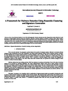
Malware Dataset (HTTP Traces)

Coarse-grained Clustering

Fine-grained Clustering

Signature Generation

(BIRCH)

(Hierarchical Clustering)

(Token Subsequences)

Signature Set

Figure 1: Overview of our new scalable behavioral malware clustering and network signature generation system. for a time T , and we store its HTTP traffic trace H(m(i) ). We then want to partition M into clusters according to a definition of structural similarity among the HTTP traffic traces H(m(i) ), i = 1, .., N , and we aim to do so more efficiently than the clustering system proposed in [31]. 3.1. System Overview In order to attain scalability while maintaining high quality clusters, we adopt the multi-step cluster refinement process shown in Figure 1. • Coarse-grained Clustering: In this phase, malware samples are clustered according to simple statistical features extracted from their malicious HTTP traffic such as the total number of HTTP requests the malware generated, the number of GET and POST requests, the average length of the URLs, etc. Therefore, the similarity between pairs of malware samples reduces to computing the distance between vectors of numbers, and allows us to leverage highly scalable clustering algorithms. This process yields coarse-grained clusters of malware samples that, while they show similar behavior according to our simple statistical features, may belong to different malware families. Therefore, a further step of refinement is necessary to split these coarse-grained results into more accurate clusters. • Fine-grained Clustering: After splitting the collected malware set into relatively large (coarse-grained) clusters, we further split each cluster into smaller groups. To this end, we extract features related to the structure of the HTTP queries generated by the malware samples. This allows us to separate malware that have similar high-level statistical traffic features (thus causing them to fall in the same coarse-grained cluster), but that present different structural characteristics. Measuring the structural similarity between pairs of HTTP traffic traces is relatively expensive. However, since the size of each coarse-grained 6

cluster is much smaller than the total number of samples in the malware dataset, fine-grained clustering can be performed more efficiently than by applying it directly on the entire malware dataset. This clustering step is essentially identical to the fine-grained clustering step used in [31]. • Signature Generation: Afterwards, for each of the obtained fine-grained malware clusters we compute a cluster centroid that “summarizes” the HTTP traffic generated by the malware samples in a cluster. In practice, the centroid of a cluster is represented by a set of network signatures that match (most) malware traffic traces grouped in the cluster. These network signatures are suitable for being deployed at a network IDS to enable the detection of malware-generated traffic (see Section 3.4 for details on the automatic signature generation process). To extract the signature, we use the same automatic signature generation module previously used in [31]. Unlike the three-step clustering process proposed in [31], in this paper we use a much more efficient two-step clustering approach that reduces the overall clustering times from several hours to only a few minutes while retaining a good trade-off between the detection rate and false positives of our malware detection signatures. Compared to [31], we have made the following two key changes. We have replaced the precise hierarchical clustering algorithm used for coarse-grained clustering with an approximate clustering algorithm called BIRCH [40]. As we discuss in Section 3.2.1, BIRCH performs incremental clustering and is suitable for fast clustering over very large datasets. The second important change was to eliminate the meta-clustering step used in [31], which was mainly responsible for merging over-compact clusters that were sometimes obtained due to the use of precise hierarchical clustering in the coarse-grained clustering step. This choice was mainly dictated by the high computational cost of the meta-clustering phase. We noticed that the coarse-grained clustering algorithm used in [31] generated overly compact clusters, few of which could actually be meaningfully refined by the fine-grained clustering step. We then realized that meta-clustering was mainly useful in merging clusters that had been erroneously split during the coarse-grained clustering step. In the end, we found that if we could perform a truly coarse-grained clustering step at the beginning, which would produce relatively large clusters, these clusters could then be meaningfully refined by the fine-grained clustering step without having to go back to merge 7

clusters that we erroneously split during the first clustering phase. As we show in Section 4, our experimental results support our intuition, and show that our new system can achieve the desired scalability while still obtaining high quality malware detection signatures. It is worth noting that the fine-grained clustering step is still performed using precise hierarchical clustering, in a way very similar to [31] (see Section 3.3 for details). The main reason for using precise hierarchical clustering during the fine-grained clustering phase is the fact that to extract good network signatures we need to obtain compact clusters, because otherwise the extracted signatures would risk being over-generic and thus generate a large number of false positives. In addition, hierarchical clustering allows us to perform clustering in arbitrary metric spaces, such as the metric space we define in Section 3.3 to measure the distance between malware samples. 3.2. Coarse-grained Clustering Let M = {m(i) }i=1..N be a set of malware samples, and H(m(i) ) be the HTTP traffic trace obtained by executing a malware m(i) ∈ M for a given time T . We translate each trace H(m(i) ) into a pattern vector v (i) containing the following seven statistical features: the total number of HTTP requests, the number of GET requests, the number of POST requests, the average length of the URLs, average number of parameters in the request, average amount of data sent by POST requests, and the average length of the response. Because the range of different features in the pattern vectors are quite different, we first normalize the dataset, as discussed in Section 4.2.1, and then we partition the set M into coarse-grained clusters by applying the BIRCH clustering algorithm [40] described in Section 3.2.1. 3.2.1. BIRCH Clustering In this Section, we briefly summarize how BIRCH works and outline the main properties that allow for efficient clustering of large datasets. In the interest of space, we refer the reader to [40] for further details. The main goal of BIRCH is to perform approximate clustering of arbitrarily large datasets with a guaranteed (configurable) memory bound and with I/O access costs that grow linearly with the size of the dataset. In other words, the dataset can be scanned only once, and the clustering is performed incrementally. The algorithm trades memory usage for more “coarse” clustering results. In practice, whenever the clustering process approaches the preset memory limit, the clustering algorithm will further “compress” the 8





   



   

 



Figure 2: Overview of BIRCH. Each letter in the CF-tree represents a different sub-cluster. dataset, producing a less fine-grained representation of the data and thus resulting in fewer, larger clusters. BIRCH assumes the objects to be clustered can be represented in a ddimensional vector space (i.e., BIRCH does not support clustering in arbitrary metric spaces). To meet the scalability goals mentioned earlier, BIRCH leverages a data structure called CF-tree, where CF stands for clustering feature. In practice, a CF-tree resembles a B-tree. Each entry of the tree’s nodes is related to a sub-cluster, and each non-leaf entry (i.e., each non-leaf subcluster) represents an agglomeration of a number of child sub-clusters, as depicted in Figure 2. A sub-cluster C = {xi }i=1..n , where the xi are the n single data points that belong to the cluster, is represented as an entry � � of2 the CF-tree by a vector CF (C) = [n, s, ss], where s = i xi and ss = i xi . At the beginning, the CF-tree is empty and data points will be progressively read from the dataset and incrementally added to the tree. When a new data point x is added to a non-empty tree, this new data point will traverse the tree by following the closest child entries. At each given node, if no entry E exists for which dist(x, E) < R, where R is a predefined threshold radius, x will be stored in a new tree entry E� and will effectively form a new sub-cluster. On the other hand, if dist(x, E) < R, x will be merged to the sub-cluster E and CF (E) will be updated. It is worth noting that one could choose different definitions of dist(x, E), as long as the chosen distance function can be efficiently computed by using only E and the information contained in CF (E). Once all data points are entered into the CF-tree, the leaves of the tree provide a representation of the final clusters. 9

If the pre-set memory usage bound is reached, BIRCH automatically increases the value of R and rebuilds the CF-tree by aggregating sub-clusters that are close to each other. In addition, because BIRCH builds the tree incrementally, to mitigate the negative effects of potentially skewed orderings of the data points in the dataset BIRCH includes a number of automatic merging refinements [40] (we have implemented BIRCH in Java, and have made the source code openly available at http://roberto.perdisci.com/ projects/jbirch). 3.3. Fine-grained Clustering In the fine-grained clustering step we consider the structural similarity among sequences of HTTP requests (as opposed to the statistical similarity used for coarse-grained clustering). As in [31], we define the distance between (i) (j) two HTTP requests rk and rh generated by two different malware samples (i) (j) m(i) and m(j) (i.e., rk ∈ H(m(i) ), and rh ∈ H(m(j) )), as (i)

(j)

(i)

(j)

(i)

(j)

dr (rk , rh ) =wm · dm (rk , rh ) + wp · dp (rk , rh ) (i)

(j)

(i)

(j)

+wn · dn (rk , rh ) + wv · dv (rk , rh )

(1)

where the subscripts m, p, n, and v, represent different parts of an HTTP request. Specifically, m represents the request method (e.g., GET, POST, (i) (j) (i) HEADER, etc.), and the distance dm (rk , rh ) is equal to 0 if the requests rk , (j) and rh both use the same method (e.g, both are GET requests), otherwise it is equal to 1. p stands for page, namely the first part of the URL that includes (i) (j) the path and page name, but does not include the parameters. dp (rk , rh ) is equal to the normalized edit distance between the strings related to the (i) (j) path and pages that appear in the two requests rk and rh . n represents the (i) (j) set of parameter names, and dn (rk , rh ) is equal to the Jaccard distance1 between the sets of parameters names in the two requests. v is the set of (i) (j) parameter values, and dv (rk , rh ) is equal to the normalized edit distance between strings obtained by concatenating the parameter values. The factors wx , x ∈ {m, p, n, v} are predefined weights that give more importance to the distance between the requests’ method and page, for example, and less weight to the distance between parameter values. The fine-grained distance between 1

The Jaccard distance between two sets A and B is defined as J(A, B) = 1 −

10

|A∩B| |A∪B|

two samples m(i) and m(j) can then be defined as the average minimum distance between sequences of HTTP requests from the two samples. Given the definition of fine-grained distance between malware samples given above, we apply the single-linkage hierarchical clustering algorithm and the DB cluster validity index (see Section 3.3.1) to split each coarsegrained cluster into fine-grained clusters. 3.3.1. Single-Linkage Hierarchical Clustering As mentioned above, while BIRCH is used for coarse-grained clustering, the fine-grained clustering step relies on precise hierarchical clustering, specifically, single-linkage agglomerative hierarchical clustering. In this section we briefly describe how the hierarchical clustering algorithm works. In order to apply the hierarchical clustering on a set of malware HTTP traces O = {o1 , o2 , ..on }, where oi is the HTTP trace obtained by executing malware sample mi , we first need to define a notion of distance between pairs of traces (we defer the definition of such distance function to Section 3.3). After a distance function dist(oi , oj ) has been defined, we can compute a distance matrix M = {dij }i,j=1..n that consists of the distances dij between each pair of traces (oi , oj ). The hierarchical clustering algorithm takes M as input and produces in output a dendrogram, i.e., a tree-like data structure in which the leaves represent the original traces in O, and the length of the edges represent the distance between clusters [19]. The single-linkage (i) algorithm defines the distance between two clusters Ci = {ok }k=1..ci and (j) (i) (j) Cj = {oh }h=1..cj as δi,j = minl,m {dist(ol , om )}. The obtained dendrogram does not actually define a partitioning of the malware (more specifically their HTTP traces) into clusters, rather it defines “relationships” among malware samples. A partitioning of the set O into clusters can be obtained by cutting the dendrogram at a certain hight h. The leaves that form a connected sub-graph after the cut are considered part of the same cluster [19]. Of course, different values of the height of the cut h may produce different clustering results. Choosing the best clustering involves a cluster validity analysis process to find the value of h that produces the most compact and well separated clusters. In order to automatically find the best value of h, we make use of the Davies-Bouldin (DB) index [17]. The DB index summarizes the intra-cluster

11

dispersion and inter-cluster separation. It can be formally defined as c(h)

DB(h) =

1 � δi + δj max { } c(h) i=1 j=1..c(h),j�=i δi,j

(2)

where δi and δj represent a measure of dispersion for cluster Ci and Cj , respectively, δi,j is the separation (or distance) between two clusters, c(h) is the total number of clusters produced by a dendrogram cut at height h, and DB(h) is the related DB index. The lower the value of the DB index, the more compact and well separated the clusters [17]. Therefore, we can find the best 2 clustering by cutting the dendrogram at height h∗ = arg minh>0 DB(h), where DB(h) is the value of the DB index computed over the clusters obtained by cutting the dendrogram at height h. 3.4. Automatic Signature Generation To perform automatic signature generation, we use the same algorithm described in [31]. We summarize the signature generation process here, and refer the reader to [31] for more details. (i) (i) Let Ci = {mk }k=1..ci be a cluster of malware samples, and Hi = {H(mk )}k=1..ci the related set of HTTP traffic traces obtained by executing each malware sample in Ci . Each signature sj is extracted from a pool pj of HTTP requests selected from the traffic traces in Hi . To create an HTTP request pool, we pair HTTP requests from different traces in Hi that are the most similar to each other according to Equation 1 (see [31] for more details). Once the pools have been filled with HTTP requests, we use the Token-Subsequences algorithm described in [26] to extract a signature sj from each pool pj , and finally derive a signature sets Si for each malware cluster Ci . We then apply a post-filtering signature pruning process to the final signature sets Si . Namely, we test the signature sets Si against a large dataset of legitimate traffic, and we discard the signatures that generate any false positives. After filtering, the pruned signature set can then be deployed into an IDS at the edge of a network in order to detect malicious HTTP requests, which are a symptom of malware infection. 3.5. Cluster Validity Analysis To assess the quality of the malware clusters produced by our system, and in particular to assist with the tuning of the radius R for the BIRCH 2

Best in the sense of the DB index.

12

clustering algorithm, we use the cluster validity analysis technique proposed in [31]. Essentially, our validity analysis approach is based on a measure of the cohesion (or compactness) of each cluster, and the separation among different clusters, where cohesion and separation are defined in terms of the agreement between the labels assigned to the malware samples in a cluster by multiple AV scanners. The cohesion of a cluster Ci measures the average similarity between any two objects in the cluster, and is maximum when the AV scanners consistently label the malware samples in a cluster as belonging to the same family (although different AVs may use different labels to indicate a given malware family). On the other hand, the separation between two clusters Ci and Cj measures the average family label distance between malware belonging to Ci and malware belonging to Cj , and gives us an indication about whether the malware samples in the two clusters were labeled by the AV scanners as belonging to different malware families or not. Both the cohesion index and the separation index vary in [0, 1]. Ideally, we would like the clusters generated by our behavioral clustering system to have a cohesion index value as close as possible to one, and be well separated at the same time, i.e., have a separation index greater than zero and as close as possible to one. For a formal definition of the cohesion and separation indexes we refer the reader to [31]. 4. Experiments To evaluate our system we performed three different sets of experiments. The first set of experiments consisted of a preliminary investigation to tune the parameters of our system. In particular, we were mainly interested in evaluating how much the quality of the malware clusters and the processing time depend on the value of the threshold radius R for BIRCH (see Section 3.2.1). Results related to this set of experiments are provided in Section 4.2. The second set of experiments provides a directed comparison between our new system and [31]. The results show that the new malware clustering system proposed in this paper is much more scalable than [31], and can still generate quality malware detection signatures. The results of this comparison are provided in Section 4.3. Finally, the third set of experiments is aimed to evaluate the scalability of the proposed system. By using a large malware dataset consisting of more than 27,000 distinct samples, we show that our systems is able to automatically generate effective malware 13

signatures within a limited processing time. In Section 4.4 we discuss the results of this evaluation. We performed each set of experiments on a different datasets of malware samples, which we refer to as Dataset 1, Dataset 2, and Dataset 3, respectively. Overall, these datasets consists of about 65,000 distinct samples, collected between 2009 and 2010. Details about these datasets are provided in Section 4.1. 4.1. Datasets Each of the three datasets used for the experimental evaluation consists of distinct (no duplicates) malware samples collected from a number of different malware sources (e.g. MWCollect [2]), and commercial malware feeds. We also scanned each malware sample with three commercial AV scanners, namely McAfee [3], Avira [1], and Trend Micro [4] in order to obtain the AV labels required for computing the cohesion and separation indexes as defined in Section 3.5. Dataset Dataset 1 Dataset 2 Dataset 3

Size 11,723 25,720 27,375

Collected March 1-31, 2010 Feb. 1st - Aug. 31, 2009 Jul. 1st - Dec. 31, 2010

Notes Used in Section 4.2 Used in Section 4.3 (same dataset used in [31]) Used in Section 4.4.

Table 1: Details of the datasets used for the experimental evaluation of the algorithm. Dataset 2 is the same dataset used in [31]. Dataset 1 consists of 11,723 malware samples collected during the month of March 2010. At the end of the scanning process with the three commercial AV, 11,692 resulted labeled from at least one AV, whereas the remaining 31 samples resulted unlabeled. Dataset 2 consists of 25,720 malware samples collected in the period between February 1 and July 31 2009. The number of samples collected every month ranges between 2,274 (collected in April) and 5,587 (collected in July). Details about the exact number of samples collected during each month are provided in Table 5. This dataset was first used in [31], and allows for a direct comparison with previous work. Dataset 3 consists of 27,375 collected in the period from July 1 to December 31, 2010. Each sample within this dataset was labeled as known malware by at least one AV scanner. The details about Dataset 1, 2, and 3 are summarized in Table 1.

14

In order to evaluate the false positive rate (see Section 4.3.2), we also collected a dataset of legitimate traffic. We collected this dataset by sniffing the HTTP requests crossing the web-proxy of an enterprise network for about 2 days, between November 25 and November 27, 2008. The collected dataset of legitimate traffic contained over 25.3 · 106 HTTP requests from 2,010 clients towards thousands of different websites. We used existing automatic techniques for detecting malicious HTTP traffic and manual analysis to confirm that the collected HTTP traffic was actually as clean as possible. We split this dataset in two parts. We used the first day of traffic for signature pruning, and the second day to estimate the false positive rate of our pruned signatures (we will discuss our findings regarding false positives later in this section). 4.2. Experiments Set 1: Evaluation of the System Setup In this section, we show the results achieved during a set of preliminary experiments that were aimed at finding the best setup for our system. During these experiments, we addressed the following problems: • Choice of the re-scaling method for the coarse-grained features. • Estimate of the best value for the BIRCH radius. 4.2.1. Statistical features re-scaling Since the features used for the coarse-grained clustering are in different ranges, a re-scaling step is first required. In these experiments, we considered two different re-scaling techniques: feature normalization and feature standardization respectively. Given a d -dimensional feature vector x with components xi (i =1,2,...,d ), features normalization re-scales each component of the vector according to the following equation x∗i =

xi − min(xi ) max(xi ) − min(xi )

(3)

where the min and max are computed across the whole dataset. On the other hand, features standardization computes the mean µi and variance σi for each component (again across the whole dataset), and then each component is rescaled according to the following equation: x∗i =

x i − µi σi 15

(4)

We based the choice between standardization and normalization on the evaluation of how much the clustering quality (measured in terms of cohesion and separation indexes) changes with the value of the R radius for each one of these techniques. Section 4.2.3 provides the related results. 4.2.2. Estimate of the BIRCH radius The BIRCH algorithm is mainly driven by a radius parameter R, and can run under a guaranteed (and configurable) memory limit. Considering the whole size of the datasets used in our experiments (hundreds of MB) and the amount of memory available on the machines used (several GB), we can set the memory limit to a value that actually does not influence the final clustering produced by the algorithm. Therefore, the coarse-grained clustering process is only driven by the value of the BIRCH radius R. Because our main goal is to improve the scalability of the clustring system proposed in [31], we aim to obtain an estimate of the radius R such that: • The whole clustering and signature generation process can be completed in a limited amount of time (e.g., 1 hour). • The quality of the resulting clustering, measured in terms of cohesion and separation indexes, is as high as possible. In the following, we discuss how the value of R influences the clustering process and how to obtain a good estimate of this parameter. 4.2.3. Results In this set of experiments, we repeated the clustering process for 24 different values of the radius R in the range [10−5 , 2.5] by using both normalization and standardization for features re-scaling. The maximum value of 2.5 was chosen for the following reason. With a (coarse-grained ) features vector of size seven and using the Euclidean distance measure, the maximum distance between any two instances in our dataset is about 2.6, when considering normalized features. Even if this distance increases when standardization is used (it becomes equal to about 17), we noticed that increasing the radius above 2.5 did not produce any significant change in the results, and therefore we decided to report results in [10−5 , 2.5] for the standardized features as well. Figure 3 reports the values of cohesion and separation for all the values of the radius R. Similar to [31], we evaluated the separation by measuring the percentage of separation indexes higher than 0.1. We can observe from 16

the plot on the left that the radius R has a very limited impact on the separation index. In particular, the percentage of separation indexes higher than 0.1 goes from 86.6% to 88.5% for features standardization, and from 87.5% to 88.3% for features normalization. These results are consistent with those reported in [31], where the authors achieved 90% on a different and smaller dataset. Separation

Cohesion

90

0.9 0.89 0.88

86

CI

% of SI > 0.1

88

0.87

84 0.86 82

0.85 Normalization Standardization

80 −6 10

−4

10

Normalization Standardization −2

10

0.84 −6 10

0

10

BIRCH Radius

−4

10

−2

10

0

10

BIRCH Radius

Figure 3: Impact of the BIRCH radius on the coarse-grained clustering evaluated on Dataset 1. Plot on the left shows the percentage of separation indexes higher than 0.1, whereas that on the right shows the average value of the cohesion indexes. In both cases results achieved by using both feature standardization (red) and normalization (blue) are shown. In addition, we evaluated the average value of the cohesion indexes, which is reported in Figure 3 (plot on the right). The average value has been computed only for those clusters that contain at least two malware samples. In fact, clusters containing just one malware sample have a cohesion equal to 1 by definition, and including them would mistakenly bias the final result. Indeed, the average cohesion is quite high, since it is in the range from 0.87 to 0.89 whatever the value of R is. A third result concerns the time required to complete the whole clustering and signature generation process. Figure 4 reports results obtained with standardized features. Values of R smaller than 0.05 allow us to perform the entire clustering and signature generation process very quickly, and generally in less than one hour. For instance, the task can be completed in about 4 minutes when the radius is set to 0.001, in 12 minutes with a radius equal to 0.01 and in 50 minutes if the value of the BIRCH radius is 0.05. For values 17

of R higher than 0.05 the processing time quickly increases, and therefore values of the BIRCH radius higher than 0.05 are not convenient, especially for large datasets. 12

Time (hours)

10

Coarse−grain Fine−grain Sig. generation Total

8

6

4

2

0 −6 10

−4

−2

10

10

0

10

BIRCH Radius

Figure 4: Time required to complete the clustering and signature generation process for different values of the BIRCH radius on Dataset 1. Coarse-grain features have been re-scaled with standardization. A clear explanation of why this happens is provided by Figure 5. As expected, by increasing the value of R the number of coarse-grained clusters reduces, and their average size increases. On the other hand, the same figure shows that the number of fine-grained clusters (i.e., the clusters from which signatures are eventually extracted) does not change much with R and always remains around 3,500. The main implication is that the higher R, the more time the system spends to perform fine-grained clustering. Figure 4 shows that this has a strong impact on the whole processing time, because the precise hierarchical clustering algorithm (see Section 3.3.1) does not scale well with the number of samples [19]. Now, we can use all these results in order to obtain an estimate of a good value for the radius R. Let us assume that we want to use standardized features: the reason is that the algorithm exhibited a more “regular” behavior in the range of interest for R when standardized features where used. In order to finally obtain good quality signatures, we would have coarse-grained clusters as large as possible so that the final clustering is produced mainly on the basis of the fine-grain clustering. This result is achieved by using a high 18

5500 5000 4500 4000 3500 3000 2500 2000 1500 1000 500 0 −6 10

Coarse−grain clusters Fine−grain clusters Signatures −4

−2

10

10

0

10

BIRCH Radius

Figure 5: Number of coarse and fine-grain clusters generated on Dataset 1 for different values of the BIRCH radius. The number of generated signatures is also shown. value for R. Nevertheless, we have seen from Figure 4 that values of R higher than 0.05 are not suitable for practical uses since the fine-grained clustering process becomes expensive from the point of view of the processing time. From the point of view of the clustering quality, we do not observe in Figure 3 significative fluctuations of the percentage of separation indexes higher than 0.1 for the whole range of the considered values of R. This percentage is always higher than 88% (the maximum is achieved for R=0.02) in the range from 2 · 10−4 to 0.2. At the same time, the figure shows (on the right) that the highest value of cohesion is achieved for R=0.005 and that very similar results are achieved for values of R close to 0.005. From this, we conclude that R=0.01 can be considered as the value of the radius that provides the desired trade-off among the time required to perform the clustering process and the results in terms of clustering quality. Therefore, we set R = 0.01 as the value to use in the comparison of our algorithm with the algorithm proposed in [31] (see Section 4.3). 4.3. Experiments Set 2: Direct comparison with [31] In this section we compare our system with the network-level clustering system proposed in [31]. To perform a direct comparison, we use the malware samples in Dataset 2 (which is the same dataset used in [31]). As discussed in 19

Section 4.2.2, we set R=0.01 (the BIRCH threshold radius) and we used standardization to re-scale the features. We compared the two systems in terms of detection rate (Section 4.3.1), false positive rate (Section 4.3.2), and in terms of the time required to complete the clustering process (Section 4.3.3). 4.3.1. Detection Rate We measured the ability of our signatures to detect current and future malware samples. We would like to emphasize again that our malware dataset contains no duplicates, i.e., future samples represent new malware samples that are not part of the dataset used for signature generation. We measure the detection rate of our automatically generated signatures as follows. First, for each month worth of malware samples in Dataset 2, we generated a set of malware signatures. For example, Sig Feb09 represents the set of network signatures extracted from malware samples collected in February 2009. Given the signatures in the set Sig Feb09, we matched them (using Snort) over the HTTP traffic traces generated by malware samples collected in Feb09, Mar09, Apr09, etc. We repeated the same process by testing the signatures extracted from a given month on the HTTP traffic generated by the malware collected in that month and in future months. We consider a malware sample to be detected if its HTTP traffic causes at least one alert to be raised. The detection results we obtained are summarized in Table 2. Take as an example the first row. The signature set Sig Feb09 “covers” (i.e., is able to detect) 85.0% of the malware samples collected in Feb09, 50.4% of the malware samples collected in Mar09, 41.9% of the malware samples collected in Apr09, and so on. Therefore, it is easy to see that each of the signature sets we generated is able to generalize to new, never-before-seen malware samples. This is due to the fact that our network signatures aim to “summarize” the behavior of a malware family, instead of single malware samples. As we discussed before, while malware variants from a same family can be generated at a high pace (e.g., using executable packing tools [16]), and may look very much different from each other from a static analysis point of view, when executed they will behave similarly, and therefore can be detected by our behavioral network signatures. Naturally, as malware behavior evolves, in time the detection rate of our network signatures will decrease. Also, our approach is not able to detect “unique” malware samples, which behave differently from any of the malware groups our behavioral clustering algorithm was able to identify. Nonetheless, it is evident from Table 2 that if we periodically update our signatures with a signature set automatically ex20

tracted from the most recent malware samples, we can maintain a relatively high detection rate on current and future malware samples.

Sig Sig Sig Sig Sig Sig

Feb09 Mar09 Apr09 May09 Jun09 Jul09

Feb09 85.0 (85.9) -

Detection Rate Mar09 Apr09 50.4 (50.4) 41.9 (47.8) 66.0 (64.2) 41.2 (38.1) 64.9 (63.1) -

% May09 24.6 (27.0) 28.4 (25.6) 29.3 (26.4) 64.3 (59.5) -

Jun09 19.2 (21.7) 30.8 (23.3) 29.8 (27.6) 55.3 (46.7) 66.8 (58.9) -

Jul09 22.3 (23.8) 44.9 (28.6) 26.5 (21.6) 59.9 (42.5) 57.4 (38.5) 65.5 (65.1)

Table 2: Signature detection rate on current and future malware samples on Dataset 2. The results achieved in [31] are reported between parentheses. In the same table, we also provide (in parentheses) the values of detection rate achieved by [31] on the same dataset. It can be noticed that with the signatures in the sets from Sig Mar09 to Sig Jul09 we always achieve a detection rate higher than that obtained in [31]. We obtained improvements from 0.4% (Sig Jul09/Jul09) up to 18.9% (Sig Jun09/Jul09 ). On the other hand, signatures in the set Sig Feb09 provided a slightly worse detection rate. Nevertheless, the detection rate values remain comparable with those achieved in [31], and if we consider the results in Table 2 as a whole we can certainly conclude that the system proposed here provides signatures that are in general effective in detecting malware samples. 4.3.2. False Positive Rate In order to measure the false positives generated by our network signatures we proceeded as follows. For each of the signature sets Sig Feb09, Sig Mar09, etc., we used Snort to match them against the second day of legitimate HTTP traffic collected as described in Section 4.1. Table 3 summarizes the results obtained and also reports the results achieved by the behavioral clustering algorithm proposed in [31]. The column labeled as “FP rate” reports the false positive rate, measured as the total number of alerts generated by a given signature set divided by the number of HTTP requests in the legitimate dataset. The numbers between parentheses represent the absolute number of alerts raised. On the other hand, the column labeled as “Distinct IPs” reports the fraction of distinct source IP addresses that were deemed to be compromised, due to the fact that some of their HTTP traffic matched any of our signatures. The numbers between parentheses represent the absolute number of the source IPs for which an alert was raised. Having 21

a small number of distinct IPs is important because the smaller this number, the more false alarms are “concentrated” on a limited number of machines that the network administrator could easily identify and further analyze.

Sig Sig Sig Sig Sig Sig

Feb09 Mar09 Apr09 May09 Jun09 Jul09

FP rate % New 1 · 10−4 (14) 5 · 10−4 (61) 9 · 10−5 (11) 1 · 10−3 (128) 9 · 10−4 (112) 9 · 10−4 (116)

(samples) [31] 0 (0) 3 · 10−4 (38) 8 · 10−6 (1) 5 · 10−5 (6) 2 · 10−4 (26) 1 · 10−4 (18)

Distinct IPs % (number) New [31] 0.15 (3) 0 (0) 0.55 (11) 0.29 (6) 0.29 (6) 0.05 (1) 0.59 (12) 0.20 (4) 1.54 (31) 0.44 (9) 0.35 (7) 0.34 (7)

Time (minutes) New [31] 16 13 34 10 63 6 55 9 51 12 79 38

Table 3: False positives measured on one day of legitimate traffic (approximately 12M HTTP queries from 2,010 different source IPs). “Time” is the processing time required to analyze the legitimate traffic with the given set of signatures. Results achieved in [31] are also provided. We provide the following interpretation of the results provided in Table 3. First, we can observe that false positive rates generated by our new system are slightly higher than those generated by [31]. Nevertheless, false positive rates are always smaller than 10−3 , which is a value that can be considered still reasonable. Second, an increase in the processing time can also be observed. In spite of this, the system is still able to “keep up” with the network traffic in real-time: in fact, matching the signatures against one entire day of legitimate traffic (about 12M HTTP queries from 2,010 distinct source IPs) is done in one hour and twenty minutes at maximum. The motivation for the increased processing time resides in the fact that the modified algorithm proposed in this paper tends to generate more signatures (approximately three times more) with respect to the original algorithm in [31]. Let us consider the signature set Sig Feb09 as an example. Using the algorithm proposed in this paper, the signatures set consists of 1,340 signatures. On the other hand, the algorithm proposed in [31] generated 544 signatures that were reduced to 446 after a pruning step. In addition, we also wanted to evaluate the detection rate achieved with a 0% of false positive rate. To achieve this, for each set of signatures, we manually pruned all the signatures that generated false alarms, thus effectively reducing the false positives of the new pruned signature sets to zero. Then, we used the remaining signatures to reevaluate the detection rate on the second day of legitimate traffic. Take as an example the signature set Sig Feb09. We removed from the original signatures set the five signatures 22

that were responsible for the resulting 14 false alarms (see Table 3). By following this procedure, we removed 23 signatures from the signature set Sig Jul09. Finally, using the remaining set of signatures we evaluated the detection rate in the same way described in Section 4.3.1. The results provided in Table 4 show that the detection rate values remains very close to those achieved by using the whole signature sets. The reduction is 2.8% in the worst case and it is less than 1% in 17 out of the 21 cases. In addition, the same table marks in bold the detection rate values that resulted higher than those obtained in [31] (where the false positive rate was generally higher than 0% as shown by Table 3). Table 4 shows that our algorithm achieves an higher detection rate in 13 out of the 21 cases even if we use the new pruned signatures sets.

Sig Sig Sig Sig Sig Sig

Feb09 Mar09 Apr09 May09 Jun09 Jul09

Feb09 84.9 (85.0) -

Detection Rate Mar09 Apr09 50.3 (50.4) 41.8 (41.9) 65.9 (66.0) 40.6 (41.2) 63.7 (64.9) -

% May09 24.3 (24.6) 28.0 (28.4) 26.5 (29.3) 64.1 (64.3) -

Jun09 18.9 (19.2) 30.2 (30.8) 27.0 (29.8) 54.8 (55.3) 66.2 (66.8) -

Jul09 22.1 (22.3) 44.6 (44.9) 24.2 (26.5) 59.6 (59.9) 56.5 (57.4) 65.0 (65.5)

Table 4: Signature detection rate on current and future malware samples achieved on Dataset 2 using the new pruned signature sets. Signatures that generated false alarms were manually removed in order to achieve 0% false positive rate. The values in parentheses represent the detection rate achieved by using the original signature sets (see Table 3 for the corresponding false positives). Detection rate values higher than those achieved in [31] are reported in bold. Overall, we can observe that scalability comes at a cost, because of the increase in the number of signatures and the slight decrease in signature quality. However, our experimental results support the conclusion that we can achieve a significant decrease in processing time compared to [31] (see Section 4.3.3) while still obtaining quality signatures. 4.3.3. Processing Time In this section we analyze the clustering results and the processing time required to cluster the malware samples in Dataset 2. The results are reported in Table 5. We report the number of coarse-grained and fine-grained clusters generated and the processing time required to perform coarse-grained 23

clustering, fine-grained clustering, and finally, the time required to generate signatures. The results related to the system proposed in [31] are reported between parentheses. It is worth noting that for [31] the processing time under the column “signatures” includes both the meta-clustering phase and the signatures generation process. Table 5 shows that our algorithm tends to generate a smaller number of clusters, compared to [31]. In particular, this difference is more relevant for the number of coarse-grained clusters. For instance, the number of coarsegrained clusters generated by our algorithm on the dataset May09 is 2,426 whereas in [31] it was 3,339. Differences in the number of clusters are less evident if we look at the number of fine-grained clusters. dataset Feb09 Mar09 Apr09 May09 Jun09 Jul09

samples 4,758 3,563 2,274 4,861 4,677 5,587

Number of Clusters coarse fine 2,305 (2,538) 2,594 (2,660) 1,869 (2,160) 2,103 (2,196) 1,128 (1,325) 1,342 (1,330) 2,426 (3,339) 3,068 (3,423) 2,427 (3,304) 2,935 (3,344) 2,615 (3,358) 3,105 (3,390)

coarse 25s (34m) 7s (19m) 8s (8m) 13s (56m) 9s (57m) 9s (1h5m)

Processing Time fine signatures 2m24s (22m) 3m22s (6h55m) 2m11s (3m) 2m45s (1h3m) 1m16s (5m) 3m58s (28m) 3m25s (8m) 4m48s (2h52m) 3m11s (3m) 3m52s (37m) 3m30s (5m) 5m5s (2h22m)

Table 5: Summary of clustering results on Dataset 2. In parentheses, results achieved by the algorithm proposed in [31] are reported. One of the main goals of this work was to make the system proposed in [31] more scalable. We achieved this goal, since our new system provides a significant reduction of the processing time for clustering and signatures generation. For instance, we reduced the time required to perform coarsegrained clustering of the malware samples of Jul09 from 1 hour and 5 minutes to 9 seconds only. In general, we can observe that in these experiments, the system required a maximum of 25 seconds to complete the coarse-grained clustering step. We also improved on the fine-grained clustering step. We achieved this by first computing the “approximate radius” of the coarse-grained clusters; basically, we compute the maximum distance (based on the coarse-grained features) among malware samples assigned to the same coarse-grained cluster. Then, we perform fine-grained clustering only if this distance exceeds a given threshold that we empirically set to the value of � = 1 · 10−9 . In other words, we do not attempt to split coarse-grained clusters that are already extremely compact. This optimization is particularly effective for datasets containing a large number of polymorphic variants of the same malware. The 24

reason is that malware samples that are grouped in such extremely compact coarse-grained clusters typically exhibit identical behavior and thus have the same values of coarse-grained features. Moreover, because they are variants of the same malware, they exhibit very strong structural similarity. As a consequence, the single-linkage hierarchical clustering algorithm used for fine-grained clustering would not split these clusters. Therefore, in these cases we can simply skip the fine-grained clustering step, with a great saving of processing time. Furthermore, it is worth noting that the efficiency of the fine-grained clustering could be further improved in several ways. First, algorithms for the efficient computation of the structural distance matrices can be used (e.g. [20]). Second, it would be possible to compute the matrices containing the distances for the fine-grained clustering phase in a parallel fashion. Third, it would be trivial to parallelize the fine-grain clustering step, since each coarse-grained cluster can be further independently refined. Finally, we have also reduced the time required to generate signatures, as shown by the “signatures” column in Table 5. Given that the proposed system is able to obtain high quality clustering results at the end of the fine-grained clustering step, the meta-clustering step is not required. This provides a significant saving of processing time. In fact, while [31] required up to 7 hours to complete the signature generation step, our system requires no more than 5 minutes for Dataset 2. 4.4. Experiments Set 3: Evaluation of the system scalability The last set of experiments was aimed at evaluating the scalability of our system. In order to perform this evaluation we clustered a large dataset of malware (Dataset 3 ) consisting of more than 27,000 samples. We first evaluated the processing time required to accomplish the task of clustering malware samples and generating signatures. Then, we evaluated the quality of the resulting clustering in terms of cohesion and separation indexes. In order to perform this evaluation we considered seven different values of the R radius in the range from 0.005 to 0.09. We applied standardization to re-scale the coarse-grained features. Table 6 shows the results of the clustering process. We can notice that the clustering process splits the malware dataset into about 16,000 fine-grained clusters. Table 6 also shows that the maximum size of the generated clusters is of several hundreds (even thousands) of malware samples. For instance, the largest cluster generated by the system when the radius R was set to 0.01 25

BIRCH Radius 0.005 0.007 0.01 0.02 0.05 0.07 0.09

Number of Clusters coarse fine 12,513 16,743 12,039 16,315 11,258 16,197 9,160 15,955 6,629 15,165 5,664 15,428 4,808 16,052

Cluster size maximum 838 577 900 1255 1770 2227 2243

Table 6: Clustering results on Dataset 3 for different values of the BIRCH radius. contained 900 malware samples. This result is absolutely reasonable, since we observed that some of the malware families in our datasets had thousands of variants. For instance, we counted 3,863 malware samples labeled by Avira AV as TR/Crypt, 2,809 labeled as TR/Drop, and 1,975 as TR/Dldr. Table 7 reports the processing times. We can see that our new system scales quite well as it is always able to perform clustering and generate the signatures from Dataset 3 in less than four hours. The task that consumed the most processing time was the signature generation process, since it takes at least one hour and thirty minutes to complete. Finally, we evaluated the quality of the obtained clustering in terms of cohesion and separation. As we did for Dataset 1 we computed the percentage of separation indexes higher than 0.1 and the average cohesion index. The results are reported in Figure 6, with the values of separation and cohesion provided by two separate plots. The two plots show that our algorithm is able to create a high quality clustering. The percentage of separation indexes higher than 0.1 is about 80% independently from the specific value of the radius R. On the other hand, the average of cohesion is around 0.73 for all the BIRCH Radius 0.005 0.007 0.01 0.02 0.05 0.07 0.09

coarse 41s 41s 42s 40s 41s 41s 40s

Processing Time fine sig. gener. 19m30s 1h31m44s 20m8s 1h42m20s 25m15s 1h54m42s 32m5s 2h6m30s 47m14s 2h37m29s 55m55s 2h6m35s 1h5m44s 2h12m26s

signatures 13166 13940 14349 14980 16191 15857 15608

Table 7: Time required to complete the clustering process on Dataset 3 for different values of the BIRCH radius. 26

0.78

81.5

0.77

81

0.76

80.5

0.75

CI

% of SI > 0.1

82

80

0.74

79.5

0.73

79

0.72

78.5

0.71

78

−2

0.7

−1

10

−2

−1

10

10

10

BIRCH Radius

BIRCH Radius

Figure 6: Impact of the BIRCH radius on the final clustering quality evaluated on Dataset 3. The plot on the left shows the percentage of separation indexes higher than 0.1, whereas the plot on the right shows the average value of the cohesion indexes. We used standardization to re-scale the coarsegrained features. values of R considered in this experiment. 5. Limitations and Future Work Like previous studies that rely on executing malware samples to perform behavioral analysis (including system-level behavioral malware clustering systems) [21, 7, 8], our analysis is limited to malware samples that perform some “interesting actions” (i.e., malicious activities) during the execution time T . Unfortunately, these interesting actions (both at the system and network level) may be triggered by events [10, 25] such as a particular date, the way the user interacts with the infected machine, etc. In such cases, techniques similar to the ones proposed in [23] may be used to identify and activate such triggers. Trigger-based malware analysis is a challenging research topic out of the scope of this paper. Since we perform an analysis of the content of HTTP requests and responses, encryption represents our main limitation. Some malware writers may decide to use the HTTPS protocol in their malware samples, instead of HTTP. However, it is common for enterprise networks, for example, to force HTTPS traffic to traverse an edge proxy, and to use a “man-in-the-middle” approach to split HTTPS flows by installing enterprise-specific SSL/TLS root certificates on each host within the enterprise network. This enables 27

the proxy to observe the underlying unencrypted HTTP traffic, which is re-encrypted before leaving the network edge, and to apply a number of security and privacy checks. Therefore, it is possible for such networks to deploy network signatures for detecting malware traffic, even when malware uses HTTPS. Also, HTTPS may play against the malware itself. Even if no “main-in-the-middle” on HTTPS communications is employed, the proxy can verify if the public key (which is transmitted in clear text) provided by the contacted Web server is signed by a legitimate certification authority (CA). Assuming that a reputable CA will not certify a malicious website (e.g., a botnet C&C website), the malicious HTTPS traffic can be identified and blocked. A detailed analysis of HTTPS-based malware is out of the scope of this paper, and will be part of our future work. Evasion attacks, such as noise injection attacks [29] and other similar attacks [27], may affect the results of our clustering system and network signatures. Since we run the malware in a protected environment, it may be possible to identify what HTTP requests are actually performed to send or receive information critical for the correct functioning of the malware, and what requests are instead noise created to mislead the clustering and the signature generation algorithm. This may be accomplished by correlating network traffic with system- and network-level malicious activities performed by the malware [18], and by identifying whether the malware is injecting randomly generated/selected elements into the network traffic. However, a generic solution to sophisticated noise injection attacks remains a challenging research problem. We would like to emphasize that such kind of attacks may be launched against system-level malware clustering (such as [7, 8]) and signature generation algorithms as well, e.g., by creating “noisy” system events that do not serve real malicious purposes, but simply try to mislead the clustering and the generation of a good detection model. Therefore, we believe this is a limitation which is in common to most malware analysisbased systems. 6. Conclusions In this paper, we presented a new scalable network-level behavioral malware clustering system, which focuses on HTTP-based malware and clusters malware samples based on a notion of structural similarity between the malicious HTTP traffic they generate. The output of our clustering system can be readily used as input for algorithms that automatically generate net28

work signatures, thus enabling the detection of HTTP-based malware traffic, including botnet C&C traffic, at the network edge. Our experimental results on about 65,000 distinct malware samples confirm the effectiveness of the proposed clustering system, and show that we can achieve a much better scalability compared to previous work by reducing processing time from several hours to a few minutes while producing quality malware detection signatures at the same time. Acknowledgments We are grateful to Wenke Lee and Nick Feamster for their invaluable insights and contributions to earlier versions of this work, and we thank the anonymous reviewers for their helpful comments. This material is partially based upon work supported by the National Science Foundation under Grant No. CNS-1149051. Any opinions, findings, and conclusions or recommendations expressed in this material are those of the authors and do not necessarily reflect the views of the National Science Foundation. This research was also partially sponsored by the RAS (Autonomous Region of Sardinia) through a grant financed with the “Sardinia PO FSE 2007-2013” funds and provided according to the L.R. 7/2007 for the“Promotion of the Scientific Research and of the Technological Innovation in Sardinia”. We authorize the RAS to reproduce and distribute reprints for Governmental purposes notwithstanding any copyright notation thereon. Any opinions, findings and conclusions or recommendations expressed in this material are those of the authors and do not necessarily reflect the views of the RAS. References [1] Avira Anti-Virus. http://www.avira.com. [2] Collaborative Malware Collection and Sensing. https://alliance. mwcollect.org. [3] McAfee Anti-Virus. http://www.mcafee.com. [4] Trend Micro Anti-Virus. http://www.trendmicro.com.

29

[5] Mihael Ankerst, Markus M. Breunig, Hans-Peter Kriegel, and J¨org Sander. Optics: ordering points to identify the clustering structure. In Proceedings of the 1999 ACM SIGMOD international conference on Management of data, SIGMOD ’99, pages 49–60, 1999. [6] Davide Ariu, Roberto Tronci, and Giorgio Giacinto. Hmmpayl: An intrusion detection system based on hidden markov models. Computers and Security, 30(4):221 – 241, 2011. [7] M. Bailey, J. Oberheide, J. Andersen, Z. Morley Mao, F. Jahanian, and J. Nazario. Automated classification and analysis of internet malware. In Recent Advances in Intrusion Detection, 2007. [8] Ulrich Bayer, Paolo M. Comparetti, Clemens Hlauschek, Christopher Kr¨ ugel, and Engin Kirda. Scalable, Behavior-Based Malware Clustering. In Proceedings of the Network and Distributed System Security Symposium, NDSS 2009, 2009. [9] J.C. Bezdek and N.R. Pal. Some new indexes of cluster validity. Systems, Man, and Cybernetics, Part B: Cybernetics, IEEE Transactions on, 28(3):301 –315, jun. 1998. [10] D. Brumley, C. Hartwig, Z. Liang, J. Newsome, D. Song, and H. Yin. Automatically identifying trigger-based behavior in malware. Botnet Detection, 2008. [11] M. Christodorescu, S. Jha, and C. Kruegel. Mining specifications of malicious behavior. In ISEC ’08: Proceedings of the 1st conference on India software engineering conference, 2008. [12] D. Danchev. Web based botnet command and control kit 2.0, August 2008. http://ddanchev.blogspot.com/2008/08/ web-based-botnet-command-and-control.html. [13] Ozgun Erdogan and Pei Cao. Hash-AV : fast virus signature scanning by cache-resident filters. Int. J. Secur. Netw., 2(1/2):50–59, 2007. [14] Martin Ester, Hans-Peter Kriegel, J¨org Sander, and Xiaowei Xu. A density-based algorithm for discovering clusters in large spatial databases with noise. In Proc. of 2nd International Conference on Knowledge Discovery and Data Mining (KDD-96), 1996. 30

[15] Sudipto Guha, Rajeev Rastogi, and Kyuseok Shim. Cure: an efficient clustering algorithm for large databases. In SIGMOD ’98: Proceedings of the 1998 ACM SIGMOD international conference on Management of data, pages 73–84, New York, NY, USA, 1998. ACM. [16] F. Guo, P. Ferrie, and T. Chiueh. A study of the packer problem and its solutions. In Recent Advances in Intrusion Detection, 2008. [17] M. Halkidi, Y. Batistakis, and M. Vazirgiannis. On clustering validation techniques. J. Intell. Inf. Syst., 17(2-3):107–145, 2001. [18] Gregoire Jacob, Ralf Hund, Christopher Kruegel, and Thorsten Holz. Jackstraws: picking command and control connections from bot traffic. In Proceedings of the 20th USENIX conference on Security, SEC’11, 2011. [19] A. K. Jain and R. C. Dubes. Algorithms for clustering data. PrenticeHall, Inc., 1988. [20] Jiyong Jang, David Brumley, and Shobha Venkataraman. Bitshred: feature hashing malware for scalable triage and semantic analysis. In Proceedings of the 18th ACM conference on Computer and communications security, CCS ’11, 2011. [21] J. P. John, A. Moshchuk, S. D. Gribble, and A. Krishnamurthy. Studying spamming botnets using botlab. In USENIX Symposium on Networked Systems Design and Implementation (NSDI), 2009. [22] C. Kolbitsch, P.M. Comparetti, C. Kruegel, E. Kirda, X. Zhou, and X. Wang. Effective and efficient malware detection at the end host. In USENIX Security Symposium, 2009. [23] Clemens Kolbitsch, Engin Kirda, and Christopher Kruegel. The power of procrastination: detection and mitigation of execution-stalling malicious code. In Proceedings of the 18th ACM conference on Computer and communications security, CCS ’11, 2011. [24] Christopher Kr¨ ugel, Thomas Toth, and Engin Kirda. Service specific anomaly detection for network intrusion detection. In Proceedings of the ACM symposium on Applied computing, SAC ’02, 2002. 31

[25] Andreas Moser, Christopher Kruegel, and Engin Kirda. Exploring multiple execution paths for malware analysis. In Proceedings of the 2007 IEEE Symposium on Security and Privacy, SP ’07, 2007. [26] J. Newsome, B. Karp, and D. Song. Polygraph: Automatically generating signatures for polymorphic worms. In IEEE Symposium on Security and Privacy, 2005. [27] J. Newsome, B. Karp, and D. Song. Paragraph: Thwarting signature learning by training maliciously. In Recent Advances in Intrusion Detection (RAID), 2006. [28] Jon Oberheide, Evan Cooke, and Farnam Jahanian. CloudAV: NVersion antivirus in the network cloud. In USENIX Security Symposium, 2008. [29] R. Perdisci, D. Dagon, W. Lee, P. Fogla, and M. Sharif. Misleadingworm signature generators using deliberate noise injection. In IEEE Symposium on Security and Privacy, 2006. [30] Roberto Perdisci, Davide Ariu, Prahlad Fogla, Giorgio Giacinto, and Wenke Lee. McPAD: A multiple classifier system for accurate payloadbased anomaly detection. Comput. Netw., 53(6):864–881, 2009. [31] Roberto Perdisci, Wenke Lee, and Nick Feamster. Behavioral clustering of http-based malware and signature generation using malicious network traces. In Proceedings of the 7th USENIX conference on Networked systems design and implementation, NSDI’10, pages 26–26, Berkeley, CA, USA, 2010. USENIX Association. [32] K. Rieck, T. Holz, C. Willems, P. D¨ ussel, and P. Laskov. Learning and classification of malware behavior. In Detection of Intrusions and Malware, and Vulnerability Assessment, 2008. [33] Konrad Rieck, Philipp Trinius, Carsten Willems, and Thorsten Holz. Automatic analysis of malware behavior using machine learning. J. Comput. Secur., 19(4):639–668, December 2011. [34] Peter Rousseeuw. Silhouettes: a graphical aid to the interpretation and validation of cluster analysis. J. Comput. Appl. Math., 20(1):53–65, 1987. 32

[35] Symantec. Symantec internet security threat report, trends for 2010, April 2011. [36] Ke Wang and Salvatore J. Stolfo. Anomalous payload-based network intrusion detection. In Proceedings of Recent Advances in Intrusion Detection, RAID’04, 2004. [37] Ke Wang and Salvatore J. Stolfo. Anagram: A content anomaly detector resistant to mimicry attack. In Proceedings of Recent Advances in Intrusion Detection, RAID’06, 2006. [38] H. Yin, D. Song, M. Egele, C. Kruegel, and E. Kirda. Panorama: capturing system-wide information flow for malware detection and analysis. In ACM Conference on Computer and Communications Security, 2007. [39] Krista Rizman Zalik and Borut Zalik. Validity index for clusters of different sizes and densities. Pattern Recognition Letters, 32(2):221 – 234, 2011. [40] Tian Zhang, Raghu Ramakrishnan, and Miron Livny. Birch: an efficient data clustering method for very large databases. In Proceedings of the 1996 ACM SIGMOD international conference on Management of data, SIGMOD ’96, pages 103–114, New York, NY, USA, 1996. ACM.

33