Satellite matching for a federated ground station network Nicolas Lee EE364b final report May 29, 2008
1
Introduction
In the Space and Systems Development Laboratory (SSDL) in Aeronautics and Astronautics, there is an effort to develop a federated ground station network which will allow providers to contribute antenna time for communication with participating satellites. The ground stations will be internet-enabled—this implies that centralized control is feasible and that satellite operators can communicate through any ground station without regard for geographical location. This project addresses the problem of matching satellites to ground stations, in order to maximize the utility of the network while guaranteeing each user a minimum data transfer per day. The desired product is an algorithm which provides daily pointing assignments to the ground stations, and assesses whether the minimum throughput is feasible. Eventually, the goal is to have autonomous network operation similar to that developed for the Deep Space Network [FKE+ 00] but for a much larger and more dynamic network.
2 2.1
Given data Geometry
On a given day, n satellite users connect through m ground station antennae. The orbital motion of each satellite j and the terrestrial location of each ground station i is known. (Realistically, this data would consist of Keplerian orbital elements for the satellites and GPS coordinates of the ground stations.) This is used to compute the azimuth and elevation of each satellite as seen from each ground station. Figure 1 shows the geographic location for fifteen ground stations and ground tracks for eighteen CubeSats over 100 minutes. The ground stations depicted are hypothetical members of a future network.
1
80 60 40 20 0 −20 −40 −60 −80 −150
−100
−50
0
50
100
150
Figure 1: Global map of sample input data: 15 ground stations with their range at a five-degree elevation, and ground tracks of 18 CubeSats currently in orbit.
2.2
Communications
We assume that satellites and ground stations each have some fixed throughput capacity and can only maintain one active link at a time. Power and thermal limitations imposing a timedependent throughput capacity are neglected. The transmission rate between a satellite and a ground station is affected by environmental conditions and by the elevation of the satellite pass over the antenna. In Figure 1, the loops around each ground station represent the range of the station assuming a five-degree elevation cutoff. The throughput capacity for each satellite–ground station pair is therefore constrained to be less than the capacity for each individually, and could be reduced to zero for links without line-of-sight or between incompatible radios.
3
Objective
We must guarantee each satellite user some minimum amount of data that it can transmit up to or down from the satellite. On top of this minimum, we would like to maximize the utility of the network. Satellites are prioritized so that data transmitted from more “important” satellites contributes greater utility. The objective will be to maximize the weighted log sum of the data transmitted from each satellite over the full day. A cost term will be included to penalize excessive switching between network agents. This accounts for the fact that a ground station cannot possibly switch back and forth between two satellites within a pass because the antenna slew rate is limited.
2
4 4.1
Mathematical model Notation
The maximum throughput of antenna i is cgi and the maximum throughput of satellite j is csj . Each satellite has an “importance” wj and a minimum required data transfer quantity rj . The geometry and communcations data are encapsulated in an availability matrix A(t) ∈ Rm×n where Aij (t) is the maximum feasible throughput between antenna i and satellite j. This implies that A satisfies the inequalities aij (t) ≤ cgi , aij (t) ≤ csj ,
i = 1, . . . , m, i = 1, . . . , m,
j = 1, . . . , n, j = 1, . . . , n,
∀t, ∀t.
(1) (2)
The objective is maximized over possible network links, which are denoted by link matrices L(t) ∈ {0, 1}m×n where ( 1 if i and j are communicating at time t, Lij (t) = (3) 0 otherwise. The time dependent terms will be discretized over k time periods, resulting in an availability matrix A ∈ Rm×n×k and a link matrix L ∈ {0, 1}m×n×k .
4.2
Optimization problem
The problem can be stated as follows: maximize
f0 =
n X
log
subject to
t=0 i=1 1T LTit ≤ 1T Ljt ≤
Aijt Lijt wj
t=1 i=1
j=1
k X m X
k X m X
Aijt Lijt ≥ rj ,
!
−γ
j = 1, . . . , n,
m X n X k−1 X
Dijt
(4a)
i=1 j=1 t=1
t = 1, . . . , k,
(4b)
1,
i = 1, . . . , m,
t = 1, . . . , k,
(4c)
1,
j = 1, . . . , n,
t = 1, . . . , k.
(4d)
In the objective function, D ∈ Rm×n×k−1 quantifies the number of link switches. It is defined as Dijt = Lijt+1 − Lijt . (5) γ is the penalty weight used to adjust how long a link must be held active before it is deemed useful.
3
5
Approach
This is a binary integer optimization problem, a common problem class. One solution technique for such problems is to apply a branch-and-bound algorithm [GM72], which can determine the global optimal solution. In this algorithm, an integer problem is partitioned by enumerating the values that a variable can take and forming a subproblem for each possibility. An easily-solved relaxation of the subproblem is used to establish an upper bound on the objective value (for a maximization problem). The best feasible solution is recorded and updated as the subproblems are searched. The algorithm is summarized below.
1: 2: 3: 4: 5: 6: 7: 8: 9: 10: 11: 12: 13: 14:
6
Initialize candidate problem list with primary problem. while the candidate list is not empty, do Select a candidate problem from the list and remove it from the list. Solve the relaxation of the selected problem. if the relaxed solution is better than the incumbent solution, then if the relaxed solution also solves the candidate problem, then Record the new best solution as the incumbent. else Partition the candidate problem. Insert the subproblems into the candidate list. end if end if end while return the recorded best solution.
Implementation
For the satellite matching problem, the algorithm is initialized by setting the incumbent objective value to negative infinity. All link matrix elements Lijt can be immediately fixed at zero if the corresponding element in the availability matrix Aijt is zero. Maximizing the objective over the remaining free variables constitutes the primary problem. The candidate problem selection is based on a Last-In-First-Out (LIFO) rule. The binary requirement on L is removed to form a relaxed problem that can be quickly solved using cvx. When a problem is partitioned, two subproblems are generated by selecting a single free element of L and fixing its value to 0 and 1. Determining which element of L to partition was not addressed in this project and is an area for future work. Selecting the subproblem to handle first is done through a heuristic— either the subproblem with a new fixed 1 is always processed first, or alternatively the subproblem with a new fixed 0 is always processed first. By ordering the subproblems the same way all the time, and by selecting the partitioning element in order within the matrix, 4
it is possible to store the candidate list very efficiently. Only two matrices need to be kept: the current candidate stored as a trinary matrix with values 0, 1, and not-yet-defined, and a binary matrix to indicate whether each element is fixed or free. The described algorithm was implemented in Matlab and several simple example cases were used to test the code. In the examples discussed below, the availability throughput is normalized to 1 and the minimum required downlink is set to five for each satellite. The penalty weight γ was tuned so that passes of three time steps would be selected and shorter passes ignored.
7
Results
The following example cases highlight several important results learned in this project. The first is a 1 × 2 × 20 system with passes that do not overlap much. The system and solution are depicted in Figure 2. The availabilities for the two satellites are plotted using thin lines, and the active links are overlaid using thicker lines. The optimal solution for this system can be found by inspection—the first satellite has a shorter pass than the second so it maintains a link through the entire pass, and the second satellite takes what remains of its longer pass. The function of γ is demonstrated in time steps 18 and 19 near the end of the simulation. As desired, the solution ignores this short pass. By decreasing γ, this short segment can be included as an active link in the solution. For this example, the solution was found immediately after only one convex relaxation step. However, a very similar system with slightly more overlap in the passes results in a solution that takes roughly fifteen iterations. This demonstrates that the branch-and-bound algorithm is very sensitive to the amount of overlap in the system. 1
Loptimal
Sat 1 availability Sat 1 link Sat 2 availability Sat 2 link
0.5 0
5
10
15
20
Time Figure 2: Branch-and-bound solution for two satellites over a single ground station.
The second case is also a 1 × 2 × 20 system, but the two satellites have highly overlapping passes and the branch-and-bound algorithm must distribute the shared time between the two. Because of the loss of signal for the first satellite at time steps 6 and 7, the optimal solution is to link to the second satellite first, and then link to the first satellite so that both get equal time. Again, the short pass at the end of the simulation is ignored. This system took multiple partitions and relaxations to determine the solution, which is shown in Figure 3. The incumbent objective value is shown as the solution converges in Figure 4. When subproblems with new fixed 0s are processed first (a “0-first heuristic”), the solution takes 63 iterations to converge. With new fixed 1s processed first (a “1-first heuristic”), it 5
takes only 31 iterations. The 1-first heuristic appears to perform better, possibly because it identifies feasible solutions more quickly than the 0-first heuristic and can therefore bound larger subproblems without excessive partitioning. However, the 1-first heuristic is not always superior to the 0-first heuristic. 1
Loptimal
Sat 1 availability Sat 1 link Sat 2 availability Sat 2 link
0.5 0
5
10
15
20
Time Figure 3: Branch-and-bound solution for two satellites over a single ground station with highly overlapping passes.
3.6 3.4
Incumbent
3.2 3 2.8 2.6 2.4 2.2 2
1 first 0 first
1.8 0
10
20
30
40
50
60
Iteration Figure 4: Convergence of incumbent objective value.
The third case is a 3 × 3 × 20 system with three clustered satellites making highly overlapped passes over the ground stations. This is representative of the situation when CubeSats are initially deployed. Often, it will take months for the CubeSats to drift apart in their relatively similar orbits. The solution is depicted in Figure 5 and shows that the optimal solution is for each ground station to focus on a separate satellite. In this case the 0-first heuristic required 5 iterations while the 1-first heuristic required only 3. Again, the 1-first heuristic outperformed the 0-first heuristic. The surprising result for this case was the low number of iterations required for both heuristics. It is possible that this quick solution resulted from the structured nature of the clustered passes.
6
1
Station 1
0.5 0
Sat 1 avail. Sat 1 link Sat 2 avail. Sat 2 link Sat 3 avail. 18 3 link 20 Sat
2
4
6
8
10
12
14
16
2
4
6
8
10
12
14
16
18
20
2
4
6
8
10
12
14
16
18
20
1
Station 2
0.5 0 1
Station 3
0.5 0
Time Figure 5: Branch-and-bound solution for three satellites passing over three ground stations in a tight cluster.
The fourth and final case demonstrates that the 1-first heuristic does not always outperform the 0-heuristic. It again consists of three satellites passing over three ground stations, but with less structure than in the previous system. This solution, depicted in Figure 6, took the 0-first heuristic 123 iterations to converge, and the 1-first heuristic 135 iterations. As seen in Figure 7, the 0-first heuristic very quickly finds a feasible solution with a high objective value, but it is unable to bound out large subproblems. 1
Station 1
2
4
6
8
10
12
14
16
Sat 1 avail. Sat 1 link Sat 2 avail. Sat 2 link Sat 3 avail. 18 3 link20 Sat
2
4
6
8
10
12
14
16
18
20
2
4
6
8
10
12
14
16
18
20
0.5 0 1
Station 2
0.5 0 1
Station 3
0.5 0
Time Figure 6: Branch-and-bound solution for three satellites passing over three ground stations.
7
1
Incumbent
0
−1
−2 1 first 0 first −3
−4
−5
0
20
40
60
80
100
120
140
Iteration Figure 7: Convergence of incumbent objective value.
8
Conclusion
It appears that the performance of the branch-and-bound algorithm depends much more on the structure of the given system than the choice of heuristic for ordering the partitioned subproblems. The result from the third presented example case indicates that solutions can be very fast, and therefore could scale well to more complex systems with tens or even hundreds of satellites and ground stations. It may be possible to improve results by intelligently choosing the element of L to partition, rather than simply proceeding in order based on index values. The performance of the 1-first and 0-first heuristics is likely dependent on the sparsity of the availability matrix and on the minimum required downlink. If A is sparse and r is high, a 0-first heuristic will quickly prune away infeasible branches of subproblems. However, if A is well-populated and r is low, a 1-first heuristic can quickly obtain a feasible solution with a high objective value. This will aid in quickly pruning away the suboptimal branches. The branch-and-bound algorithm shows promise in addressing the satellite matching problem. The results for various 3 × 3 × 20 systems were all solved in under 200 iterations, while a brute-force algorithm would require billions of iterations to establish a global optimum. However, more study is required to speed up the solver so that it can consistently find quick solutions for large systems. In particular, using an approximate convex solver can be faster than using cvx. It is not always necessary to generate a full solution for every relaxed subproblem. If an upper bound can be established to be lower than the incumbent objective value, there is no need to continue solving the relaxation. This technique has been applied in other integer programming problems to speed up the algorithm [Tri84]. As mentioned above, determining an intelligent method to select elements of L to partition can also be of significant benefit. Further work is also required to refine the mathematical model. The throughput capacity 8
for each satellite should account for the limited power available, which constrains the amount of time a radio can be active. The prioritization of satellites should also vary based on type of data transmitted—satellite health telemetry is typically required on a daily basis while a large photo could be transmitted over the course of several days. An antenna servo model can be implemented to replace the general switching penalty term with the actual limitations imposed by the mechanisms associated with each antenna. This would more effectively penalize a switch between satellites far apart in the sky, while permitting switches between satellites that are close together.
References [FKE+ 00] F. Fisher, R. Knight, B. Engelhardt, S. Chien, and N. Alejandre. A planning approach to monitor and control for deep space communications. Aerospace Conference Proceedings, 2000 IEEE, 2:311–320 vol.2, 2000. [GM72]
A. M. Geoffrion and R. E. Marsten. Integer programming algorithms: A framework and state-of-the-art survey. Management Science, 18(9):465–491, 1972.
[Tri84]
A. Tripathy. School Timetabling — A Case in Large Binary Integer Linear Programming. Management Science, 30(12):1473–1489, 1984.
9