Robust Chi-Square Monitor Performance with Noise Covariance of Unknown Aspect-Ratio Jason H. Rife, Tufts University
CORRESPONDING AUTHOR: Jason Rife Ph: 617-627-4732 Fx: 617-627-3058 Em:
[email protected]
RUNNING Title: Robust Chi-Square Monitor Performance
Financial Support: Federal Aviation Administration GBAS Program (FAA Contract DTFACT-15-C-00033)
1
ABSTRACT This paper identifies a bound for the worst-case (largest) missed-detection and false-alarm probabilities for a chi-square monitor in which the input signal vector cannot be perfectly decorrelated. A new method for bounding monitor missed-detection performance is introduced that leverages the aspect ratio (aka, condition number) for the covariance matrix of the imperfectly decorrelated signal. An application to signal deformation monitoring (SDM) for the global positioning system (GPS) indicates that the new bound is both tight and relatively inexpensive to compute.
INTRODUCTION This paper characterizes missed-detection (integrity) and false-alarm (continuity) performance for chi-square integrity monitoring of safety-critical navigation systems. In particular, the paper derives methods to generate rigorous integrity and continuity bounds when the signal environment changes through time. Consider an aviation example: the Ground-Based Augmentation System (GBAS) for GPS, which enables precision aircraft landing in low-visibility conditions [1]. This safety-critical system employs a quadratic detection test (also known as a “chisquare monitor”) to identify noncompliant transmissions from GPS satellites. Left undetected, these noncompliant transmissions, known as signal deformation events, might cause an aircraft to crash on landing [2]. The chi-square test used by the Signal Deformation Monitor (SDM) must remain effective under a wide range of conditions [3],[4]. These conditions include predictable variations, such as changes in satellite elevation, and unpredictable variations, such as sudden variations in the RFI environment including local interference due to an illegal GPS jammer (aka, a personal privacy device) [5]. Recent prior research has shown that it is possible to guarantee performance for fixed-parameter (non-adaptive) quadratic detection tests subject to unknown-parameter Gaussian noise. In particular, it has been shown that monitor missed-detection performance [6] and false-alarm performance [7] can be guaranteed if the noise covariance is bounded above and below. This result is reminiscent of Gaussian paired overbounding methods that obtain a protection level for the GPS position solution [8],[9]. Though existing chi-square bounding methods are broadly useful, they do not recognize specific structure that may exist in the covariance matrix when environmental noise conditions are variable.
2
In characterizing an unknown covariance matrix, a particularly useful descriptor is the aspect ratio , a term here defined as the ratio of
and
, the maximum and minimum eigenvalues for the residual noise covariance after approximate
decorrelation of the input signal vector.
max min
(1)
The aspect ratio parameter , also called the condition number [10], quantifies how far the elements of the input noise vector stray from the case of independent, identical distributions (IID). High indicates a substantial deviation from nominal conditions, which results in significantly degraded monitor performance. The problem is that high aspect ratio may concentrate probability in the worst (highest-noise) direction, thereby increasing the likelihood of a missed-detection event. The main purpose of this paper is to characterize the dependence of quadratic-monitor performance on and
, a tradeoff
that has not previously been characterized in the research literature. An interesting result described in this paper is that the highest integrity risk for a system does not necessarily occur in the harshest interference. The paper is divided into two main sections that explore the impact of aspect ratio on chi-square monitor performance. One of these sections details new methods that use aspect ratio to identify a tight bound for guaranteed monitor performance. The second of these sections applies the new bound to SDM for GBAS. The paper concludes with a brief summary and an appendix, which offers a proof supporting the new methods developed in this paper.
METHODS Consider the signal detection problem where two hypotheses are possible at each time step k. The two hypotheses include a fault-free hypothesis ( H 0 ) and a fault hypothesis ( H 1 ). The two hypotheses are distinguished by analyzing an input signal vector x N , which is modeled as a nonzero-mean, Gaussian-distributed random vector with N elements. The two hypotheses map to two scenarios with different mean values for the input vector x.
H 0 : x(k ) μ nom (k ) P1/ 2 v(k ) H 1 : x(k ) μ fault (k ) P1/ 2 v(k )
(2)
3
The nominal (fault-free) mean μnom is a small residual bias that remains after calibration, and the fault-case mean μ fault is a large anomalous bias. The covariance of x is P N N , which is the same for both the fault-free and faulted scenarios, as is often assumed in analysis of GPS ranging-source faults [3], [11], [12]. Here x is constructed as a linear function of a vector
v N comprised of independent random scalars with zero-mean, unit-variance Gaussian distributions. To distinguish between the two hypotheses, it is useful to first approximately decorrelate the input signal vector x using an estimated covariance Pˆ . The approximately decorrelated vector y N is obtained as
y Pˆ 1/ 2 x .
(3)
Here Pˆ 1/ 2 is obtained using a Cholesky decomposition. A monitor statistic m is constructed from y:
m yT y .
(4)
Ideally, if the estimated covariance Pˆ equals the true covariance P , then the elements of y are independent and identically distributed, and the monitor statistic m is described by a noncentral chi-square distribution. Using this model, the quadratic monitor statistic can be compared to a threshold T to distinguish the fault-fee hypothesis H 0 from the fault hypothesis H 1 . An alert is triggered if a large anomalous bias appears ( H 1 case). m T alert
(5)
In reality, the decorrelation operation (3) is imperfect. The problem is that the estimated covariance Pˆ can never exactly match the true covariance P . This is particularly true when a fixed-parameter monitor is exposed to poorly characterized environmental conditions (e.g., a time-varying interference source). Since the covariance estimate Pˆ is not exact, the test statistic m is not noncentral chi-square. To account for variations in the true distribution of m, robust methods are needed, particularly for safety-critical applications.
Robust Fault-Monitor Performance This paper defines the robust fault-monitor performance problem as the problem of guaranteeing that a classification test, like (5), meets performance requirements, such as mandated specifications for maximum allowable false-alarm and missed-
4
detection risk. These specifications must be met even if the noise model (e.g. the estimated covariance Pˆ ) is imperfectly characterized. The remainder of this section frames the robust fault-monitor problem with respect to false-alarm and missed-detection risk for the monitor defined by equations (2) through (5). In both cases, bounds on the worst-case performance criterion are obtained via an optimization, where the goal is to characterize performance over a bounded space of possible Gaussian noise distributions. Start by considering the noise distribution for the approximately decorrelated vector y. Given that x is assumed Gaussian and that (3) is a linear operation, the distribution for y must remain Gaussian. Using the notation pN to represent the normal probability density function, and defining y to be the mean of the vector y and Q to be its covariance, the distribution of y can be written:
y pN y; μ y , Q .
(6)
The mean of this vector is μ y E[ y ] Pˆ 1/ 2 μ x
,
(7)
where μ x μ nom , μ fault , and the covariance is
T Q E y μ y y μ y .
(8)
Invoking the definition of x in (2) and of y in (3),
Q Pˆ 1/ 2 P Pˆ 1/ 2 .
(9)
The term residual covariance matrix will be used to describe Q. If we were to assume the estimated covariance Pˆ were perfect, then the residual covariance Q would be identity. An identity Q would in turn indicate the elements of y were independent and identically distributed. In reality, imperfect knowledge of the true input-covariance matrix P results in a range of possible
5
residual covariance matrices Q. Although Q is unknown, assume it can be bounded to lie within a set Θ, such that Q . Similarly, assume the mean vector belongs to a bounded set Ψ, such that μy . The missed-detection probability Pmd is the probability that the monitor statistic m falls at or below the threshold T when a fault is present ( H 1 scenario). Expanding m in terms of (4) and integrating over all values of y such that m lies inside the threshold T gives this expression for Pmd:
Pmd (μ y , Q)
pN (y; μ y , Q) dV .
(10)
yT y T
Taking a similar analytic approach, the false-alarm probability Pfa can be defined as the probability that the monitor statistic m exceeds the threshold T given that no fault has occurred ( H 0 scenario):
Pfa (μ y , Q)
pN (y; μ y , Q) dV .
(11)
yT y T
Recall that the mean vector is assumed larger with a fault present (in Pmd analysis) than absent (in Pfa analysis). The monitor random-noise covariance P and hence the corresponding residual covariance matrix Q are assumed to be unaffected by the fault condition. In analyzing (10) and (11), mean and covariance are unknown but bounded. For this reason, it is desirable to characterize the worst (largest) possible Pmd and Pfa probabilities over the range of distributions characterized by Q and μy . In other words, worst-case risks are obtained by solving the following optimization problems, where the overbar is introduced to indicate an upper bound:
Pmd max
P μ , Q
(12)
P μ , Q .
(13)
Q, μy
md
y
and
Pfa max
Q, μy
fa
y
6
EXISTING SOLUTIONS TO THE ROBUST-MONITORING PROBLEM The results obtained by solving (12) and (13) are entirely dependent on how the sets and are defined. The tighter (smaller) the allowable set, the more precisely performance can be assessed. In general, a tighter bounding set results in a better performance guarantee, meaning lower values of Pfa and Pmd . When classifying the mean vector, it is often useful to relate risk probabilities to a bias size , quantified as the magnitude of the mean vector μy . The direction of the mean vector is not usually considered in subsequent analysis [13], so it is important to find the worst case risk over all possible vector directions. For these reasons, define the bounded set Ψ to be a function of bias size:
μy μ y .
(14)
Defining an appropriate characterization for the set of possible covariance matrices Q is somewhat more challenging. Early proposed solutions for (12) and (13) assumed Q was bounded using a positive-definite matrix comparison [14],[15]. Subsequent work simplified this criterion slightly, assuming the inner and outer bounding positive-definite matrices were spherical [6],[16]. For spherical inner and outer bounds, the covariance matrices can be characterized simply in terms of their minimum and maximum eigenvalues, Q and Q respectively. The set of allowable covariance matrices Q can be written in terms of lb , a lower bound on the minimum eigenvalue, and ub , an upper bound on the maximum eigenvalue.
a
Q
lb Q , Q ub 1
(15)
The leading superscript a in a will be used to distinguish this set from other alternatives. Generally it is assumed that the estimate Pˆ used for decorrelation in (3) is the largest possible matrix P , such that the upper bound for Q is the identity matrix (for which the eigenvalues are unity). For this reason ub is itself bounded to be less than one. The set (15) is easy to use in applications, since the unknown covariance need only be described in terms of two parameters: a maximum and a minimum eigenvalue. Moreover, a suboptimal (but tight) approximation of both (12) and (13) can be obtained when μ y as given by (14) and when Q a as given by (15). As reported in [6], the tight suboptimal solution for misseddetection probability (when T ) is
7
a
T T Pmd Pncx ub2 T ; N , ub ub lb lb
2
.
(16)
Here the notation Pncx x; N , 2 indicates a noncentral chi-square cumulative distribution function in x with N degrees of freedom and with non-centrality parameter 2 . As reported in [7], the corresponding upper bound on false-alarm risk over Q a (when T ) is aPfa :
2 T a Pfa T 1 Pncx ; N, 2 . ub
(17)
Whereas the missed-detection solution (16) depends on both the maximum eigenvalue ub and the minimum eigenvalue lb , the false-alarm solution (17) depends only on the maximum eigenvalue ub .
Visualizing the Allowed Range of Covariance Matrices The solutions aPmd and aPfa given by (16) and (17) are useful but may be overly conservative in a particular situation, specifically the situation when the absolute maximum and the absolute minimum eigenvalues occur for different covariance matrices over the range of all possible Q. This distinction between the ratio of worst-case eigenvalues over the full threat space and the ratio for any particular covariance matrix can be quantified by introducing the notation Q to describe the aspect ratio for any individual matrix Q. The aspect ratio Q compares Q’s highest eigenvalue Q to its lowest Q :
Q
Q . Q
(18)
By definition, the aspect ratio for any individual matrix must be smaller than the ratio of the highest and lowest eigenvalues over all possible Q matrices Q ub / lb . Our concern is with the case when the largest noise cases (highest Q ) have very low aspect ratio Q . The SDM example discussed in this paper, is one such application. For this application, a tighter bound on missed-detection probability is desired than can be delivered by (16).
8
A useful approach to obtain a tighter bound involves describing the space of possible Q matrices in terms of aspect ratio. Specifically, it is useful to bound the maximum eigenvalue Q and the aspect ratio as a function of the maximum eigenvalue:
Q . The resulting set is b :
b
Q
lb Q ub 1, Q Q .
(19)
The parameter lb refers to the lower bound on the maximum eigenvalue. The original set a and the new set b are subtly different. In order to understand the distinction, it is useful to visualize the two sets. Fig. 1 illustrates a in subplot (a) and b in subplot (b). In both cases, the allowed aspect ratios are plotted on the vertical axis and allowed eigenvalues, on the horizontal axis. In both plots, the space of allowed values is illustrated as a highlighted region (on a gray background). A minor distinction is that the horizontal axis refers to all eigenvalues Q in subplot (a) but only to the maximum eigenvalue Q in subplot (b).
Fig. 1. Visualizing the space of allowed covariance matrices.
9
In the case of a , as defined by (15), there is no explicit constraint on the aspect ratio Q . However, there is an implicit constraint as illustrated in Fig. 1. On the right side of Fig. 1(a), the largest aspect ratio is ub / lb . As the maximum eigenvalue decreases moving to the left, the aspect ratio cannot exceed
Q
a
Q , lb
(20)
shown as a blue dash in Fig. 1(a). It is striking in Fig. 1(a) that the space of allowed Q matrices includes a case featuring the largest aspect ratio and the largest eigenvalue together. Since matrices with high Q and high Q tend to produce the worst (highest) values of Pmd, this corner point of a , shown in the northeast region of Fig. 1(a), tends to drive the aPmd bound. By contrast b can be defined to eliminate points from this dangerous northeast corner, as shown in Fig. 1(b), which depicts how a bound on aspect ratio as a function of Q might appear. Note that the bound is illustrated as concave (since the SDM example discussed later in this paper has a concave bound); however, there is no restriction on the shape of the bound. At least in GBAS SDM [17], there are few if any Q matrices that feature both high noise (as described by maximum eigenvalue
Q ) and poor decorrelation (as described by a large Q ). This is true in large part because the decorrelation operation (3) is constructed with the model Pˆ matching the largest expected matrix P, such that decorrelation is nearly perfect for the highest level of input noise (meaning Q approaches unity from above and Q approaches unity from below). As the noise level drops and the model Pˆ becomes less accurate, decorrelation is less precise (resulting in higher Q for lower Q ). In other words, the upper bound on Q varies inversely with Q . The formulation of b can capture this inverse relationship if the upper bound
Q is defined with a negative slope, as illustrated in Fig. 1(b).
An Alternative Missed-Detection Solution This section seeks an alternative missed-detection bound by solving the robust performance problem (12) over the domain of b
defined by (19).
As a first step in obtaining this alternative solution, it is instructive to revisit the illustrations shown in Fig. 1. It has been noted that Pmd tends to increase moving toward the northeast corner of the plots in Fig. 1, but this is a soft generalization. As the bias
10
nears and crosses the threshold ( T ), increasing Q can actually decrease Pmd because the higher associated noise level means probability starts to leak out of the far side of the threshold quicker than it flows into the near side. Thus it is not possible to state unequivocally that Pmd increases with Q , even though this is generally the case for large . By contrast, a more rigorous statement can be made about Q . For a given Q , it can be proved that aPmd increases monotonically if the allowed aspect ratio Q increases (see Theorem 1 in the Appendix). It is possible to draw a powerful conclusion about Fig. 1 by leveraging the fact that aPmd increases monotonically with Q . Specifically, the maximum value of aPmd must reside along the upper edge (blue dash line) of the domain shown in Fig. 1(a). This is the same line quantified as a in (20). The fact that the worst-case Pmd always lies somewhere along the top edge of the triangle in Fig. 1(a) provides the basis for a quantitative tool to solve (12) for the worst-case Pmd over the alternative domain Q b , as shown in Fig. 1(b). The approach is that the set b can be represented in terms of several smaller subsets c b . For each possible Q , define a subset c
Q in the form of (15), but with an upper eigenvalue bound of Q :
c
Q Q
c
lb Q Q , Q Q 1 .
(21)
The lower bound is a functions of Q obtained from the upper-bound on aspect ratio:
c
lb
Q
Q
.
(22)
Several subsets c are illustrated in Fig. 1(c). In each case, the highlighted triangular area represents all the possible matrices Q in the set as described by allowed upper bounds on aspect ratio Q (vertical axis) and eigenvalues Q (horizontal axis). For illustrative purposes, only three triangles are shown in Fig. 1(c), each for a different c Q . More generally, an infinite number of such subsets can be defined, such that each value of Q on the domain has an associated c Q . These c Q overlap, except at the rightmost edge of each triangular bound. Taken together, the set b is spanned by the locus of points
11
from the rightmost edge of each c Q . In more formal terms, this equivalence can be quantified by defining a set
d
containing all c Q over the range lb Q ub 1 :
d
lb Q ub
c
Q .
(23)
Because d contains all points with maximum eigenvalues on the domain lb Q ub 1 and with aspect ratio Q Q , it can be said that d contains b : d
b .
(24)
The only difference between the two sets is that the definition of d includes an additional triangular region that describes the bound on all allowed eigenvalues Q (and not just the maximum eigenvalues Q ). This subtle distinction is illustrated in Fig. 1(d), where the highlighted region shows the allowable domain of Q matrices as characterized by eigenvalues Q (horizontal axis) and aspect ratio Q (vertical axis). Fig. 1(d) for d closely resembles Fig. 1(b) for b . In the case of Fig. 1(d), the highlighted region is split into two parts, shown in dashed blue bounds on the left and solid round bounds on the right. The right-hand side of the highlighted region might be considered as the union of a series of vertical lines, each associated with the vertical edge of one c triangle, as shown in Fig. 1(c). This right-hand region of Fig. 1(d) is in fact identical to the bound illustrated in Fig. 1(b). The left-hand region of Fig. 1(d), bounded by blue dashed lines, is the outline of the leftmost triangle c
lb . This left-hand region of Fig. 1(d) comprises the additional space needed to contain all possible eigenvalues which
may be less than the maximum eigenvalue lb . The missed detection probability b Pmd for the region b can now be computed in a relatively straightforward manner by leveraging the decomposition of the region b into the set of triangles c . By analogy to (16), the missed-detection probability on each triangle c is
T QT c Pmd Pncx c Q2 T ; N , c lb Q lb
2
.
(25)
12
Substituting (22) into (25) replaces lb with an expression for the upper-bound on aspect ratio, Q . Making this substitution c
and rearranging terms slightly, the expression c Pmd can be written
c
Pmd Q
2 T Q 1 Q Pncx T ; N, Q Q
2
.
(26)
Because b is a union of c , the variable b Pmd , which is the worst-case missed-detection probability over all noise covariance matrices Q b , can be computed by finding the worst case probability c Pmd
b
Pmd max
lb Q ub
P . c
md
Q
(27)
Moreover, because (16) and hence (26), are upper bounds on Pmd over their respective triangular domains, it follows that b Pmd is an upper bound for b :
b
Pmd Pmd μ y , Q Q b , μy .
(28)
In other words, the solution for a Pmd can be bootstrapped to obtain a solution for b Pmd . Moreover, the b Pmd formulation can take advantage of an aspect-ratio bound Q with a negative slope, defined such that aspect ratio approaches its smallest possible value (unity) as Q reaches its highest permitted value (unity). This trend, shown in Fig. 1(b) through Fig. 1(d), means that the highest Pmd region (the northeast corner) can be trimmed from the domain of allowable Q if justified by the application, thereby considerably tightening the Pmd bound. It should be acknowledged that any practical solution to the maximization problem (27) requires a numerical solution. In this work, the solution was obtained by discretizing over a grid of Q values. This type of discrete approximation is conservative as long as the discretization is fairly refined and the Q upper bound is defined with a very mild level of inflation. Without significant effort, the inflation can be defined such that the sequence of mildly inflated triangular regions – a slightly inflated version of Fig. 1(c) – is guaranteed to enclose the actual space of allowed covariance matrices as shown in Fig. 1(b).
13
False-Alarm Risk Considering Aspect Ratio As mentioned in describing (17), the derivation of the false-alarm bound aPfa depends only on the maximum eigenvalue and not on the minimum eigenvalue. Hence, the same bound on false-alarm probability applies whether a lower bound on eigenvalues is used to define the space of allowable Q (as in Q a ) or an aspect ratio constraint is used (as in Q b ). Hence, the bound on false-alarm probability is identical for both cases: b
Pfa a Pfa .
(29)
APPLICATION In order to appreciate the benefits of the new Pmd formulation that uses aspect-ratio, it is helpful to consider an application. In particular, consider the example of GPS signal deformation monitoring (SDM), which is used in safety-of-life systems, like Ground-Based Augmentation Systems (GBAS) [1],[18] and Satellite-Based Augmentation Systems (SBAS) [19] to detect anomalous signals broadcast by GPS. When a threatening anomaly is detected, the augmentation system warns users to exclude the affected satellite.
Background: Signal Deformation Monitoring SDM detects anomalies in the GPS code waveform by evaluating the shape of the correlator peak for each satellite. In GPS processing, correlators compare the received signal to a nominal model created by a signal generator. The two signals are correlated (integrated in time) subject to a time delay or advance. Nominally, the shape of the correlation peak, as a function of time delay, is triangular. This shape is illustrated in Fig. 2 (solid line). When an anomaly is present, the shape of the correlator peak is distorted (dashed line). By sampling the correlation function at several points, it is possible to detect whether or not an anomaly is present . Anomalies may be caused by a satellite fault, for example by the SVN 19 signal deformation fault [2]. Anomalies might also be caused by severe multipath or by a cross-correlation event [4]. The process for anomaly detection is to construct a monitor statistic m from a measurement vector x. Per equations (2) through (5), the monitor statistic is computed and compared to a threshold T to determine whether or not an alert should be issued.
14
Fig. 2. Nominal correlation function for GPS code tracking. In SDM as implemented in GBAS, eight points along the correlation peak (blue dots) are sampled and used to construct the monitor statistic m.
In SDM, the measurement vector x is constructed by differencing neighboring pairs of correlator samples and by subsequent conditioning them. In GBAS, for instance, SDM compares eight correlator samples. After pairing and differencing neighboring samples, the measurement vector is seven dimensional: x 7 . In the absence of an anomaly, a systematic bias nom exists, as the true bias cannot completely be removed from x by signal conditioning [20]-[24]. When a severe anomaly occurs, the bias increases substantially, making it possible to distinguish anomalies from random noise. The random component of the vector x is nominally joint Gaussian distributed; however the elements of x may be correlated and scaled (such that the covariance matrix of x is not necessarily the identity matrix). The input vector x is nominally decorrelated (to form y) using an estimated covariance matrix Pˆ . Adaptive methods are not used to assess the covariance matrix Pˆ ; rather, Pˆ is modeled in advance, and model parameters are stored in memory for real-time processing. Although an adaptive approach to estimating Pˆ might appear to be an attractive alternative, such an approach is not desirable for a safety-oflife system, in part because adaptability greatly increases the difficulty (and cost) of proving system safety and in part online estimation of Pˆ will, like any filtering method, provide an estimate that lags the true covariance P, which is a critical limitation given that the required time-to-alert for SDM is very short (less than 2 seconds) and that environmental radio-frequency interference can trigger sudden jumps that cause P to increase suddenly (or decrease suddenly if the interference disappears). Because the estimates for Pˆ are static, they are chosen conservatively based on the most severe scenario under which the system might possibly operate. In GBAS, noise that results in C/N0 of 32 dB-Hz or worse can easily be detected and users alerted. By choosing Pˆ based on this most-severe environmental noise condition (e.g. based on a 32 dB-Hz noise model), it can be guaranteed that the actual noise covariance matrix P is always equal or smaller than the model Pˆ in the sense of a positive
15
definite comparison ( Pˆ P ). Because the model is based on severe interference, it is unlikely that the process (3) will be effective in decorrelating the input signal x as intended when the interference is moderate or small. Hence the residual covariance Q of the conditioned signal y will not generally be the identity matrix. Rather Q Pˆ 1/ 2 P Pˆ 1/ 2 as defined by (8). By extension, the distribution of the monitor statistic m will not be noncentral chi-square, as desired, but rather generalized chisquare. So long as a bound on the possible Q matrices can be determined for different levels of interference, then rigorous upper bounds on missed-detection and false-alarm risks can be computed. For Q b , as defined by (19), an upper-bound for misseddetection risk can be computed as b Pmd using (27) and an upper bound on false-alarm risk can be computed as b Pfa using (17) and (29).
Covariance Modeling for SDM Covariance models for SDM in GBAS have been developed by Honeywell Inc. [17] using multipath and RFI simulation tools. Fig. 3 and Fig. 4 show maximum eigenvalue and aspect ratio parameters for Q obtained by analyzing the Honeywell models. The figures show the max eigenvalue Q and aspect ratio Q as a function of elevation. Eighteen elevation bins are considered across the horizontal axis. Plots for three RFI levels are shown, each resulting in a different value of C/N0: negligible interference (42 dB-Hz, in blue), interference commensurate with the mask (38 dB-Hz, in green), and severe interference (32 dB-Hz, in red). For each of three RFI levels and eighteen elevation bins, Q was generated from P and Pˆ using (8), where the model Pˆ was based on the simulated P for the severe RFI case (32 dB-Hz). For this reason, the Q matrix is actually identity for the 32 dB-Hz case, and all eigenvalues for the this case are one (as is visible for the 32 dB-Hz case shown with black x markers in Fig. 3).
16
Fig. 3. Maximum eigenvalue for SDM Q matrices versus elevation
Fig. 4. Aspect ratio for SDM Q matrices versus elevation
A bound for missed-detection probability for SDM can be obtained by applying (27) to a domain b constructed from these models for the covariance Q. To aid in constructing
b
, all 54 Q matrices were considered (18 elevation bins and 3
interference levels). Fig. 5 shows the 54 matrices, parameterized by Q (vertical axis) and maximum eigenvalue Q (horizontal axis). In the figure, the 42 dB-Hz cases (mauve circles) and the 38 dB-Hz cases (green triangles) fall roughly in a line running from northeast (low elevation) to southwest (high elevation). The 32 dB-Hz cases (black x markers) all fall in the same location, with a maximum eigenvalue of unity and an aspect ratio of unity. The domain b must contain all these points. On the right,
17
b
must contain the low-elevation points (5° elevation) for all noise levels. On the left, the bound must contain all of low-
interference (42 dB-Hz) points. A piecewise linear upper bound that contains all 54 Q matrices is shown as the highlighted area in Fig. 5. The right boundary is derived from the 5° elevation points, inflating the aspect-ratio for those points by a factor of 1.05 to provide some margin in the upper bound Q . The left boundary was obtained by tracing a line from the peak of the highlighted region (42 dB-Hz interference, 5° elevation) down to a minimum eigenvalue bound, obtained from (22). All the simulated Q matrices for the SDM scenario are contained within the proposed bound.
Fig. 5. Aspect ratio versus maximum eigenvalue for SDM Q matrices
Integrity analysis for the SDM monitor requires that the missed detection risk be bounded as a function of the bias magnitude
[13]. To obtain the upper bound b Pmd for a given threshold T, it is relatively straightforward to compute b Pmd with (27) by evaluating (26) for a set of discrete values Q [lb , ub ] and Q obtained from the upper edge of the highlighted region in Fig. 5. In evaluating (26), the degree of freedom (N = 7) and threshold (T = 49) parameter values were chosen to be representative of SDM for GBAS. A grid of values was analyzed, with 51 values uniformly spread over the range
[ T ,1.5 T ] . In other words, the bias ranges from sitting on the threshold surface ( = 7) to lying moderately outside the threshold ( = 10.5).
For each bias magnitude, 199 values of the largest eigenvalue were considered on the range
Q [lb , ub ]. Thus, (26) was evaluated 10,149 times in all (considering the 51 values and 199 Q values).
18
The value of b Pmd was obtained from (27), by finding the largest probability over the grid of 199 Q values. It is interesting to observe the argument Q which maximized b Pmd for each . This worst-case eigenvalue is not always the largest eigenvalue, as shown in Fig. 6, which plots the Q maximizing b Pmd as a function of normalized bias magnitude / T . For small biases, near the threshold ( / T 1 ), aspect ratio is critical, and the worst-case point in b is the one with the largest aspect ratio (5° elevation, 42 dB-Hz). For larger biases (above / T 1.25 ), the worst-case b Pmd shifts toward the largest value of Q (all elevations, 32 dB-Hz). The shift is not steady, as a discontinuity is visible in the plot, where the worst-case
Q jumps past the value associated with 5° elevation and 38 dB-Hz. It is perhaps easiest to understand this jump by plotting the worst-case points from Fig. 6 on axes that show both Q (vertical axis) and Q (horizontal axis), as shown in Fig. 7. In this figure, the points that maximize b Pmd are shown as blue dots on the boundary of b . The highest point in the figure is associated with a bias at the threshold; lower points, with biases above the threshold. A gap in the array of dots occurs near the concave kink on the right side of the allowable (highlighted) region of Fig. 7. This gap, which corresponds to the jump seen in Fig. 6, indicates that neither aspect ratio nor maximum eigenvalue is large enough in this region to result in a worst-case b
Pmd for any .
Fig. 6. Maximum eigenvalue of worst-case Q matrices on allowed domain as a function of changing bias magnitude , given a threshold T = 49 and degrees-of-freedom N = 7. For reference, eigenvalues for various interference levels at 5° elevation are shown as dashed lines.
19
Fig. 7. Parameters (blue dots) for worst-case Q matrix on allowable domain (highlighted) for a range of bias maginitude values [T, 1.5T] given a threshold T = 49 and degrees-of-freedom N = 7.
Having considered which Q matrices, as parameterized by Q and Q , result in the worst-case values of missed-detection probability, it is also instructive to investigate the magnitude of the resulting worst-case b Pmd . One way to characterize these worst-case values is to compare them to a nominal missed-detection probability Pnom, which would describe the baseline case with perfect decorrelation (i.e. with Q = I). For this nominal case,
Pnom Pncx T ; N , 2 .
(30)
The inflation needed to account for imperfect decorrelation is the ratio of b Pmd to Pnom. This Pmd inflation ratio is plotted against normalized bias magnitude in Fig. 8. For comparison, the required inflation b Pmd /Pnom to cover b (solid blue curve) is compared to the required inflation for specific points in b . The points selected for comparison are the 5° elevation points for
each interference level. The required inflation for all b is significant for small biases / T 1 , nearing 50% inflation on the left side of the plot. For larger biases, however, the level of required inflation decreases quickly, trending toward 0% inflation when the bias grows very large.
20
The fact that the b Pmd bound proposed in this paper accounts for distribution shape effects, including aspect ratio, without requiring any appreciable inflation for large bias magnitude is a very significant contrast with prior work. By contrast, the a
Pmd bound introduced in [6] computes an inflation factor that increases (rather than decreases) when is large – a result which
is grossly overconservative for this application. This overconservatism is clear in Fig. 9, which plots both the normalized a Pmd and b Pmd bounds against the normalized bias magnitude. Whereas b Pmd (solid blue curve) converges with increasing bias magnitude, a Pmd (dashed red curve) diverges. As a result, a Pmd results in a massive inflation factor (of 3.7) at the right side of the plot. Moreover, inflation continues to grow for still larger biases, beyond the right side of the plot.
Fig. 8. Normalized missed-detection probability (blue bound) for worst-case Q matrices on allowed domain as a function of changing bias magnitude , given a threshold T = 49 and degrees-of-freedom N = 7. The worst-case bound is compared to three specific cases (32, 38, and 42 dB-Hz interference levels at 5° elevation).
21
Fig. 9. Normalized missed-detection probability as a function of bias magnitude for two cases: aPmd and bPmd.
CONCLUSION This paper introduces a novel method for bounding the missed-detection risk for chi-square integrity monitors when the input vector signal cannot be decorrelated perfectly. The new bounding method specifically accounts for an aspect-ratio parameter, which describes the maximum and minimum eigenvalues of the residual covariance matrix resulting from imperfect decorrelation. The new bound on the missed-detection probability that accounts for aspect ratio is described by (27). This new bound is practical to apply and provides an integrity guarantee that would be absent were the decorrelation operation (3) assumed to be perfect. A satellite navigation example involving the GBAS Signal Deformation Monitor (SDM) indicates that the new Pmd bound is relatively tight and requires only modest additional inflation as compared to the non-conservative approach of neglecting decorrelation effects. The tightness of the new bound is evident in that parameters resulting in worst-case missed-detection probability can be traced to actual situations that SDM is expected to encounter. Importantly, inflation effects using the aspectratio bound are most prominent for small biases (near the threshold). Required inflation falls of quickly as biases grow larger.
22
ACKNOWLEDGEMENTS The author gratefully acknowledges the Federal Aviation Administration GBAS Program (DTFACT-15-C-00033) for supporting this research. The opinions discussed here are those of the author and do not necessarily represent those of the FAA or other affiliated agencies. The author also gives thanks to Mats Brenner, Tina Heslinga, and James McDonald. Their work at Honeywell, Inc. produced the preliminary GBAS GAST-D SDM covariance models analyzed in this paper.
APPENDIX Theorem 1: Consider a noncentral chi-square distribution Pmd, which is a function of a threshold . The distribution has N degrees of freedom and noncentrality parameter
Pm d Pncx T ; N , 2
Define
and
. (31)
to be functions of a parameter , with
T T 2
(32)
and
T ( 1) .
(33)
Given the parameters , T and φ are strictly positive, then Pmd always increases as increases. Comment: The form of equation (31) differs from (26) by a scale factor Q . The scale factor was omitted for readability; however, (26) can be recovered from (31) by substitution, with T : T / Q and 2 : 2 / Q . For a given value of Q , the substitution has no material effect on the following proof. Proof: The noncentral chi-square distribution (31) can be expressed as an integral of a multivariate Gaussian probability density function inside a hyperspherical volume of integration. This integral can be written as
23
Pmd
e
12 z uˆ
dV ,
2 I
z z T T
2
(34)
where the Gaussian distribution is defined on an N-dimensional vector space in terms of the vector density function is parametrized by a covariance matrix, equal to the identity matrix ∈
∈
. The Gaussian
, and by a mean uˆ . The mean
is expressed in terms of its magnitude and a unit pointing vector uˆ . The direction of uˆ is arbitrary and has no effect on the value of the integral. Hence uˆ appears in (34) but not in (31). It is not immediately evident how the parameter influences the integral (34), because the parameter enters both the limit of integration through T and the integrand through . To simplify subsequent analysis, it is convenient to eliminate from the integrand by introducing the change of variables
z w uˆ T .
(35)
After this substitution, the integral (34) becomes
Pmd
p(w )dV
(36)
w ,
where the integrand is
p(w )
e
12 w uˆ T
2
(37)
2 I
and where the volume of integration is described by the set
w, w f w, 0
(38)
with
f w, w uˆ T
2
2T .
(39)
24
The volume of integration has been expressed in terms of the function f, which is positive (or zero) inside the volume of integration and which is negative outside. The outer boundary of the integration volume is labeled .
w, w f w, 0 .
(40)
According to this definition of f, the surface is a hypersphere offset from the origin. The offset is identical to the hypersphere’s radius, such that passes through the origin. An important property of integral (36) is that changes in scale the hypersphere’s radius, shifting the boundary over an otherwise constant probability density field. Changes in the total probability contained in the volume are thus equal to the flux of probability across the boundary . This notion of accumulating flux across a moving boundary is illustrated in Fig. 10, which shows a boundary of integration expanding to capture more and more probability. Flux across a moving boundary can be formally related to changes in a volume integral using the Reynolds Transport theorem [25], a multi-dimensional extension of the Leibniz rule. The Reynolds Transport theorem, commonly used in the discipline of fluid mechanics, converts changes in the amount of material within a volume into a material flux across a surface. In this case,
w ,
p (w )dV
w ,
p (w ) v nˆ dS ,
(41)
where v is the local velocity of the surface , where nˆ is the local unit normal to the surface (in the direction of increasing f), and where dS is an element of integration over the surface. Applying the Reynolds Transport theorem to (36) gives Pmd
w ,
The velocity
v
w
.
p(w ) v nˆ dS .
(42)
v is the rate of change in the location of any point on the surface as the parameter is changed:
(43)
25
5
4
3
2
1
0
-1
-2
-3
-3
-2
-1
0
1
2
3
4
Fig. 10. Boundary of integration (solid red circle) moving across a constant scalar probability field (grayscale, with darker regions indicting higher probability). The cross indicates the origin. The boundary of integration always passes through the origin, even as the boundary expands (in the directions indicated by arrows).
The local normal at any point on can be obtained from the gradient of the level-set function f. Scaling the gradient to ensure unit length:
nˆ
f . f
(44)
Note that, by the chain rule, the derivative of f with respect to can be expressed in terms of the elements wi of the vector w.
f
f wi w f i
w i
(45)
Substituting (43) and (44) into (45) gives
f
f nˆ v .
(46)
Substituting this expression into (42) gives
26
Pmd
w ,
p(w )
1 f dS . f
(47)
Given the definition of f in (39),
f 2wT uˆ T .
(48)
The above equation applies at all points w. If we specifically consider points on the surface , then f(w) is zero and, according to (39), 2 w T uˆ T w
f
1
w
2
/ . Thus, on the surface , (45) can be written as follows.
2
(49)
Similarly, the magnitude of the gradient on the surface can be evaluated by first considering the gradient at any arbitrary point in w. Taking the gradient of (39) gives
f
f 2 w uˆ T . w
(50)
The norm squared of this gradient is
f
2
2
4 w uˆ T .
(51)
On the surface , where f(w) is zero, substituting (39) into (51) gives
f
2
4T 2 .
(52)
Combining (49) and (51) into the Reynolds Transport integral (47) gives
Pmd
w ,
p(w )
w
2
2 2 T
dS .
(53)
27
The integrand of (53) is positive, since the parameters, the norm-squared of w (away from the origin), and the probability density function p(w) are all strictly positive. The contribution to the integral at the origin is zero. As long as T and are strictly positive, the surface will include points in addition to the origin. Hence the integral will be strictly positive and so Pmd 0.
(54)
In other words, Pmd always increases as increases.
28
REFERENCES [1]
Rife, J. and Pullen, S., “Aviation applications,” GNSS Applications and Methods, S. Gleason and D. Gebre-Egziabher, Eds., Artech House, 2009, pp. 245-268.
[2]
Phelts, R.E., Walter, T., and Enge, P., “Toward real-time SQM for WAAS: improved detection techniques,” Proc. ION-GNSS, 2003, pp. 2739-2749.
[3]
Liu, F., Brenner, M., Tang, C.Y., “Signal deformation monitoring scheme implemented in a prototype local area augmentation system ground installation,” Proc. ION-GNSS, 2006, pp. 367-380.
[4]
T. Houston, F. Liu, and M. Brenner, “Real-time detection of cross-correlation for a precision approach ground based augmentation system,” Proc. ION GNSS, 2011, pp. 3012-3025.
[5]
Pullen, S., Gao, G., Tedeschi, C., Warburton, J., “The impact of uninformed RF interference on GBAS and potential mitigations,” Proc. ION-ITM, 2012, pp. 780-789.
[6]
Rife, J., “Comparing performance bounds for chi-square monitors with parameter uncertainty,” IEEE Trans. Aerospace and Electronic Systems, Vol. 51, No. 3, 2015, pp. 2379-2389.
[7]
J. Rife. “Overbounding false-alarm probability for a chi-square monitor with natural biases,” NAVIGATION, accepted 2016.
[8]
Rife, J., Pullen, S., Pervan, B., and Enge, P., “Paired overbounding for nonideal LAAS and WAAS error distributions,” IEEE Trans. Aerospace and Electronic Systems, Vol. 42, No. 4, 2006, pp. 1386-1395.
[9]
J. Rife and B. Pervan, “Overbounding revisited: discrete-error distribution modeling for safety-critical GPS navigation,” IEEE Trans. Aerospace and Electronic Systems, Vol. 48, No. 2, 2012, pp. 1537-1551.
[10] Strang, G. Linear Algebra and its Applications, 3e. Harcourt, Brace & Co, 1988, p. 364. [11] Shively, C.A., “Derivation of acceptable error limits for satellite signal faults in LAAS,” Proc. ION GPS-99, 1999, pp. 761-770. [12] Zaugg, T., “A new evaluation of maximum allowable errors and missed detection probabilities for LAAS ranging source monitors,” Proc. ION Annual Meeting, 2002, pp. 187-194., [13] Rife, J., and Phelts, R.E., “Formulation of a time-varying maximum allowable error for Ground-Based Augmentation Systems,” IEEE Trans. Aerospace and Electronic Systems, Vol. 44, No. 2, 2008, pp. 548-560. [14] Rife, J., “Overbounding missed-detection probability for a chi-square monitor,” Proc. ION-GNSS, 2012, pp. 1348-1368. [15] Rife, J., “The effect of uncertain covariance on a chi-square integrity monitor,” NAVIGATION, Vol. 60, No. 4, 2013, pp. 291-303.
29
[16] Rife, J. and Schuldt, D., “Minimum volume ellipsoid scaled to contain a tangent sphere, with application to RAIM,” Proc. IEEE PLANS, 2014, Monterey, CA. [17] Mats Brenner, Tina Heslinga, and James McDonald. Honeywell, Inc. Personal Communication. [18] P. Enge., “Local area augmentation of GPS for precision approach of aircraft,” Proc. of the IEEE, vol. 87, No. 1, 1999, pp. 111-132. [19] Enge, P., T. Walter, S. Pullen, C. Kee, Y.C. Chao, and Y.J. Tsai, “Wide area augmentation of the global positioning system,” Proc. of the IEEE, Vol. 84, No. 8, 1996, pp. 1063-1088. [20] A. Mitelman, R. Phelts, D. Akos, S. Pullen, P. Enge, “Signal deformations on nominally healthy GPS satellites,” Proc ION NTM, 2004. [21] M. Pini, D. Akos, S. Esterhuizen, A. Mitelman, “Analysis of GNSS signals as observed via a high gain parabolic antenna,” Proc. ION GNSS, 2005, pp. 1686-1695. [22] G. Wong, R. Phelts, T. Walter, and P. Enge, “Bounding errors caused by nominal GNSS signal deformations,” Proc. ION GNSS, 2011, pp. 2657-2664. [23] S. Gunawardena and F. van Graas, “Analysis of GPS pseudorange natural biases using a software receiver,” Proc. ION GNSS, 2012, pp. 2141-2149. [24] G. Wong, Y.-H. Chen, R. Phelts, T. Walter, and P. Enge, “Mitigation of nominal signal deformations on dual-frequency WAAS position errors,” Proc. ION GNSS+, 2014, pp. 3129-3147. [25] Lidström, P., “Moving regions in Euclidean space and Reynolds’ transport theorem,” Mathematics and Mechanics of Solids, Vol. 16, No. 4, 2011, pp. 366-380.
30