Relationship Between Natural Resources and Institutions

Mathieu Couttenier†

Abstract :

This article analyses the relationship between institutions’ quality and natural resources through a rent seeking model. Depending on the quality of the institutions, each country has a specific structural capacity to stand natural resources dependency. It is shown that there exists a threshold for each country, so that beyond this point, any additional amount of natural resources begins to have a negative impact on institutions. As the stock of natural resources increases, the expected profitability of rent seeking improves which, in turn, lowers the quality of institutions. The mechanism stems from a new balance of power within the country. However, the intensity of institutional degradation is determined by social interactions and depends on both the nature of resources and their appropriability level. The inverse U-shaped curve obtained by empirical studies, presented in this article, supports the notion of non-monotonic effect of natural resources on the institutions found in the model.

Keywords : Natural Resources, Institutions, Rent Seeking JEL : Q32, O43, O10, F10

†

Paris School of Economics, University Paris 1 Sorbonne, CES

Mail : [email protected]

1

1

Introduction Over the past decades, an extensive literature has shown a negative impact of natural resources on

growth (see Frankel (2010) for a survey on this topic). However some authors recently do not identify any resource curse in natural resources abundant countries (Alexeev and Conrad, 2009; Frankel, 2010). Many authors estimate that institutional quality plays a major role in the natural resources management and find that natural resources deteriorate institutional quality. But how to reconcile the abundance of natural resources in Nigeria and Norway with their completely different levels of institutional quality ? To the best of our knowledge, Brunnschweiler (2008) and Alexeev and Conrad (2009) are the first to mention that “Natural resource abundance does not necessarily lead to worse institutions...”(Brunnschweiler, 2008). In this paper, we show that natural resources have a non linear effect on institutions and define a hump shaped curve. Thanks to an illustrative model and an empirical support, we demonstrate the existence of a threshold in amount of natural resources for each country, so that beyond this point, the positive impact of natural resources on institutions becomes negative (defining an inverse U-shaped curve). The initial institutional level defines this threshold which is then country specific. A higher threshold amounts to a better institutional capacity of a country to manage a high natural resources rent. The financial windfall provided by natural resources gives incentive to deteriorate the institutional quality in order to capture a higher rent from these. But these incentives need to be compared to those created by the initial institutional quality. If the latter is higher than incentive provided by natural resources, natural resources could have a positive effect on the institutional quality. Then, the claims of a negative effect of natural resources on institutions do not appear to be always valid. Much of the current literature focuses on the identification of channels which could explain the negative effect of natural resources abundance on growth. The major one appears to be the deterioration of institutions (Sachs and Warner, 1995; Sala-i Martin and Subramanian, 2003; Isham et al., 2005; Boschini et al., 2007). This channel is confirmed by political sciences, which distinguishes three mechanisms to explain the impact of natural resources (more precisely, oil dependence) on the institutions : “Rentier Effects", “Delayed Modernization" and “Entrenched Inequality" (Ross (2001b) and Isham et al. (2005)). The first mechanism is certainly the most famous. The opportunity for a country’s government to be entitled to capture the financial windfall generated by natural resources can have various significant consequences, which depend on the government’s balance of power between the elite and the rest of society. Indeed, a State which receives such resources does not need to levy heavy taxes in order to develop modern taxation systems, and can avoid over-taxing the population. With weaker institutions, as the population is less taxed, de facto, it will be less prone to protest, to organize and to develop a civilian

2

society able to overthrow the present power (Beblawi and Luciani, 1987). In addition, the government can restrict any attempt to challenge its power. It may in fact distribute a part of the expected financial windfall to help the population satisfied (the Roman principle of “Panem and circenses") and corrupt political opposition. The establishment can also use these revenues to maintain a strong army which could have recourse to repression and violence if needed. 1 The second mechanism is “Delayed Modernization". Modernization encompasses education, urbanization, the specialization in production as well as greater economic, political or cultural openness. It derives from the balance of power of different social groups within society (elite vs rest of the society, rural vs urban) as well as from the country’s history (such as the colonial origins, the settlers’ mortality (Acemoglu et al., 2001), the legal origin). It appears that any modernization process triggers inevitable changes. Consequently, a government which heads a country with abundant natural resources will have a tendency to delay the modernization process that will weaken its power and its capacity to capture the rent. Since extractive activities do not require skilled workers, a country with abundant natural resources does not necessarily need a very developed educational system in order to carry on the exploitation of its resources. In fact, large enrolment rates or education expenditures are not found in a country with abundant natural resources (Gylfason, 2001). The third mechanism “Entrenched Inequality", draws a parallel between the growth trajectories of North and South American countries. It has mainly been identified by Engerman and Sokoloff (1997), who explain the development divergence through an interaction between the timing and nature of decolonization, the natural resource endowment and the agricultural capacity. This interaction results in institutions that have an impact on long term growth. Some types of natural resources appear to favor economic development and long-term growth by promoting the emergence of a social hierarchy and to have a significant influence on the institutional quality . This paper focuses on the forming and changes of institutions, and more precisely, both on the preferences of different groups which have the power to build them and on the assorted incentives created by institutions. We borrow the meaningful definition given by Acemoglu (2008), which defines institutions as “... rules, regulations, laws and policies that affect economic incentives and thus the incentives to invest in technology, physical capital and human capital” (pp126). Aghion et al. (2004), Acemoglu (2006), Acemoglu and Robinson (2007), have developed endogenous institutional models in which the balance of power between this powerful group (elite and citizens) defines the institutional quality. The balance of power between these groups explains the institutional level. Mehlum et al. (2006) assume that 1. Collier and Hoeffler (2005) already highlighted that the natural resources dependance emphasized the civil war probability.

3

the incentives of different social groups to capture the financial windfall resulting from the exploitation of natural resources which has a key role in the institutional change. These authors highlight additional evidence : the resource curse could appear only in the countries with grabber institutions. 2 That means that natural resources’ effect on growth depends on the institutional quality (grabber friendly or producer friendly). This conclusion contrasts with the findings of Tornell and Lane (1999) and Torvik (2002) which showed a negative relationship between dependence on natural resources and growth, without institutional condition.

Our analysis extends the literature in several dimensions and provides an answer to the standard question : why is oil a curse in Nigeria and a blessing in Norway ? Our main contribution is to explain the relationship between institutions and natural resources rents. A good understanding of this relationship can allow a more comprehensive and enhanced description of the effect of the natural resources on growth. In order to identify the theoretical effect resulting from a relationship between natural resources and institutional evolution, we derive an illustrative model from Mehlum et al. (2006). Our model is built on the balance of power between two groups (grabbers and producers), both belonging to the elite, which have different preferences over institutions. The group’s constitution relies on the incentive, the payoff belongs or not to this group and each group payoff depends upon the natural resources rents. These rents account for the leading incentive of this model. We only focus on the incentive effect of natural resources on the share of grabbers and this evolution. The institutional change coming from the interaction between groups is not considered in this paper and lies upon seminal paper on institutional change (Aghion et al., 2004; Acemoglu, 2006; Acemoglu and Robinson, 2007). First, our main prediction from this illustrative model is that each country has a structural institutional capacity to bear some rent on natural resources. National institutions determine a threshold on the amount of natural resources, and beyond this point, the positive impact of resources on institutions becomes negative. Moreover, after a natural resource prices shock, each country has a variant feedback according to its current institutional quality which could deteriorate or improve the institutional quality. All these results are coming from a balance of power between grabbers and producers and depend on the abundance of type resource in each country. Second, we confirm this prediction by an empirical study. We find a non linear effect of natural resources on institutions. In most cases, this effect stands for an inverse U-Shape curve. This result rests on a new World Bank natural resources panel data set. We control for a variety of variables used in the literature. Following Koenker and Hallock (2001), we also use simultaneous quantile regression which confirm the 2. Grabber institutions are the same as extractive institutions favoring the rent seeking activity (Acemoglu et al. (2001)).

4

presence of an inverse U-Shape, and also, thanks to Lind and Mehlum (2010)’s test. Moreover, we use a Fixed Effects Vector Decomposition (Plümper and Troeger, 2007) to bear out our prediction.

The remainder of the paper is organized as follows. Section 2 develops the illustrative model. Section 3 discusses the estimation method and the data used. Section 4 presents the empirical results and section 5 concludes our study.

2

The Illustrative Model

2.1

Assumptions We consider a homogeneous population of entrepreneurs (denoted N ) as the elite which has the

power to build institutions. Inside this population, there are two interest groups, the grabbers and the producers. The balance of power between them determines the change in the institutional quality (Aghion et al., 2004; Acemoglu, 2006; Acemoglu and Robinson, 2007). We have ng as the grabbers’ number and nf as the producers’ number, with N = ng + nf and α being the fraction of producers : α =

nf N .

In contrast with Tornell and Lane (1999), we consider the number of

grabbers and producers as endogenous. The grabbers target rent (Ri ) from the exploitation of natural resource i. They use their entire effort on the rent-seeking activity. Our notation for natural resources allows us to accurately observe a shock price impact on the balance of power between the two groups according to the type and the quantity of resource being traded. The rent from a natural resource i (Ri ) is worked out according to the difference between its price (pi ) and its cost of exploitation (ci ) times the quantity produced (qi ). The total natural resources’ rent is the sum of all the natural products rents (from i=1 to i=V) extracted and exported by the country, each one are being weighted by its appropriability level. Each natural resource has an appropriability’s level (0 < γi < 1) (Boschini et al., 2007). 3 The more appropriable a resource is, the higher is the probability that the resource leads to rent-seeking. It allows to assign a higher weight to the natural resources that are highly appropriable (γi close to 0) as compared to those which are less appropriable (γi close to 1). For each grabber, the payoff is πg :

3. Boschini et al. (2007) uphold the concept of appropriability for a natural resource. A resource is highly appropriable if it has a highly intrinsic value and is easily transportable and storable. Precious stones for example, are highly appropriable whereas oil and gas are not if we just take into account non renewable resources. According to them, the more appropriable a resource is, the higher is the probability that the resource leads to rent-seeking, corruption or conflict. Isham et al. (2005) and Sala-i Martin and Subramanian (2003) also introduce a difference between the type of resource and their impact.

5

V s X 1 πg = qi (pi − ci ) N γi

(1)

i=1

The grabber’s payoff is a decreasing function of elite’s size (N ). Indeed, the more the power is concentrated in the hands of a minority, the higher is the potential rent for each agent belonging to this elite. Moreover, the grabber’s payoff function increases with the parameter s. It is a very important parameter often used in the conflict literature or rent-seeking literature (Mehlum et al., 2006) and that calls for a modified function of Tullock (1975) : s=

1 1 − α + αλ

(2)

This expression of s, which comes from the effort from producers and grabbers, introduces the institutions (0< λ <1) where institutional quality is high when λ is close to 1, and low when λ is close to 0 (see the appendix for more explanation). s decreases in the institution’s level. It means that the lower the institutional quality is, the higher the grabber’s payoff would be, ceteris paribus. Hence grabbers want institutions that allow for rent seeking, like “extractive” institutions (Acemoglu et al., 2001) : they are in support of institutions’ deterioration . Moreover, as s increases in α, the grabber’s payoff is increasing in nf and decreasing, by definition, in ng . The larger the grabber number is, the lesser each of them gets paid. The producer group is institutionally friendly. As Mehlum et al. (2006), we follow Murphy et al. (1989) for the production set-up : there are L workers and M differentiated goods (the equilibrium wage is set to unity). The payoff of each producer (πf , f for friendship) is the sum of the profit from production (π) and a share of the natural resource rent : πf = π + λπg

(3)

This share of the natural resource rent depends on the producer’s effort in the rent-seeking activity. This effort is lower than the grabber’s effort and depends on the institutional level. The better the institutional quality is, the more efficient is the effort to capture a part of the rent. We use a very simple form for the profit from production : π = y(1 −

1 )−F , β

(4)

where y is the quantity of good product and sold at a price equal to one, β is workers’ productivity. F is the fixed cost of production. Since Anderson and Marcouiller (2002) a large literature has shown that the institutional quality does matter in trade. Berkowitz et al. (2006) argue that a high institutional level allows a country to 6

produce and export more complex goods. In the same way, in Do and Levchenko (2007) the fixed cost of production could highlight the quality of the institutions such as their degree of corruption, their investment climate or their judicial system’s inefficiency. In contrast with Mehlum et al. (2006) in which the fixed cost doesn’t depend ont the institutional quality, we assume that F is decreasing function of the institutional quality λ ( δF δλ < 0). Combining equations (1) and (3), we obtain :

πf = y(1 −

V 1 s X 1 qi (pi − ci ) )−F +λ β N γi

(5)

i=1

This function increases with institutional quality, confirming that a producer is institutionally friendly. We then show the total income Y in order to determine the impact of the share of producers on the profit function. Total income Y is the sum of the sales of natural resources and of the M differentiated goods with the same quantities y : Y =

V X 1 qi (pi − ci ) + M y γi

(6)

i=1

At the equilibrium the income is totally spent, hence Y is also the sum of wage income (L) and the sum of profits of grabbers and producers. Taking into account equations (1) to (3) and the equation (6), Y can be written as : Y = L + N (απf + πg (1 − α)) = L + N απ +

V X 1 qi (pi − ci ) γi

(7)

i=1

After some calculations (see the appendix) we get the expression of y and we can express π as : 4 π=

β(L − F M ) − L β(M − nf ) + nf

(8)

It appears that π increases with nf and consequently πf is also increasing in nf .

2.2

3-Stage Game The model is solved thanks to a 3-stage game : – At the initial period ( t = 0 ), we have an initial institutional level (λ0 ) that we consider as given. This level comes from deeper institutional determinant, as history, geography or the identity of colonizer (Congdon Fors and Olsson, 2007). In our case, it comes also from a balance of power in previous periods, if there are any, between producers and grabbers. We also have an initial natural P resource rent ( Vi=1 γ1i qi,0 (pi,0 −ci,0 )) which defines, with the initial institutional level, the payoffs of producers and grabbers (πf,0 and πg,0 ).

4. See the appendix for more explanation

7

– At period 1 (t = 1), each agent observes the two initial payoffs and chooses to be producer or grabber. An equilibrium is found with or without grabbers inside the economy. This defines two different cases (α1 = 1 or α1 < 1). At this period, the institutional level is always the same as at t = 0 (λ0 = λ1 ). – At period 2 (t = 2), the balance of power between producers and grabbers, if they exist, yields an institutional level (λ2 ). Our model does not take into account the direct relationship between α1 and λ2 . We argue solely that natural resources positive effect on the share of grabbers. In this third stage, we define only the balance of power. The endogenous change come from a mechanism of a balance of power but leans upon seminal work (Aghion et al., 2004; Acemoglu, 2006; Acemoglu and Robinson, 2007). They explain the institutional change thanks to a balance of power between powerful groups. According to the power of each group appears a sure type of institution.

F IGURE 1 – 3-Stage Game

t=0

t=1

t=2

Presence of Grabbers in the Economy ?

α1 <1

YES

λ0

πf,0

R0

πg,0 NO

α =1 1

λ2 < λ0 : Institutional deterioration

λ2 ≥ λ0 :

Institutional enhancement

Both payoff πf and πg are increasing in the share of producers. Figure 2 shows the different possibilities of equilibrium according to producer’s and grabber’s initial payoffs. The dashed line represents the grabber’s profit. We can distinguish two different cases :

The first case : πf,0 > πg,0 Initially, the producer’s profit is above the grabber’s profit (πf,0 > πg,0 ). In this case, in period 1, all

8

F IGURE 2 – Payoffs and grabbers appearance π

πg A B

πf

nf

ng

agents make the choice to be producer, α1 = 1, whatever α0 . 5 In the second step of the game, we always have πf,1 > πg,1 . Indeed, let’s define λ0 as the institutional quality such as πf,0 = πg,0 . In this case, in period 1, we always have λ0 > λ0 : rents are not high enough to create incentives to become a grabber. In the same way, the institutional level is above the following threshold for a given natural resource rent : P (α0 − 1)N πo + Vi=1 γ1i qi,0 (pi,0 − ci,0 ) λ0 > PV 1 i=1 γi qi,0 (pi,0 − ci,0 ) + α0 N π0

(9)

Here, the institutional level is high enough to bear this natural resources rent. With these institutional and natural resources rent levels, nobody has an incentive to become a grabber. 6 The extreme specification in this case is point A (fig. 2) where πf,0 = πg,0 . Hence, the institutional level is high enough to support the natural resources rent but now : λA 0

P (α0 − 1)N πo + Vi=1 γ1i qi,0 (pi,0 − ci,0 ) = PV 1 i=1 γi qi,0 (pi,0 − ci,0 ) + α0 N π0

(10)

At this point A (with α0 = 1), there are no incentives to become a grabber, all agents make the choice to stay producers but it is the turning point from where some grabbers could appear. 7 This turning point is defined by the initial institutional level and more precisely by the institutional capacity to bear some 5. α0 is the fraction of producers at the game’s beginning. PV

6. If α0 = 1 also λ0 > 7. If α0 = 1 also λA 0 =

1 i=1 γi qi,0 (pi,0 −ci,0 ) 1 q (pi,0 −ci,0 )+N π0 i,0 i=1 γi PV 1 i=1 γi qi,0 (pi,0 −ci,0 ) PV 1 i=1 γi qi,0 (pi,0 −ci,0 )+N π0

PV

9

natural resources rent.

The second case : πf,0 < πg,0 Here, the initial grabbers’s profit is above the producer’s profit (πf,0 < πg,0 ) , there is an incentive to become grabber. The producer’s share is above the following threshold and does not allow them to equalize the profits : α0 >

(λ0 − 1)

PV

1 i=1 γi qi,0 (pi,0

− ci,0 ) + N π0

(1 − λ0 )N π0

= α0

(11)

This incentive implies an increase in the grabber’s share in the economy in period 1 as long as πf,1 = πg,1 for a given rent’s level and institutional quality. This defines the point B in figure 2. The grabbers’ share allowing for the adjustment between payoffs is α1 : 8 α1 =

(λ0 − 1)

PV

1 i=1 γi qi,0 (pi,0

− ci,0 ) + N π0

(1 − λ0 )N π0

< α0

(12)

The grabber’s group is powerful and damages the institutional quality to obtain more rents from natural resources. The new power redistribution inside the country leads to a new institutional level λ2 where (λ0 > λ2 ). The institutional deterioration is intensified by the increase in fixed cost of production F2 > F0 ). At t = 1, the equilibrium is achieved thanks to the equality of the profits. But, this one arises from a social interaction. We refer to the definition of the social interaction by Brock and Durlauf (2001) : “By social interactions, we refer to the idea that the utility or payoff an individual receives from a given action depends directly on the choice of others...”. In this model, it appears clearly that the payoff of any individual depends on the choice of others in the sense that πf and πg increase with α. Figure 2 proves that the equilibrium is unique and stable. If we are on the right side of the point B, πg > πf . There is a difference between both payoffs that create an incentive for some producers to switch to the grabber status. This incentive leads to a shift which implies a decreasing grabber’s profit and an increasing producer’s profit. This play leads again to the equality between πg and πf . The explanation is the same if we are on the left of point B. Moreover, at point B, there is no incentive to shift to another activity because the profit’s variation is negative.

PV

8. Like by assumption α1 <1, it occurs λ0 <

1 i=1 γi qi (pi −ci ) 1 q (p −c )+N π i i=1 γi i i

PV

10

2.3

A price shock What happens if we have a positive exogenous price shock on one natural resource ? 9 Results are

different according to the presence of grabbers inside the society when the shock occurs.

The first case : No grabbers before the shock Here we assume that α0 = 1. The natural resource rent is growing with pi . Despite that πg grows faster than πf 10 and that the gap between πg and πf decreases, πf > πg could hold. There are no incentive to become a grabber and the balance of power inside the country does not change. Therefore, this positive price shock has no negative impact on institutions, rather the impact could be positive. Indeed, this sudden increase in natural resource rent can imply a significant windfall, which could be used to enhance the quality of institutions, since fixed cost decreases with institutional quality. Consequently, if another positive shock is anticipated which could involve an incentive for somebody to become a grabber, producers should promote institutions to reduce the fixed cost of production and then increase their payoff. This conclusion is valid until turning point A, where πg = πf .

Nevertheless, if the price shock is intense enough, the grabber profit could be above the producer’s profit (πg > πf ). Some grabbers appear inside the economy because the initial institutional level is not high enough to bear this new windfall. The rent is also beyond the threshold. It appears, even if the initial institutional level is high enough at t = 0, that a big price shock could create an incentive to become grabber, involving an institutional deterioration.

The second case : In the presence of grabbers before the shock Now, we assume that some grabbers settle in society (α0 < 1) . Considering equation (12), it appears that an increasing rent decreases α1 , leading to a new balance of power and with damaged institutions : qi δα1 γ (λ0 − 1) = i <0 δpi (1 − λ0 )N π

(13)

Equation (13) explains the impact of a price increase when there are some grabbers in the economy. For a given variation of the resource’s price pi , the quantitative impact is different according to the appropriability level and the quantity of the product i and the initial institutional level. First, the more appropriable the resource is (i.e γi is low) the higher the impact of rise in its price on α1 is. The resource’s appropriability is an important factor to determine the effect of an increasing commo9. The exogenous shock could be an increasing price or quantity of a natural resource or a decreasing cost of research. 10. Actually,

δπf δpi

>

δπg δpi

, only if λ > 1 or 0<λ<1.

11

dity price on the balance of power inside society and therefore on the institutional level. The fact that the natural resource is very appropriable entails more rent opportunity because the resource has a highly intrinsic value and is easily transportable and storable. Second, the higher the quantity of the product is (qi is high), the larger the quantitative impact is. This means that a country which produces a lot of a certain natural resource is more sensitive to a price variation of this resource than a country with a low production of the same natural resource. The last conclusion concerns the initial institutional level. At the beginning, the worse the institutions are, the more an increasing price shock involves a bigger increase in the grabbers’ number, because grabber’s profit is increasing with institutional worsening. The decreasing fixed cost with institutional quality reinforces this effect because the production profit (π) decreases with the fixed cost.

To put it in a nutshell, a price increase can have some positive or negative effect depending on the initial institutional level (λ0 ) as can been seen in Figure 3. Indeed, each country (i, j, k) has its own initial institutional level, and therefore a different capacity to manage a natural resources rent. The initial institutional level determines a natural resources threshold R0 , above which the rent produces the appearance of grabbers. R0 is as well an indicator rent level or natural resource dependence. If R0 < R0 , the incentive is not sufficient for a producer to switch to become a grabber and there is no institutional degradation (α = 1). Indeed we could even have an increase in the institutional quality. The rent is an income for the country, that could be used to improve public expenditures, for example, infrastructures, education or the institutions. Producers benefit from this improvement, notably because the fixed cost of production decreases with a higher institutional level. If R0 > R0 , the incentives to pursue rent-seeking are too strong and the institutional level too weak to bear this rent. As a result, more grabbers appear, whose interest, by definition, is to degrade the institutions.

12

F IGURE 3 – Different turning point according the initial institutional level Ak

λi,2 Aj λ k,2 Ai λ j,2

λ i,2 Ri,t

Ri,0(λ0)

3

Rj,0(λ0)

Rk,0(λ0)

Estimation Method and Data

3.1

Regression Specification In this section, we intend to empirically test some of our theoretical conclusions by using panel

studies with the following equation : 2 λt = β0 + β1 RNt−n + β2 RNt−n +

X

βi Xti + µi + ξti

(14)

i=1

where λt is an institutional measure at time t. RNt−n is the log of natural resources rents (from 2 captures the natural resources’ non-linear effect on institutions. So World Bank), with a lag n. RNt−n

we expect β1 > 0 and β2 < 0 to find an inverted U-Shape curve (Fig. 3). Xi is a set of control variables used in the literature to explain the institutional level. We follow Alexeev and Conrad (2009) for the choice of control variables. The first one is the Log of GDP per capita in 1990 or 1980 according to the institutional variable we use. It allows to control for an initial economic development avoiding the endogeneity problem with the institutions. Our results are robust to the inclusion of Log of GDP per capita for another year. The second one captures the effect of geography on institutional building. We use the distance to the equator as in Rigobon and Rodrik (2005). 11 The third one is related to the economic openness. To avoid the reverse causality underlying by the literature between institutions 11. The calculation for distance to equator is : abs(Latitude)/90. The use of latitude instead of distance to the equator doesn’t change our results.

13

and trade openness, we use a time invariant variable of “natural trade” computing by Frankel and Romer (1999). They predict a “natural trade” thanks to geographical characteristics for each country and use it as a proxy for trade openness to explain the economic growth. By definition, this variable is exogenous from institutional quality. We also use the secondary school enrollment in 1965 and the fraction of the population who speaks an European language or English (Hall and Jones, 1999). In some specifications we use also country fixed effects (µi ) to capture all time invariant determinants of institutions.

3.2

Data

3.2.1

Natural Resources Data

Two main points of criticisms could be raised on the natural resources measure used in academic research. First, over the past decades, many studies just measure a year as regards the natural resources dependency 12 and don’t differentiate it according to the natural resources type. 13 It could have some bias with a single measurement for one year. In fact the measurement rides on natural resource prices and the quantities produced and are measured for only one year. If, for example, the natural resource prices increase, the ratio of natural dependency grows artificially. In the same way, there could be a problem for the natural resources extraction (climatic matters, political matters) and, by definition, dependence would be under-evaluated. But an increasing number of dataset on natural resources have now a larger time dimension (see Cotet and Tsui (2010) for instance). Secondly, many authors use World Bank measurement (SXP) which reflects the GDP dependence, which allows us to understand the natural resources economic importance for a country. But it does not include precious stones which could have a great influence, in the sense that these natural resources are very appropriable (e.g. diamond) (Fearon (2005)). Moreover, this ratio does not give any information about the country’s specialization. An additional criticism of this natural resources measurement is that, in our case, this one must be the most exogenous towards outdoor institutions. The ratio of primary commodity exports to total exports or the ratio of primary commodity exports to national income could be influenced by the institutional level. Indeed, GDP as well as total exports are related to economic development, economic policies or institutions (Brunnschweiler, 2008; Brunnschweiler and Bulte, 2008). Consequently we face of a potential problem of endogeneity. 12. Sachs and Warner (1995), Bulte et al. (2004), take a dependence for 1970, Boschini et al. (2007) a dependence for 1971 and Isham et al. (2005) a dependence for 1980 for example. 13. Isham et al. (2005), Sala-i Martin and Subramanian (2003) and Boschini et al. (2007) are the first to introduce a difference between the natural resources type. They conclude, according to the natural resource type that the impacts on their interests variables are not the same.

14

To avoid (partially) this problem we use an alternative measure of natural resources rents calculated by the World Bank. 14 First, this measure allows to use a panel study. Data are available from 1970 to 2004 for 15 different commodities. 15 Secondly, rents are derived by making the difference between world prices and the average unit extraction or harvest costs (including a ’normal’ return on capital). 16 The cost is calculated by region and not for each country. For some resources (e.g., Oil, Gas...) there are different world prices. The unique price is calculated as the weighted average of all available prices. We avoid the second strand of criticisms with this measure but another questions raise on the effect of institutions on each components of natural resources rents. Note this question raised for each data on natural resources used (Tsui, 2011). Haber et al. (2003) show that institutions do not matter in the case of oil. Although Bohn and Deacon (2000) show that the prevalence of political violence or instability could influence some aspects of natural resources use but the whole effect is unclear. Considering world prices, we could assume that national institutions have no effect on world prices. In other words, countries are price takers. It is true that in a few markets, national institutions could have some power and could influence the world price. It is the case with the oil’s market with the Organization of the Petroleum Exporting Countries (OPEC). But in the long term, we argue that price depends only on the market’s power. In the same way, the amount sold could be influenced by institutional levels if the extraction or harvest is done by a national firm. We make the assumption that even these firms make their product choice according to world prices. An another question could raise with the cost component which is subtracted to compute natural resources rents. The cost is calculated by region and not for each country. It’s a mean. At first insight, this shortcoming could seem a weakness of the indicator. In our case, it takes out insurance for the (relative) exogeneity from institutional quality. We could also believe that wages are lower in poorer countries and increase natural resources rents and be measured as more resource dependent. But, we observe that the average unit production cost used is not always the lowest in poorer countries. The cost include others cost as wages such as prospection, exploitation or security cost related to the extraction of natural resources which could be higher in poorer countries. We could then consider natural resources rents more exogenous like other natural resources measurements. 17

14. 15. 16. 17.

See website for more explanation :http://web.worldbank.org Gas, oil, hard coal, brown coal, bauxite, copper, gold, iron, lead, nickel, phosphate, silver, tin, zinc and forest Rent = ( National Production Volume) ( International Market Price - Average Unit Production Cost) For another reason, we do not take an indicator which reflects natural resources abundance (The World Bank 1994, 2000).

Indeed, data are available only for two years. Yet our empirical procedure consists in a panel study and we have not enough variation in this data.

15

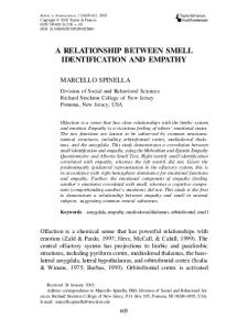
Our main interest variable is the log of total natural resources rents available from 1970 to 2005 for 15 different commodities. We also build three new indicators from natural resources rents according to the appropriability level. For this classification, we follow the standard classification on these topics used in the literature according SITC classification. We aggregate rents from gas, oil, hard coal, brown coal on a single variable (named rent 3) ; bauxite, copper, gold, iron, lead, nickel, phosphate, silver, tin, zinc in an another variable (named rent 6). A third variable is created with forest (named rent 4). We separate this one because it is the only natural resource which is renewable (see figure 4 and table 10 for some summary statistics).

.3 Density .2 .1 0

0

.1

Density .2

.3

F IGURE 4 – Natural Resources Rents Dispersion

10 15 Log Rent (Total)

20

25

0

5

10 15 Log Rent 4

20

25

5

10 15 Log Rent 3

20

25

0

5

10 15 Log Rent 6

20

25

Density .2 0

.1

Density .2 .1 0

3.2.2

0

.3

5

.3

0

Institutional Data

A new far-reaching literature uses institutional data. We notice that all these data are an institutional perception and not institutions themselves. The institutional perception is more volatile than institutions themselves. This precision explains why we can say that institutions change in a short period of time, given the currently common view of the persistence of institutional quality. We use different indicators to empirically test our theory through a panel data analysis. PolityIV provides a measure for political institutions from 1960 to 2005. We take Polity2 as a measure for political institutions from PolityIV. This one is computed by subtracting an autocracy score from a democracy score and measures a balance of the “Competitiveness of executive recruitment”, the “Openness of executive recruitment”, the “ Constraint on chief executive”, the “Competitiveness of political 16

participation” and the "Regulation of participation”. We use two synthetic indicators. First, The PRS Group has been producing the International Country Risk Guide (ICRG) since 1984. This provides a synthetic indicator that could be distinguished between political, economic and financial risks. This measurement ranges from 0 (Low Institutions) to 100 (Good Institutions). Second, Heritage provides an another synthetic indicator (heri) capturing the economic freedom (including trade freedom, business freedom and corruption by example) from 1995 to 2007 and is ranked from 0 (Weak Institutions) to 100 (Good Institutions). Kaufman’s data provides interesting details with indicators which are more precise than ICRG or Heritage. We use 5 variables : “Voice and Accountability” (VA) which measures political, civil and Human rights ; “Political Stability” (PS) which gives the probability to reverse a government ; “Government Effectiveness” (GE) is a quality government measurement ; “Rule of Law” (RL) and “Control of corruption” (CC). They range from -2.5 (Bad Institutions) to 2.5 (Good Institutions) and are available from 1996 to 2004. 18 These data are very helpful because it provides different measures according to various institutional characteristics and allows for the observation of whether natural resource’s impacts are the same through the institutional measure. Last, we use an another institutional measure linked to property rights (pr). It comes too from Heritage. It is ranked from 0 (Weak Institutions) to 100 (Good Institutions) and is available from 1995 to 2007. To check the robustness of our empirical work, we used some other variables which could influence the institutions. We have provided a list of these variables in the appendix.

4

Results and Estimation Procedures In this section we test equation 14. Each section uses different estimation procedures to provide

empirical proof of the theoretical conclusion.

4.1

Results with Fixed Effects Table 1 shows for the baseline results using a panel with country fixed effects. Some mains arguments

explain the choice of fixed effects. First, Hausman test indicates that the model with fixed effect is best than a model with random-effects. Second, it maximizes the number of observations. Last, fixed effects capture all time-invariant determinant of institutions as such geography (country size, access to sea, latitude...), history or colonial origin which are principal determinants of institutions building. Country fixed effects also control for the number of years that an economy has been resource dependent which 18. Data are missing for 1997, 1999, 2001.

17

could explain a part of the institutional quality. Alexeev and Conrad (2009) show that including GDP per capita leads to a misleading estimates of the effect of natural resources on institutional quality. The country fixed effects methodology avoid this problem capturing the initial level of development (e.g. GDP). With country fixed effects, we interpret our results as a within variation (i.e at the country level). We have 8 different institutional measure which are endogenously determined by natural resources rents. All equations, excepted specification (7), give the expected results, β1 > 0 and β2 < 0. These results seem to be robust in the majority of cases. This provides a support for our theoretical result. For low rent levels, the effect on the institutional level is positive and after the turning point, the effect is negative, producing the predicted inverted U-shape curve.

We calculate the turning point for each equation. It appears to be different according to the institutional nature which is measured. Voice and Accountability (equation 1) breaks up with a great amount of rents (turning point at 800 millions dollars) as Rule of Law (turning point at 26.7 millions dollars). The natural resources impact has a different intensity according to the institutional nature measured. The two lowest turning point is associated with the two measures of property rights (‘Rule of Law’ and ‘Property Rights’ from Heritage). Institutions which allow to respect property rights are the first to be deteriorate. The deterioration or the hijacking of property rights is one of the main tool to capture natural resources rents. As we show in table 11 (in appendix), turning points are not aberrant. According to the Voice and Accountability measure, Bahamas, Botswana or Ghana are in the increasing part of the relationship in 2005 and Algeria and Angola are in the decreasing part. In the same way, only 15% of countries of our sample in 2005 are in the increasing part of the relationship when we consider the Rule of Law measure.

The literature considers that if the quadratic terms are significant (positive or negative) we have a non linear effect (U-shaped or inverted U-shape curve respectively). Lind and Mehlum (2010) supply a new theory which allows us to confirm the non-linearity. Indeed they find that a significant quadratic term is too weak criteria. According to them, we must estimate if the turning point is in the data-range and test slopes on the interval’s beginning and ending. In our case (for an inverse U-shape), we must find for the lower bound, a positive slope and for the upper bound, a negative slope. They adopt a test which has been developed by Sasabuchi (1980). The Sasabuchi Test indicates whether we have an inverted U-Shape curve or not. Table 2 summarizes all the results with this methodology for the first eight specifications. Specifications (2), (3), (5), (6) and (8) are strongly significant and confirm natural resources non linear effect on 18

institutions with an inverted U-Shape curve. Specification (7) confirms the lack of effect with the global indicator from Heritage. Results for specifications (1) and (4) suggest some different interpretations. For these specifications, the higher bound of the confidence interval with Fieller method is very quite or higher at the higher bound of log rent’s interval. The turning point could be outside the data range even though Sasabuchi test is significant. But, if the turning point is near the higher bound of the log rent interval, the significance inverse hump shaped relationship is weak. Therefore, we could reconsider the natural resources positive effect on institution’s quality. The inverted U-shape curve is not always identified, and for some special institutional measure, we could only have a positive effect.

TABLE 1 – Natural Resources Impact on Institutional Quality with Fixed Effects Specifications

1

2

3

4

5

6

7

8

VA

RL

GE

CC

PS

pr

heri

icrg

LogRentt−1

0.210***

0.276***

0.190***

0.161***

0.222**

10.01***

0.864

(0.0558)

(0.0506)

(0.0600)

(0.0597)

(0.0885)

(1.765)

(0.848)

LogRent2t−1

-0.00512***

-0.00807***

-0.00511***

-0.00416**

-0.00665***

-0.353***

-0.0186

(0.00157)

(0.00142)

(0.00168)

(0.00166)

(0.00248)

(0.0494)

(0.0237)

Dep. Var.

LogRentt−3

6.059***

LogRent2t−3

-0.173***

(1.385)

(0.0404)

Observations

1085

1075

1074

1057

1066

1469

1467

2152

R-squared

0.02

0.035

0.011

0.008

0.008

0.067

0.002

0.009

Presence of inverse U-Shaped Turning Point :

Yes

Yes

Yes

Yes

Yes

Yes

No

Yes

800.9

26.7

119.6

240.1

10.6

1.5

-

17.51

(Millions Dollars) Note : Standard errors in parentheses with ∗∗∗ , ∗∗ and ∗ respectively denoting significance at the 1%, 5% and 10% levels. OLS regressions. All regressions included country fixed effects. Constant is not shown. VA : Voice and Accountability ; RL : Rule of Law ; GE : Government Effectiveness ; CC : Control of Corruption ; PS : Political Stability ; pr : Property Rights heri : Composite indicator from Heritage ; ICRG : Composite indicator from PRS Group.

19

TABLE 2 – Test for U-Shaped (Lind and Mehlum (2010)) Specifications :

(1)

(2)

(3)

(4)

(5)

(6)

(7)

(8)

Dep. Var. :

VA

RL

GE

CC

PS

pr

heri

icrg

Interval :

[6.36 ; 26.03]

[6.36 ; 26.03]

[6.36 ; 26.03]

[6.36 ; 26.03]

[6.36 ; 26.03]

[6.36 ; 26.03]

[6.36 ; 26.03]

[6.36 ; 26.03]

Slope at Lower Bound :

0.144∗∗∗

0.173∗∗∗

0.125∗∗∗

0.107∗∗∗

0.13∗∗∗

5.51∗∗

6.36

3.85∗∗∗

Slope at Upper Bound :

∗∗∗

∗∗∗

∗∗∗

∗∗

∗∗∗

-0.106

-2.94∗∗∗

∗∗

0.24

3.80∗∗∗

Sasabuchi Test for inverse U-shaped : Turning Point (Log Rent) : 95% confidence interval for extreme point :

-0.056

-0.143

∗∗∗

∗∗∗

1.94

5.24

-0.075

∗∗∗

2.43

-0.056

∗∗

1.44

∗∗∗

-0.124

-8.36

∗∗∗

2.37

4.77

20.50

17.1

18.6

19.3

16.7

14.2

23.2

17.51

[18.28 ; 26.14 ]

[15.73 ; 18.40]

[16.1 ; 22.73]

[16.30 ; 27.63]

[11.67 ; 19.82]

[12.48 ; 15.33]

[-Inf ; +Inf]

[16.15 ; 19.21]

Yes

Yes

Yes

Yes

Yes

Yes

No

Yes

(Fieller method ) Presence of inverse U-Shaped

Note : With ∗∗∗ , ∗∗ and ∗ respectively denoting significance at the 1%, 5% and 10% levels VA : Voice and Accountability ; RL : Rule of Law ; GE : Government Effectiveness ; CC : Control of Corruption ; PS : Political Stability ; pr : Property Rights heri : Composite indicator from Heritage ; ICRG : Composite indicator from PRS Group.

One concern of our first results is linked to the fact that one dollar of resource rent in US or China is not the same as it is in Kuwait or Botswana. The country fixed effects capture a part of this effect but in robustness check, we adjust our main interest variable for economy size. Using GDP level for each country introduces serious problem as treated before as the size of population has not. For each year, we compute natural resources rent per capita by devising the natural resources rent by the population. Our results are unchanged (table 13 in appendix).

4.2

Results with Random-effects We consider now a model with random-effects for four main reasons. First, the descriptive statistics

for the main variables indicate clearly that standard deviation “between” is bigger than “within”. Second, that most of the specifications have a weak time dimension. Third, many classical institutional determinants are mostly invariant. Fourth, for each specification, we make a Breusch Pagan Lagrange-multiplier test. In all our cases, random-effects are significant. These four reasons give a motivation to use GLS random-effect models. We include time invariant determinants of institutions commonly used in the literature like the distance to equator, the fraction of the population speaking European language or English, the rate secondary school enrollment for 1965 (see Alexeev and Conrad (2009)). For all specifications with random-effects, we observe the expected sign for β1 and β2 (table 3). We run again for all specifications the test from Lind and Mehlum (2010). This test confirms for all specifications, excepted specification (7), the presence of inverse U-shaped. 19 The control variables commonly used in the literature have the expected sign.

19. Results are not shown here but are available upon request.

20

Robustness Check The random-effects model allows to test the robustness of our conclusion using another determinants of institutions commonly used in the literature and if our results are not driven by some omitted variables. Table 4 provides a robustness check with ICRG used as the institutional measurement. The first specification is the baseline using panel data with random-effects. We introduce ethnic fractionalization, malaria in 1994 and the part of population that lived on a temperate zone in 1995. The estimated coefficients of these three variables are not significant and natural resources effects don’t vary. Ethnic fractionalization is insignificant as Alesina et al. (2003), Hodler (2006) found once when they controlled for distance to equator. We test the robustness of our results with civil war lagged for one year. It appears that civil war damages the institutional level but we still find that the natural resources have a non linear effect on institutional quality, but it is less significant. This point could be explained by the literature about the conflict, notably by Collier and Hoeffler (2004). They found that natural resource dependence increases probability of civil war because rents provide a financial opportunity for rebelion. Indeed, without natural resources dependence, the probability of civil war is near 0.5% and with a percentage of national income from primary commodity exports at 23%, the probability climbs to 26%. Fearon (2005) offers a new interpretation. He thinks that rebels could finance themselves with natural resources only marginally. The probability of civil war increases because there is an institutional degradation and the country chooses "extractive" institutions. 20 These authors found a negative relationship between natural resource and civil war which could explain our specification (4). To check the robustness of our results, we control for the geographic localization by regions. We test for 8 diverse areas but we present just two specifications (6) and (7). 21 However, in all cases, the natural resources effect is robust. The last two robustness checks concern legal origin matter. Again, we test for 4 diverse legal origins and we find, for each one, that the natural resource’s effect is robust. Specifications (8) and (9) show regressions with French and German legal Origin. Once again, we use our main interest variable adjusting for economy size. Our results are unchanged (table 14 in appendix). 20. Acemoglu et al. (2001) consider "extractive" institutions as a main cause of bad economic performance. 21. Others are available upon request

21

TABLE 3 – Natural Resources Impact on Institutional Quality with Random-Effects Specifications

(1)

(2)

(3)

(4)

(5)

(6)

(7)

(8)

Dep. Var.

VA

RL

GE

CC

PS

pr

heri

icrg

0.163***

0.261***

0.177***

0.210***

0.148*

6.068***

2.695***

(0.0627)

(0.0538)

(0.0620)

(0.0611)

(0.0891)

(1.919)

(0.875)

-0.00474***

-0.00786***

-0.00538***

-0.00648***

-0.00577**

-0.219***

-0.0781***

(0.00172)

(0.00147)

(0.00170)

(0.00167)

(0.00243)

(0.0526)

(0.0241)

LogRentt−1

LogRent2t−1

LogRentt−3

3.214**

LogRent2t−3

-0.0968**

(1.326)

(0.0378) Log GDP/cap 1990

Distance to Equator

Openness

Fraction European Speaking

Fraction English Speaking

Secondary Schooling 1965

0.106*

0.316***

0.317***

0.334***

0.216***

9.030***

3.474*** (1.130)

(0.0628)

(0.0579)

(0.0596)

(0.0572)

(0.0748)

(1.614)

0.240

1.281***

1.267***

1.338***

1.089*

0.722

-1.574

10.70

(0.473)

(0.437)

(0.448)

(0.430)

(0.560)

(12.05)

(8.522)

(7.091)

0.0315

0.0657

0.0535

0.0380

0.135**

1.408

0.542

0.661

(0.0494)

(0.0456)

(0.0468)

(0.0449)

(0.0585)

(1.260)

(0.891)

(0.738)

0.699***

0.128

0.226

0.142

0.468**

2.566

7.341***

2.300

(0.157)

(0.145)

(0.149)

(0.143)

(0.186)

(3.991)

(2.821)

(2.365)

-0.207

0.183

0.241

0.297

-0.0124

8.373

2.129

0.116

(0.251)

(0.232)

(0.238)

(0.229)

(0.298)

(6.396)

(4.522)

(3.937)

0.0230***

0.0107***

0.0100**

0.00986**

0.00892*

0.222**

0.0913

0.160**

(0.00440)

(0.00406)

(0.00417)

(0.00401)

(0.00523)

(0.112)

(0.0790)

(0.0671)

Log GDP/cap 1980

5.043*** (1.024)

Observations

713

713

710

704

711

1032

1032

1588

R-squared

0.72

0.8

0.8

0.82

0.66

0.49

0.62

0.71

Turning Point :

27.78

16.35

13.66

10.74

1.03

31

0.6

16

Yes

Yes

Yes

Yes

Yes

Yes

No

Yes

(Millions dollars) Presence of inverse U-Shaped (Method from Lind and Mehlum) Note : Standard errors in parentheses with ∗∗∗ , ∗∗ and ∗ respectively denoting significance at the 1%, 5% and 10% levels. OLS regressions. Constant is not shown. VA : Voice and Accountability ; RL : Rule of Law ; GE : Government Effectiveness ; CC : Control of Corruption ; PS : Political Stability ; pr : Property Rights heri : Composite indicator from Heritage ; ICRG : Composite indicator from PRS Group.

22

TABLE 4 – Robustness Check With ICRG Specifications :

(1)

(2)

(3)

(4)

(5)

(6)

(7)

(8)

(9)

Dep. Var. :

icrg

icrg

icrg

icrg

icrg

icrg

icrg

icrg

icrg

3.059∗∗

3.280∗∗

3.073∗∗

2.464∗

2.780∗∗

3.180∗∗

2.510∗

3.105∗∗

2.889∗∗

(1.312)

(1.314)

(1.314)

(1.295)

(1.326)

(1.292)

(1.283)

(1.305)

(1.297)

LogRent2t−3

-0.091∗∗

-0.099∗∗∗

-0.092∗∗

-0.075∗∗

-0.082∗∗

-0.096∗∗∗

-0.071∗

-0.091∗∗

-0.084∗∗

(0.037)

(0.038)

(0.037)

(0.037)

(0.038)

(0.037)

(0.036)

(0.037)

(0.037)

Log GDP/cap 1980

4.365∗∗∗

4.588∗∗∗

4.239∗∗∗

3.717∗∗∗

4.176∗∗∗

4.359∗∗∗

4.914∗∗∗

4.509∗∗∗

4.135∗∗∗

(1.004)

(1.056)

(1.062)

(0.915)

(1.017)

(0.948)

(0.938)

(0.988)

(0.966)

Distance to Equator

12.170∗

12.538∗

11.296

10.928∗

5.428

20.168∗∗∗

17.604∗∗∗

12.283∗

11.531∗

(6.825)

(7.398)

(7.212)

(6.154)

(8.744)

(6.802)

(6.414)

(6.688)

(6.540)

Openness

4.614∗∗∗

4.672∗∗∗

4.607∗∗∗

3.923∗∗∗

4.668∗∗∗

4.662∗∗∗

5.018∗∗∗

4.695∗∗∗

4.782∗∗∗

(1.119)

(1.199)

(1.119)

(1.154)

(1.119)

(1.107)

(1.107)

(1.115)

(1.112)

3.279

3.871

2.957

3.557∗

3.267

5.027∗∗

1.179

5.036∗∗

2.822

(2.238)

(2.421)

(2.392)

(2.022)

(2.230)

(2.162)

(2.134)

(2.349)

(2.152)

LogRentt−3

Fraction European Speaking

Fraction English Speaking

Secondary Schooling 1965

-0.469

-1.604

-0.316

-1.318

-0.577

-2.289

-0.187

-3.999

1.203

(3.875)

(4.036)

(3.915)

(3.491)

(3.839)

(3.679)

(3.533)

(4.156)

(3.767)

0.178∗∗∗

0.195∗∗∗

0.175∗∗∗

0.201∗∗∗

0.155∗∗

0.106

0.121∗

0.160∗∗

0.165∗∗∗

(0.066)

(0.068)

(0.067)

(0.060)

(0.069)

(0.066)

(0.063)

(0.065)

(0.064)

Ethnic Fractionalization

0.037 (0.033)

Malaria 94

-1.190 (3.022) -8.505∗∗∗

Civil War t-1

(0.901) Population Temperate Zone 95

4.879 (3.902) 9.038∗∗∗

East Asia and Pacific

(2.535) -8.432∗∗∗

Middle East and North Africa

(2.418) -3.624∗∗

French Legal Origin

(1.747) 9.698∗∗∗

German Legal Origin

(3.722) N

1564

1524

1564

1480

1561

1564

1564

1564

1564

R2

0.733

0.736

0.733

0.775

0.739

0.768

0.771

0.747

0.755

Yes

Yes

Yes

Yes

Yes

Yes

Yes

Yes

Yes

Presence of inverse U-Shaped (Method from Lind and Mehlum)

Note : Standard errors in parentheses with ∗∗∗ , ∗∗ and ∗ respectively denoting significance at the 1%, 5% and 10% levels OLS regressions. Random-effects used for each specification. Constant is not shown. ICRG : Composite indicator from PRS Group.

4.3

Results with the “Fixed Effects Vector Decomposition" Method The model with fixed effects and the one with random-effects are some limits. But Plümper and

Troeger (2007) provide a new methodology, Fixed Effects Vector Decomposition" (FEVD), which enables estimation of models with time-invariant variable with fixed effects and provide a new robustness check. The FEVD estimation procedure consists of a three-step estimation. The first step consists in estimating the fixed effects with a panel regression without time-invariant variable. The second step provides the regression of the fixed effects on the time-invariant variable using OLS. The residual part of this regression is the unexplainable part of fixed effects by the time-invariant variable. The third and last 23

step is an estimation of a pooled OLS that includes time-varying and time-invariant variables, and the unexplained part of fixed effects. Table 5 contains Fixed Effects Vector Decomposition, which assumes problems with a random-effect model, yields β1 > 0 and β2 < 0. The non-linearity effect of natural resources on institutional quality seems to be robust to the fixed effect, random-effests model or Fixed Effects Vector Decomposition methodology. TABLE 5 – Fixed Effects Vector Decomposition Specifications

(1)

(2)

(3)

(4)

(5)

(6)

(7)

(8)

Dep. Var.

VA

RL

GE

CC

pr

heri

PS

icrg

LogRentt−1

0.178∗∗∗

0.307∗∗∗

0.205∗∗∗

0.258∗∗∗

9.829∗∗∗

3.093∗∗∗

(0.0254)

(0.0241)

(0.0226)

(0.0291)

(0.650)

(0.272)

LogRent2t−1

-0.00398∗∗∗

-0.00896∗∗∗

-0.00577∗∗∗

-0.00738∗∗∗

-0.360∗∗∗

-0.0855∗∗∗

(0.000668)

(0.000616)

(0.000591)

(0.000755)

(0.0180)

(0.00732)

LogRentt−3

0.225∗∗∗

4.909∗∗∗

(0.0397)

(0.669)

LogRent2t−3

-0.00681∗∗∗

-0.150∗∗∗

(0.00105)

(0.0184)

0.916∗∗∗

8.327∗∗∗

Log GDP/cap 1990

Distance to Equator

Openness

0.0618∗∗∗

0.312∗∗∗

0.298∗∗∗

0.318∗∗∗

10.44∗∗∗

3.228∗∗∗

(0.00941)

(0.00827)

(0.00905)

(0.0107)

(0.317)

(0.121)

∗∗∗

-0.531

-2.270∗∗

0.0745

∗∗∗

1.113

∗∗∗

1.110

1.214

(0.0758)

(0.0610)

(0.0697)

(0.0652)

(2.395)

(1.016)

(0.110)

(1.634)

-1.21e-09

2.24e-10

3.29e-10

2.37e-09

-1.07e-07

1.23e-08

-4.73e-09

2.01e-08

(0.0119)

(0.00447)

(0.00670)

(0.00662)

(0.146)

(0.0777)

(0.00817)

(0.157)

∗∗∗

∗∗∗

∗∗

∗∗∗

0.0785

∗∗∗

0.180

0.110

∗∗∗

1.359

6.117

∗∗∗

0.669

(0.0226)

(0.0159)

(0.0211)

(0.0200)

(0.685)

(0.301)

(0.0322)

(0.568)

Fraction English Speaking

-0.216∗∗∗

0.212∗∗∗

0.253∗∗∗

0.297∗∗∗

10.50∗∗∗

2.923∗∗∗

0.0119

1.223

(0.0296)

(0.0394)

(0.0336)

(0.0279)

(1.194)

(0.465)

(0.0452)

(0.752)

Secondary Schooling 1965

0.0260∗∗∗

0.0120∗∗∗

0.0119∗∗∗

0.0115∗∗∗

0.152∗∗∗

0.0941∗∗∗

0.0123∗∗∗

0.154∗∗∗

(0.000607)

(0.000559)

(0.000633)

(0.000624)

(0.0250)

(0.00944)

(0.00109)

(0.0164)

0.209∗∗∗

5.495∗∗∗

Log GDP/cap 1980

Residuals

0.375

1.554∗∗∗

Fraction European Speaking

(0.0188)

(0.273)

1∗∗∗

1∗∗∗

1∗∗∗

1∗∗∗

1∗∗∗

1∗∗∗

1∗∗∗

1∗∗∗

(0.0154)

(0.0142)

(0.0186)

(0.0158)

(0.0180)

(0.0124)

(0.0233)

(0.0281)

Observations

713

713

710

704

1032

1032

653

1588

R2

0.95

0.97

0.96

0.96

0.88

0.92

0.91

0.74

Turning Point :

5087

27.5

53.75

38.64

0.85

71.12

15.4

12.48

Yes

Yes

Yes

Yes

Yes

Yes

Yes

Yes

(Millions dollars) Presence of inverse U-Shaped (Method from Lind and Mehlum) Note : Standard errors in parentheses with ∗∗∗ , ∗∗ and ∗ respectively denoting significance at the 1%, 5% and 10% levels. VA : Voice and Accountability ; RL : Rule of Law ; GE : Government Effectiveness ; CC : Control of Corruption ; PS : Political Stability ; pr : Property Rights heri : Composite indicator from Heritage ; ICRG : Composite indicator from PRS Group.

24

4.4

Results for Different Turning Points One of our main predictions is that the turning point should be different for different countries de-

pending on institutional quality (see fig. 3). We test this prediction using ‘Rule of Law’ from Kaufmans’ data. We choose this proxy because it captures a key aspect of institutions in the management of natural resources. We run 4 regressions to test this prediction with random-effects(table 6). In specification (1) and (2), we split the sample into two parts according to the institutional level at the initial period. We take the institutional level mean in 1996 for each measure (the first year available for World Bank data). Specification (1) and (2) show that the turning point is different. The non-linearity effect is confirmed by the method from Lind and Mehlum (2010). Countries with a higher initial institutional level than the mean (specification 1) have a turning point at 63.1 millions dollars whereas countries with a lower initial institutional level than the mean have a turning point at 23.9 millions dollars. The turning point for countries with an initial institutional level superior to the mean is higher than the turning point for countries with an initial institutional level lower to the mean. We split also our sample in two part depending if country belongs to OECD or not. We show with an alternative specification that OECD countries have a higher turning point than non-OECD countries. The negative effect of natural resources on institutions for OECD appears with higher level of natural resources rent than for non-OECD countries. All these results are robust to the inclusion of country fixed effects (results available upon request). To provide additional proof we carry out a simultaneous quantile regression (Table 7). This methodology considers the error correlation between different quantiles. It enables comparison between coefficients in different quantiles (Koenker and Hallock (2001)). In our case, it allows for an observation of the evolution and the intensity of the impact from β1 to β2 . We split the sample into seven groups according to the Polity 2 measurement. 22 It appears clearly that the turning point increases with quantiles. The higher the quantile is, the higher the turning point. This means that natural resources’ positive impacts prevail less for a country with weak institutions than for a country with a high institutional level. Intensity for β1 and β2 between specifications (5) and (6) fail. We test if β1 between equations (5) and (6) are significantly different. We cannot reject the hypothesis according to which β1 ’s in each equations are equal. It allows to minimize the turning point for specification (6) and where the turning point is lower for the last quantile than for the next to last quantile . We also observe 22. We use Polity IV (political institution measure) for two mains reasons. First this index measure the political side of national institutions which completes the measure of ‘political stability’ from Kaufman’s data. Second, it’s the only one institutional measure where data are available for a large time period (since 1960).

25

that, for higher quantiles, the model’s power of explanation is reduced. Indeed, countries with a high institutional level are less influenced by rents or by the Distance to Equator, which are significant for the first four quantiles. Table 7 confirms one of our predictions about the different turning points according to the institutional level. TABLE 6 – Diverse Turning Point for Rule of Law Specifications

(1)

(2)

(3)

(4)

Dep. Var.

RL

RL

RL

RL

0.378***

0.206***

0.214**

0.309***

(0.0952)

(0.0681)

(0.0836)

(0.0976)

-0.0105***

-0.00607***

-0.00674***

-0.00821***

(0.00242)

(0.00195)

(0.00234)

(0.00251)

0.421***

0.0414

0.271***

0.555**

(0.0737)

(0.0796)

(0.0651)

(0.217)

LogRentt−1

LogRent2t−1

Log GDP/cap 1990

0.762

0.559

0.748

0.978

(0.531)

(0.556)

(0.511)

(1.045)

0.209*

0.0583

0.0681

0.109

(0.107)

(0.0438)

(0.0481)

(0.205)

0.247

0.231

0.102

0.320

(0.162)

(0.188)

(0.172)

(0.217)

Fraction English Speaking

0.0810

0.266

-0.254

0.340

(0.231)

(0.390)

(0.325)

(0.246)

Secondary Schooling 1965

0.00552

0.0106

0.0126**

0.00820

(0.00393)

(0.00645)

(0.00497)

(0.00611)

Distance to Equator

Openness

Fraction European Speaking

Observations

291

422

500

109

R2

0.76

0.27

0.49

0.67

RL96 > Mean RL96

RL96 < Mean RL96

Non OECD

OECD

63.1

23.9

7.6

152.1

Yes

Yes

Yes

Yes

Sample

Turning Point : (Millions dollars) Presence of inverse U-Shaped (Method from Lind and Mehlum)

Note : Standard errors in parentheses with ∗∗∗ , ∗∗ and ∗ respectively denoting significance at the 1%, 5% and 10% levels. OLS regressions. Random-fixed effects used for all columns. Constant is not shown. RL : Rule of Law.

26

TABLE 7 – Impacts on Polity IV With Quantiles Specifications : Dep. Var. : Quantiles : LogRentt−1

(1)

(2)

(3)

(4)

(5)

(6)

pol2

pol2

pol2

pol2

pol2

pol2

q15

q30

q45

q60

q75

q90

0.556∗

0.671∗∗∗

0.915∗∗

1.80∗∗∗

1.121∗

0.708∗∗∗

(0.323)

(0.192)

(0.441)

(0.284)

(0.654)

(0.213)

∗

∗∗∗

∗

∗∗∗

∗

-0.019∗∗∗

LogRent2t−1

-0.023

(0.012)

(0.006)

(0.015)

(0.008)

(0.016)

(0.006)

Log GDP/cap 1962

-0.876∗∗

0.457

0.603

0.805∗∗

-0.130

0.475∗∗∗

(0.428)

(0.414)

(0.804)

(0.348)

(0.212)

(0.136)

Distance to Equator

Openness

-1.078

-0.025

-4.506

∗∗∗

-0.028

∗∗∗

-6.591

-0.048

∗∗∗

-5.270

-0.029

0.230

-0.333

(1.107)

(1.125)

(1.584)

(1.129)

(0.898)

(0.252)

-0.279

-0.781∗∗∗

-0.516

-0.944∗

0.177

-0.112

(0.254)

(0.260)

(0.643)

(0.527)

(0.405)

(0.143)

Fraction European Speaking

5.098∗∗∗

6.589∗∗∗

8.290∗∗∗

5.015∗∗∗

3.783∗∗∗

0.759∗∗∗

(1.018)

(0.726)

(0.725)

(0.469)

(0.499)

(0.123)

Fraction English Speaking

7.406∗∗∗

-1.091∗

-3.962∗∗∗

-3.385∗∗∗

-2.486∗∗∗

-0.572∗∗∗

(2.677)

(0.652)

(0.763)

(0.451)

(0.506)

(0.172)

Secondary Schooling 1965

0.143∗∗∗

0.225∗∗∗

0.217∗∗∗

0.184∗∗∗

0.121∗∗∗

0.023∗∗∗

(0.037)

(0.010)

(0.031)

(0.013)

(0.016)

(0.009)

0.1992

0.3557

0.3780

0.2871

0.1813

0.0605

0.17

0.67

12.47

139

247.7

123.47

2

R

Turning Point (Millions Dollars)

Note : Standard errors in parentheses with ∗∗∗ , ∗∗ and ∗ respectively denoting significance at the 1%, 5% and 10% levels. Pol2 : Polity IV

4.5

Results According to the Appropriability’s Level Table 8, with random-effects, illustrates another theoretical prediction about the appropriability level.

The effect on institutions is not the same according to the natural resources type. Specification (1) is the baseline and gives a non linear effect on ICRG for a global rent (randomeffects is used). Specifications (2) to (4) take into account the different natural resources types. The effects are different. Indeed, specification (2) indicates a U-Shape which is confirmed by Lind and Mehlum (2010)’s theory even though Fieller interval is near the lower bound of the dataset. With this closeness between the turning point and the Fieller interval, if the negative effect exists, we quickly have a positive effect. This particular case could be explained by the nature of the natural resource. In fact, the variable Rents 4 includes only a measurement for forests. Although it is a renewable resource and all our predictions and the literature about this topic are about non-renewable natural resources. For products ranked in class 3, we again find the inverted U-shape curve which is confirmed by Lind and Mehlum (2010)’s test. On the other hand, in specification (4), we find only a negative effect. Specifications (5) and (6)

27

refine this assumption. If we split the sample between OECD Countries and non-OECD countries, we observe two distinct effects. For OECD countries, we find again an inverted U-Shape curve which is confirmed by the test from Lind and Mehlum (2010). For non-OECD countries, we have just a negative effect. According to the natural resource type, the effect on institutional level measured by ICRG could be different. If we do not have an inverted U-Shape curve, it appears that the effect is negative which is developed by the literature on this topics. We explain this permanent negative effect by a very weak institutional quality which is not able to bear natural resource rents.

28

TABLE 8 – Impact on Institutional Quality According Natural Resource Types Specifications

(1)

(2)

(3)

(4)

(5)

(6)

Dep. Var.

icrg

icrg

icrg

icrg

icrg

icrg

-2.184*

6.344***

-2.812*

(1.249)

(2.210)

(1.482)

0.0546

-0.193***

0.0761

(0.0396)

(0.0654)

(0.0477)

LogRentt−3

3.214**

LogRent2t−3

-0.0968**

(1.326)

(0.0378) LogRent4t−3

-11.18***

LogRent42t−3

0.476***

(3.096)

(0.0963) LogRent3t−3

2.716* (1.573)

LogRent32t−3

-0.110** (0.0436)

LogRent6t−3

LogRent62t−3

Log GDP/cap 1980

5.043***

11.58***

5.483***

4.244***

6.981*

3.610**

(1.024)

(1.961)

(1.156)

(1.259)

(3.587)

(1.435)

10.70

-3.100

4.782

7.976

1.611

0.856

(7.091)

(13.00)

(7.393)

(7.453)

(16.07)

(9.269)

Distance to Equator

Openness

Fraction European Speaking

1.088

-0.704

0.581

0.500

0.565

(0.857)

(0.798)

(0.757)

(3.198)

(0.838)

2.300

-2.710

2.735

2.445

2.985

1.126

(2.365)

(4.832)

(2.676)

(2.538)

(3.188)

(3.215)

0.116

-175.0*

2.517

-0.156

0.937

-2.589

(3.937)

(90.17)

(4.278)

(4.244)

(3.386)

(7.693)

0.160**

-0.0681

0.152**

0.247***

0.0975

0.244**

(0.0671)

(0.108)

(0.0728)

(0.0717)

(0.101)

(0.101)

Fraction English Speaking

Secondary Schooling 1965

0.661 (0.738)

Observations

1588

566

1157

1277

298

979

R2

0.71

0.49

0.67

0.70

0.51

0.32

Turning Point :

16.03

0.13

2.21

-

13.25

-

Yes

No

Yes

No

Yes

No

(Millions dollars) Presence of inverse U-Shaped (Method from Lind and Mehlum) Note : Standard errors in parentheses with ∗∗∗ , ∗∗ and ∗ respectively denoting significance at the 1%, 5% and 10% levels. Following SITC classification : LogRent3t−3 : Gas, oil, hard coal, brown coal. LogRent4t−3 : Forest. LogRent6t−3 : Bauxite, copper, gold, iron, lead, nickel, phosphate, silver, tin, zinc. OLS regressions. Random-fixed effects used for all columns. Constant is not shown. icrg : Composite indicator from PRS Group.

29

5

Conclusion This paper examines the natural resource’s effect on institutions. Our conclusion about a hump sha-

ped or negative effects on institutions partially confirm the view provided by various authors such Ross (2001a), Leite and Weidmann (1999), Sala-i Martin and Subramanian (2003), Isham et al. (2005), Bulte et al. (2004) . But these authors do not contemplate a positive effect. Brunnschweiler (2008) finds that “Natural resource abundance does not necessarily lead to worse institutions...”. Moreover, why has Norway strong institutions whereas Nigeria has weak institutions ? Our results offer a response to this puzzle. Each country has a structural institutional capacity to bear some natural resource rent. National institutions determine a threshold in the amount of natural resources and beyond this point the resource’s positive impact on institutions becomes negative. Further interesting research could take into account this finding about the non linear effect to explain another discord within the literature on rent-seeking. Indeed there is a large debate on the natural resource’s impact on growth. Since Sachs and Warner (1995), many authors found a negative relationship but some authors (Brunnschweiler, 2008; Alexeev and Conrad, 2009) reject this negative relationship. Mehlum et al. (2006) provide a first response to this debate : natural resources could be a blessing for countries with good institutions or a curse if a country has bad institutions. But authors do not weigh the natural resources non linear effect on institutions. Our findings provide one complementary explanation to this debate.

30

Technical Appendix 5.1

Proof for s value To find s, we must take into account the shares of resources for each group (Mehlum et al., 2006).

Grabbers use their entire effort for the rent-seeking activity, that’s why we have a proportion (1 − α) with the effort normalized to one. The producer’s effort is lower than the grabber’s effort and depends on the institutional level. The better the institutional quality, the more efficient is the effort to capture a part of rent. The sum of shares cannot exceed one. It comes : αλs + (1 − α)s ≤ 1. If the constraint is saturated (no waste), it is implying : s =

5.2

1 (1−α)+αλ

Proof for π First : π = y(1 − β1 ) − F then we have : nf π = ynf (1 − β1 ) − nf F . We express GDP like : V X 1 qi (pi − ci ) Y = L + N (απf + πg (1 − α)) = L + N απ + γi

(15)

i=1

β(L−nf F ) β(M −nf )+nf . We have an expression β(L−F M )−L β(M −nf )+nf

Which gives : nf π = M y −L. With a factorization, we found : y = for π that does not depend on the institutional level : π =

If πf > πg then, P (α − 1)N π + Vi=1 γ1i qi (pi − ci ) λ> PV 1 i=1 γi qi (pi − ci ) + αN π

(16)

and if α =1, PV

1 i=1 γi qi (pi − ci ) 1 i=1 γi qi (pi − ci ) + N π

λ > PV

(17)

If πf = πg then,

α=

(λ − 1)

PV

1 i=1 γi qi (pi

− ci ) + N π

(1 − λ)N π

31

(18)

5.3

The turning point A On the point A, we have πf = πg and no grabbers in the economy (α = 1). If the price increasing,

we can stay on the same point A and have some improvements on the institutional quality : PV

1 i=1 γi qi (pi − ci ) s PV 1 i=1 γi qi (pi − ci ) + N π N qi γi N π >0 P ( Vi=1 γ1i qi (pi − ci ) + αN π)2

λ=

δλ = δpi

s N

with the assumption that π > 0.

32

(19) (20)

Empirical Appendix TABLE 9 – Sample of Countries Albania

Bangladesh

Cuba

El Salvador

Germany

Korea North

Morocco

New Caledonia

Sierra Leone

Syrian

UAE

Algeria

Barbados

Cyprus

Eritrea

Haiti

Korea South

Mozambique

New Zealand

South Africa

Taiwan

Uruguay

Argentina

Belarus

Czech Rep.

Estonia

Hungary

Kazakhstan

Myanmar

Niger

Spain

Thailand

Uzbekistan

Australia

Belgium

Cambodia

Ethiopia

Honduras

Kuwait

Macedonia.

Nigeria

Suriname

Turkey

Venezuela

Austria

Benin

Cameroon

Finland

India

Kyrgyz Rep.

Madagascar

Oman

Sweden

Tajikistan

Vietnam

Afghanistan

Bhutan

Central Afr. Rep.

France

Indonesia

Lao

Malawi

Pakistan

Saudi Arabia

Tanzania

Yugoslavia Yemen

Angola

Bosnia

Chad

Fiji

Iran

Lebanon

Mauritius

Papua New Guinea

Senegal

Togo

Armenia

Brunei

Comoros

Ghana

Ireland

Lesotho

Moldova

Peru

Slovak Rep.

Tonga

Zaire

Azerbaijan

Burkina Faso

Costa Rica

Greece

Israel

Liberia

Monaco

Philippines

Slovenia

Trinidad and Tobago

Zambia

Bolivia

Burundi

Ivory Coast

Guatemala

Italy

Libya

Namibia

Poland

Solomon Is.

Tunisia

Zimbabwe

Botswana

Canada

Croatia

Guinea

Iraq

Lithuania

Nauru

Portugal

Somalia

Turkmenistan

Brazil

Chile

Dominican Rep

Guyana

Jamaica

Malaysia

Nicaragua

qatar

Sri Lanka

Uganda

Bulgaria

China

Denmark

Gabon

Japan

Mauritania

Norway

Romania

Sudan

United Kingdom

Bahamas. The

Colombia

Ecuador

Gambia

Jordan

Mexico

Nepal

Russia

Swaziland

United States

Bahrain

Congo

Egypt.

Georgia

Kenya

Mongolia

Netherlands

Rwanda

Switzerland

Ukraine

Note : Countries for specification 1 in table 1. Regression with country fixed effects.

TABLE 10 – Summary Statistics for Natural Resources Rents (by year, in millions dollars) Percentiles

Total Rent

Rent 3

Rent 4

Rent 6

p10

36

0.6

2.4

0.5

p25

100

8.5

18.1

10

p50

641

266

78

38

p75

4511

2905

245

203

p90

12 638

8906

709

1460

mean

136

132

61

32

Following SITC classification : Rent 3 : Gas, oil, hard coal, brown coal. Rent 4 : Forest. Rent 6 : Bauxite, copper, gold, iron, lead, nickel, phosphate, silver, tin, zinc.

33

TABLE 11 – Example of countries by deciles (in millions of dollars) Déciles

Rentes

Example of countries (2005)

p10

10.6

Bahamas, Benin, Central Afr. Rep., Gambia, Mozambique

p25

47

Armenia, Belgium, Burkina Faso, Georgia, Senegal, Uruguay

p50

400

Albania, Botswana, Burundi,

p75

4 370

p90

19 300

Mean

7 680

Finland, Ghana, Morocco, Spain, Somalia, Togo Bahrain, Bolivia, Cameroon, Chad, Denmark, Gabon, Ireland, Ivory Coast, Sudan, Tunisia, Uganda Algeria, Angola, Azerbaijan, Brazil, Canada, Iran, Irak, Kuwait, Malaysia, Nigeria, Norway, Saudi Arabia, South Africa, USA, Venezuela

TABLE 12 – Variables and Sources Variable

Definition

Source

Log GDP/cap

Log of GDP per capita. GDP is measured in constant dollar for the year 2000

The World Bank

Openness

It is the sum between exportations and importations for a country for one year

Dataset from Robert Feenstra

divised by GDP Distance to Equator

We calculate the distance for each country such as

The World Bank

Distance to Equator = abs(Latitude)/90

and my own calculation

Fraction European/English

It is the fraction of the population speaking English

Hall and Jones (1999)

Speaking

and the fraction speaking one of the major languages of Western Europe : English, French, German, Portuguese, or Spanish

Secondary Schooling 1965

The rate of Secondary Schooling Enrollment for 1965

The World Development Indicator

Ethnic Fractionalization

Index of Ethnic Fractionalization.

Alesina et al. (2003)

It is ranking from 0 (least fractionalized) to 1 (extremely fractionalized) Malaria 1994

Percentage of population which could be infect by Malaria

Dataset from A.Shleifer

Population Temperate Zone 1995

Part of population living in temperate zone

Dataset from A.Shleifer

Civil War

It is a binomial variable coded 1 if there are at least 1000 deaths by year.

Correlate of War (COW)

This civil war must be an organized military act and dummy doesn’t take into account “external war’ and “extra-systemic war” Geographical Variable

Middle East and North Africa, East Asia and Pacific

The World Bank

Legal Origin

We distinguish five diverse legal Origins :

The World Bank

British, French, Socialist, German, Scandinavian. Dummy Income Level

We have six dummies to narrow countries through our income : low, lower-middle, upper-middle, highoecd, high non oecd and developing

34

The World bank

TABLE 13 – Natural Resources Impact per Capita on Institutional Quality with Fixed Effects Specifications Dep. Var.

LogRentt−1 per capita

LogRent2t−1 per capita

1

2

3

4

5

6

7

8

VA

RL

GE

CC

PS

pr

heri

icrg

0.103***

0.129***

0.102***

0.0834***

0.0699

2.948***

0.363

(0.0301)

(0.0279)

(0.0314)

(0.0322)

(0.0475)

(1.031)

(0.487)

-0.00405**

-0.00763***

-0.00532***

-0.00410**

-0.00464*

-0.281***

-0.00990

(0.00170)

(0.00158)

(0.00178)

(0.00180)

(0.00269)

(0.0577)

(0.0272)

LogRent2t−3 per capita

4.966***

LogRent2t−3 per capita

-0.373***

(0.610)

(0.0369)

Observations

1047

1044

1041

1028

1034

1437

1436

2086

R-squared

0.017

0.026

0.012

0.008

0.003

0.033

0.001

0.055

Note : Standard errors in parentheses with ∗∗∗ , ∗∗ and ∗ respectively denoting significance at the 1%, 5% and 10% levels. OLS regressions with countries fixed effects. All regressions included country fixed effects. Constant is not shown. VA : Voice and Accountability ; RL : Rule of Law ; GE : Government Effectiveness ; CC : Control of Corruption ; PS : Political Stability ; pr : Property Rights heri : Composite indicator from Heritage ; icrg : Composite indicator from PRS Group.

TABLE 14 – Natural Resources per Capita Impact on Institutional Quality Specifications Dep. Var.

LogRentt−1 per capita

LogRentt−1 per capita

Log GDP/cap 1990

Distance to Equator

Openness

Fraction European Speaking

Fraction English Speaking

Secondary Schooling 1965

1

2

3

4

5

6

7

8

VA

RL

GE

CC

PS

pr

heri

icrg

0.0713**

0.104***

0.0815**

0.0943***

0.00980

1.133

0.946**

(0.0331)

(0.0285)

(0.0326)

(0.0323)

(0.0477)

(1.019)

(0.462)

-0.00482***

-0.00749***

-0.00612***

-0.00683***

-0.00369

-0.182***

-0.0685***

(0.00186)

(0.00160)

(0.00183)

(0.00181)

(0.00267)

(0.0572)

(0.0260)

0.115*

0.328***

0.334***

0.344***

0.216***

9.594***

3.638***

(0.0623)

(0.0577)

(0.0587)

(0.0586)

(0.0788)

(1.608)

(1.119)

0.135

1.102**

1.116**

1.178***

0.883

-7.626

-3.195

1.427

(0.465)

(0.431)

(0.436)

(0.437)

(0.584)

(11.84)

(8.392)

(7.027)

0.0358

0.0767*

0.0625

0.0484

0.153**

1.984

0.635

0.586

(0.0483)

(0.0448)

(0.0453)

(0.0453)

(0.0606)

(1.230)

(0.874)

(0.716)

0.680***

0.100

0.201

0.116

0.454**

1.791

7.104**

0.230

(0.154)

(0.143)

(0.144)

(0.144)

(0.193)

(3.911)

(2.773)

(2.326)

-0.180

0.227

0.287

0.337

0.0366

10.94*

2.571

4.927

(0.247)

(0.229)

(0.232)

(0.232)

(0.310)

(6.288)

(4.453)

(3.896)

0.0235***

0.0116***

0.0104***

0.0106***

0.0104*

0.256**

0.0975

0.106

(0.00429)

(0.00398)

(0.00403)

(0.00403)

(0.00540)

(0.109)

(0.0774)

(0.0651)

LogRentt−3 per capita

2.704***

LogRentt−3 per capita

-0.233***

Log GDP/cap 1980

7.774***

(0.636)

(0.0388)

(1.061)

Observations

713

713

710

704

711

1032

1032

1588

R-squared

0.72

0.81

0.81

0.82

0.6

0.7

0.51

0.73

Note : Standard errors in parentheses with ∗∗∗ , ∗∗ and ∗ respectively denoting significance at the 1%, 5% and 10% levels. OLS regressions. All regressions included country fixed effects. Constant is not shown. VA : Voice and Accountability ; RL : Rule of Law ; GE : Government Effectiveness ; CC : Control of Corruption ; PS : Political Stability ; pr : Property Rights heri : Composite indicator from Heritage ; icrg : Composite indicator from PRS Group.

35

Références Acemoglu, D. (2006, December). “A Simple Model of Inefficient Institutions”. Scandinavian Journal of Economics 108(4), 515–546. Acemoglu, D. (2008). Introduction to Modern Economic Growth. Princeton University, Princeton, NJ. Acemoglu, D., S. Johnson, and J. A. Robinson (2001, December). “The Colonial Origins of Comparative Development : An Empirical Investigation”. American Economic Review 91(5), 1369–1401. Acemoglu, D., S. Johnson, and J. A. Robinson (2002, February). “An African Success Story : Botswana”. CEPR Discussion Papers 3219, C.E.P.R. Discussion Papers. Acemoglu, D. and J. A. Robinson (2007, March). “Persistence of Power, Elites and Institutions”. NBER Working Papers 12108, National Bureau of Economic Research, Inc. Aghion, P., A. Alesina, and F. Trebbi (2004, May). “Endogenous Political Institutions”. The Quarterly Journal of Economics 119(2), 565–611. Alesina, A., A. Devleeschauwer, W. Easterly, S. Kurlat, and R. Wacziarg (2003, June). “ Fractionalization”. Journal of Economic Growth 8(2), 155–94. Alexeev, M. and R. Conrad (2009, 02). The elusive curse of oil. The Review of Economics and Statistics 91(3), 586–598. Andersen, J. J. and S. Aslaksen (2008, October). Constitutions and the resource curse. Journal of Development Economics 87(2), 227–246. Anderson, J. E. and D. Marcouiller (2002, May). Insecurity and the pattern of trade : An empirical investigation. The Review of Economics and Statistics 84(2), 342–352. Beblawi, H. and G. Luciani (1987). The Rentier State. Routledge. Berkowitz, D., J. Moenius, and K. Pistor (2006, 08). Trade, law, and product complexity. The Review of Economics and Statistics 88(2), 363–373. Blume, L. E. and S. N.Durlauf (2001). “The Interactions-Based Approach to Socioeconomic Behavior”. In S.N Durlauf and H.P Young (eds.) “Social Dynamics". Washington, DC :Brookings Institutions Press, 15–44.

36

Bohn, H. and R. T. Deacon (2000, June). Ownership risk, investment, and the use of natural resources. American Economic Review 90(3), 526–549. Boschini, A. D., J. Pettersson, and J. Roine (2007, 09). “Resource Curse or Not : A Question of Appropriability”. Scandinavian Journal of Economics 109(3), 593–617. Brock, W. A. and S. N. Durlauf (2001, April). “Discrete Choice with Social Interactions”. Review of Economic Studies 68(2), 235–60. Brunnschweiler, C. N. (2008). “Cursing the blessings ? Natural resource abundance, institutions, and economic growth”. World Development 36(3), 399–419. Brunnschweiler, C. N. and E. H. Bulte (2008). “The resource curse revisited and revised : A tale of paradoxes and red herrings”. Journal of Environmental Economics and Management. Bulte, E. H., R. Damania, and R. T. Deacon (2004). “Resource Abundance, Poverty and Development”. Technical report. Collier, P. and A. Hoeffler (2004, October). “Greed and grievance in civil war”. Oxford Economic Papers 56(4), 563–595. Collier, P. and A. Hoeffler (2005). “Resource Rents, Governance and Conflict”. Journal of Conflict Resolution 49, 625–633. Congdon Fors, H. and O. Olsson (2007, November). Endogenous institutional change after independence. European Economic Review 51(8), 1896–1921. Cotet, A. and K. K. Tsui (2010, March). Resource curse or malthusian trap ? evidence from oil discoveries and extractions. Working papers, Ball State University, Department of Economics. Do and A. Levchenko (2007, February). “Trade, inequality, and the political economy of institutions”. Policy Research Working Paper Series 3836, The World Bank. Easterly, W. and R. Levine (2003, January). “Tropics, germs, and crops : how endowments influence economic development”. Journal of Monetary Economics 50(1), 3–39. Engerman and Sokoloff (1997). “Factor Endowments, Institutions and Differential Paths of Growth Among New World Economies : A view from Economic Historians of the United States”. in Haber (ed.) How Latin America Fell Behind Stanford : Stanford University Press.

37

Fearon, J. D. (2005). “Primary Commodity Exports and Civil War”. Journal of Conflicts Resolution 49(4), 483–507. Frankel, J. A. (2010, March). The natural resource curse : A survey. NBER Working Papers 15836, National Bureau of Economic Research, Inc. Frankel, J. A. and D. Romer (1999, June). Does trade cause growth ? American Economic Review 89(3), 379–399. Gylfason, T. (2001, May). Natural resources, education, and economic development. European Economic Review 45(4-6), 847–859. Haber, S., N. Maurer, and A. Razo (2003, March). When the law does not matter : The rise and decline of the mexican oil industry. The Journal of Economic History 63(1). Hall, R. E. and C. I. Jones (1999, February). “Why Do Some Countries Produce So Much More Output Per Worker Than Others ?”. The Quarterly Journal of Economics 114(1), 83–116. Hausman, J. A. and W. E. Taylor (1981). Panel data and unobservable individual effects. Econometrica 49(6), 1377–1398. Hodler, R. (2006, August). “The curse of natural resources in fractionalized countries”. European Economic Review 50(6), 1367–1386. Isham, J., M. Woolcock, L. Pritchett, and G. Busby (2005). “The Varieties of Resource Experience : Natural Resource Export Structures and the Political Economy of Economic Growth”. World Bank Economic Review 19(2), 141–174. Knack, S. and P. Keefer (1995). “Institutions and Economic Performance : Cross-Section Country Tests Using Alternative Institutional Mesures”. Economics and Politics 7, 207–227. Koenker, R. and K. F. Hallock (2001, Fall). “Quantile Regression”. Journal of Economic Perspectives 15(4), 143–156. Leite, C. and J. Weidmann (1999, July). “Does Mother Nature Corrupt - Natural Resources, Corruption, and Economic Growth”. IMF Working Papers 99/85, International Monetary Fund. Lind, J. T. and H. Mehlum (2010, 02). With or without u ? the appropriate test for a u-shaped relationship. Oxford Bulletin of Economics and Statistics 72(1), 109–118.

38

Mehlum, H., K. Moene, and R. Torvik (2006, 01). “Institutions and the Resource Curse”. Economic Journal 116(508), 1–20. Murphy, K. M., A. Shleifer, and R. W. Vishny (1989, October). “Industrialization and the Big Push”. Journal of Political Economy 97(5), 1003–26. North, D. C. (1994, June). “Economic Performance through Time". American Economic Review 84(3), 359–68. Plümper, T. and V. Troeger (2007). Efficient estimation of time-invariant and rarely changing variables in finite sample panel analyses with unit fixed effects. Political Analysis 15(2), 124–139. Rigobon, R. and D. Rodrik (2005). ‘Rule of Law, Democracy, Openness and Income : Estimating the Interrelationships”. Economic of Transition 9, 131–65. Rodrik, D., A. Subramanian, and F. Trebbi (2004). “Institutions Rule : The Primacy of Institutions Over Geography and Integration in Economic Development”. Journal of Economic Growth 9(2), 131–165. Ross, M. L. (2001a). “Does Oil hinder Democracy ?”. World Politics 53(3), 325–361. Ross, M. L. (2001b). “Extractive Sectors and the Poor”. Oxfam America Report. Sachs, J. D. and A. M. Warner (1995, December). “Natural Resource Abundance and Economic Growth”. NBER Working Papers 5398, National Bureau of Economic Research, Inc. Sala-i Martin, X. and A. Subramanian (2003, June). “Addressing the Natural Resource Curse : An Illustration from Nigeria”. NBER Working Papers 9804, National Bureau of Economic Research, Inc. Scheinkman, J. A. “Social Interactions”. Technical report, New Palgrave Dictionary of Economics and Law. Stijns, J.-P. (2003, May). “An Empirical Test of the Dutch Disease Hypothesis using a Gravity Model of Trade”. International Trade 0305001, EconWPA. Tornell, A. and P. R. Lane (1999, March). “The Voracity Effect”. American Economic Review 89(1), 22–46. Torvik, R. (2002, April). “Natural resources, rent seeking and welfar”. Journal of Development Economics 67(2), 455–470. Tsui, K. (2011, March). More oil, less democracy : Evidence from worldwide crude oil discoveries. Economic Journal 121(551), 89–115. 39

Acknowledgements : We are grateful to Lisa Anouliés, Rémi Bazillier, Daniel Berkowitz, Jerome Hericourt, Thierry Mayer, Marc Sangnier, Farid Toubal, Julien Vauday and Thierry Verdier for their constructive and helpful comments. All remaining errors are obviously ours.

40