Reinforcement Learning with Exploration Stuart Ian Reynolds A thesis submitted to The University of Birmingham for the degree of Doctor of Philosophy

School of Computer Science The University of Birmingham Birmingham B15 2TT United Kingdom December 2002

Abstract Reinforcement Learning (RL) techniques may be used to nd optimal controllers for multistep decision problems where the task is to maximise some reward signal. Successful applications include backgammon, network routing and scheduling problems. In many situations it is useful or necessary to have methods that learn about one behaviour while actually following another (i.e. `o-policy' methods). Most commonly, the learner may be required to follow an exploring behaviour, while its goal is to learn about the optimal behaviour. Existing methods for learning in this way (namely, Q-learning and Watkins' Q(lambda)) are notoriously ineÆcient with their use of real experience. More eÆcient methods exist but are either unsound (in that they are provably non-convergent to optimal solutions in standard formalisms), or are not easy to apply online. Online learning is an important factor in eective exploration. Being able to quickly assign credit to the actions that lead to rewards means that more informed choices between actions can be made sooner. A new algorithm is introduced to overcome these problems. It works online, without `eligibility traces', and has a naturally eÆcient implementation. Experiments and analysis characterise when it is likely to outperform existing related methods. New insights into the use of optimism for encouraging exploration are also discovered. It is found that standard practices can have strongly negative eect on the performance of a large class of RL methods for control optimisation. Also examined are large and non-discrete state-space problems where `function approximation' is needed, but where many RL methods are known to be unstable. Particularly, these are control optimisation methods and when experience is gathered in `o-policy' distributions (e.g. while exploring). By a new choice of error measure to minimise, the well studied linear gradient descent methods are shown to be `stable' when used with any `discounted return' estimating RL method. The notion of stability is weak (very large, but nite error bounds are shown), but the result is signi cant insofar as it covers new cases such as o-policy and multi-step methods for control optimisation. New ways of viewing the goal of function approximation in RL are also examined. Rather than a process of error minimisation between the learned and observed reward signal, the objective is viewed to be that of nding representations that make it possible to identify the best action for given states. A new `decision boundary partitioning' algorithm is presented with this goal in mind. The method recursively re nes the value-function representation, increasing it in areas where it is expected that this will result in better decision policies.

III

IV

Acknowledgements My deepest gratitude goes to my friend and long-time supervisor, Manfred Kerber. My demands on his time over the past ve years for discussion, feedback and proof readings could (at best) be described as unreasonable. Unlike many PhD students my work was not tied to any particular grant, supervisor or research topic and I can think of few other people who would be willing to supervise work outside of their own eld. Through Manfred I was lucky to have the freedom to explore the areas that interested me the most, and also to publish my work independently. For reasons I won't discuss here, these freedoms are becoming increasing rare { any supervisor who provides them has a truly generous nature. Without his constant encouragement (and harassment) and his enormous expertise, I am sure that this thesis would never have reached completion. In several cases, important ideas would have fallen by the wayside without Manfred to point out the interest in them. For patiently introducing me to the topics that interest me the most I am extremely grateful to Jeremy Wyatt. Through his reinforcement learning reading group, the objectionable became the obsession, and the obfuscated became the Obvious. As the only local expert in my eld, his enthusiasm in my ideas has been the greatest motivation throughout. Without it I would surely have quit my PhD within the rst year. I thank the other members of my thesis group (past and present), Xin Yao, Russell Beale and John Barnden, for their support and guidance throughout. I also thank my department for funding my study (and extensive worldwide travel) through a Teaching Assistant scheme. Without this, not only would I not have had the freedom to pursue my own research, I would have never have had the opportunity to perform research at all. I thank Remi Munos and Andrew Moore for hosting my enlightening (but ultimately too short) sabbatical with them at Carnegie Mellon, and my department for funding the visit. I thank Geo Gordon for indulging my long Q+A discussions about his work that lead to new contributions. I am lucky to have bene ted from discussions and advice (no matter how brief) with many of the eld's other leading luminaries. These include Richard Sutton, Marco Wiering, Doina Precup, Leslie Kaelbling and Thomas Dietterich. I thank John Bullinaria for nally setting me straight on neural networks. Thanks to Tim Kovacs who co-founded the reinforcement learning reading group. As my oÆce-mate for many years he has been the person to receive my most uncooked ideas. I look forward to more of his otter-tainment in the future and promise to return all of his pens the next time we meet. V

VI Through discussions about my work (or theirs), by providing technical assistance, or even through alcoholic stress-relief, I have bene ted from many other members of my department. Among others, these people include: Adrian Hartley, Axel Groman, Marcin Chady, Johnny Page, Kevin Lucas, John Woodward, Gavin Brown, Achim Jung, Riccardo Poli and Richard Pannell. My apologies to Dee who I'm sure is the happiest of all to see this nished. For my parents for everything.

Contents 1 Introduction

1

2 Dynamic Programming

7

1.1 Arti cial Intelligence and Machine Learning . . . . . . . . . . . . . . . . . . 1.2 Forms of Learning . . . . . . . . . . . . . . . . . . . . . . . . . . . . . . . . 1.3 Reinforcement Learning . . . . . . . . . . . . . . . . . . . . . . . . . . . . . 1.3.1 Sequential Decision Tasks and the Delayed Credit Assignment Problem 1.4 Learning and Exploration . . . . . . . . . . . . . . . . . . . . . . . . . . . . 1.5 About This Thesis . . . . . . . . . . . . . . . . . . . . . . . . . . . . . . . . 1.6 Structure of the Thesis . . . . . . . . . . . . . . . . . . . . . . . . . . . . . . 2.1 Markov Decision Processes . . . . . . . . . . . . . . . . . . . . 2.2 Policies, State Values and Return . . . . . . . . . . . . . . . . 2.3 Policy Evaluation . . . . . . . . . . . . . . . . . . . . . . . . . 2.3.1 Q-Functions . . . . . . . . . . . . . . . . . . . . . . . . 2.3.2 In-Place and Asynchronous Updating . . . . . . . . . 2.4 Optimal Control . . . . . . . . . . . . . . . . . . . . . . . . . 2.4.1 Optimality . . . . . . . . . . . . . . . . . . . . . . . . 2.4.2 Policy Improvement . . . . . . . . . . . . . . . . . . . 2.4.3 The Convergence and Termination of Policy Iteration 2.4.4 Value Iteration . . . . . . . . . . . . . . . . . . . . . . 2.5 Summary . . . . . . . . . . . . . . . . . . . . . . . . . . . . .

3 Learning from Interaction

. . . . . . . . . . .

.. .. .. .. .. .. .. .. .. .. ..

. . . . . . . . . . .

. . . . . . . . . . .

.. .. .. .. .. .. .. .. .. .. ..

. . . . . . . . . . .

1 1 2 3 3 4 4

7 8 10 11 12 13 13 13 14 16 18 21

3.1 Introduction . . . . . . . . . . . . . . . . . . . . . . . . . . . . . . . . . . . . 21 3.2 Incremental Estimation of Means . . . . . . . . . . . . . . . . . . . . . . . . 22 VII

VIII

CONTENTS

3.3 Monte Carlo Methods for Policy Evaluation . . . . . . . . . . . . . . . . 3.4 Temporal Dierence Learning for Policy Evaluation . . . . . . . . . . . . 3.4.1 Truncated Corrected Return Estimates . . . . . . . . . . . . . . 3.4.2 TD(0) . . . . . . . . . . . . . . . . . . . . . . . . . . . . . . . . . 3.4.3 SARSA(0) . . . . . . . . . . . . . . . . . . . . . . . . . . . . . . . 3.4.4 Return Estimate Length . . . . . . . . . . . . . . . . . . . . . . . 3.4.5 Eligibility Traces: TD() . . . . . . . . . . . . . . . . . . . . . . 3.4.6 SARSA() . . . . . . . . . . . . . . . . . . . . . . . . . . . . . . 3.4.7 Replace Trace Methods . . . . . . . . . . . . . . . . . . . . . . . 3.4.8 Acyclic Environments . . . . . . . . . . . . . . . . . . . . . . . . 3.4.9 The Non-Equivalence of Online Methods in Cyclic Environments 3.5 Temporal Dierence Learning for Control . . . . . . . . . . . . . . . . . 3.5.1 Q(0): Q-learning . . . . . . . . . . . . . . . . . . . . . . . . . . . 3.5.2 The Exploration-Exploitation Dilemma . . . . . . . . . . . . . . 3.5.3 Exploration Sensitivity . . . . . . . . . . . . . . . . . . . . . . . . 3.5.4 The O-Policy Predicate . . . . . . . . . . . . . . . . . . . . . . 3.6 Indirect Reinforcement Learning . . . . . . . . . . . . . . . . . . . . . . 3.7 Summary . . . . . . . . . . . . . . . . . . . . . . . . . . . . . . . . . . . 4 EÆcient O-Policy Control

4.1 Introduction . . . . . . . . . . . . . . . . . . . . . . 4.2 Accelerating Q() . . . . . . . . . . . . . . . . . . 4.2.1 Fast Q() . . . . . . . . . . . . . . . . . . . 4.2.2 Revisions to Fast Q() . . . . . . . . . . . . 4.2.3 Validation . . . . . . . . . . . . . . . . . . . 4.2.4 Discussion . . . . . . . . . . . . . . . . . . . 4.3 Backwards Replay . . . . . . . . . . . . . . . . . . 4.4 Experience Stack Reinforcement Learning . . . . . 4.4.1 The Experience Stack . . . . . . . . . . . . 4.5 Experimental Results . . . . . . . . . . . . . . . . . 4.6 The Eects of  on the Experience Stack Method . 4.7 Initial Bias and the max Operator. . . . . . . . . . 4.7.1 Empirical Demonstration . . . . . . . . . .

. . . . . . . . . . . . .

.. .. .. .. .. .. .. .. .. .. .. .. ..

. . . . . . . . . . . . .

. . . . . . . . . . . . .

.. .. .. .. .. .. .. .. .. .. .. .. ..

. . . . . . . . . . . . .

.. .. .. .. .. .. .. .. .. .. .. .. ..

. . . . . . . . . . . . .

. . . . . . . . . . . . .

.. .. .. .. .. .. .. .. .. .. .. .. .. .. .. .. .. .. .. .. .. .. .. .. .. .. .. .. .. .. ..

24 26 26 27 28 29 31 33 33 34 35 39 39 39 40 44 44 46 47

47 49 49 53 56 61 61 65 66 70 80 82 83

IX

CONTENTS

4.7.2 The Need for Optimism . . . . . . . . . . . . . 4.7.3 Separating Value Predictions from Optimism . 4.7.4 Discussion . . . . . . . . . . . . . . . . . . . . . 4.7.5 Initial Bias and Backwards Replay. . . . . . . . 4.7.6 Initial Bias and SARSA() . . . . . . . . . . . 4.8 Summary . . . . . . . . . . . . . . . . . . . . . . . . . 5 Function Approximation

. . . . . .

. . . . . .

.. .. .. .. .. ..

. . . . . .

.. .. .. .. .. ..

. . . . . .

. . . . . .

.. .. .. .. .. ..

5.1 Introduction . . . . . . . . . . . . . . . . . . . . . . . . . . . . . . . . . . . 5.2 Example Scenario and Solution . . . . . . . . . . . . . . . . . . . . . . . . 5.3 The Parameter Estimation Framework . . . . . . . . . . . . . . . . . . . . 5.3.1 Representing Return Estimate Functions . . . . . . . . . . . . . . . 5.3.2 Taxonomy . . . . . . . . . . . . . . . . . . . . . . . . . . . . . . . . 5.4 Linear Methods (Perceptrons) . . . . . . . . . . . . . . . . . . . . . . . . . 5.4.1 Incremental Gradient Descent . . . . . . . . . . . . . . . . . . . . . 5.4.2 Step Size Normalisation . . . . . . . . . . . . . . . . . . . . . . . . 5.5 Input Mappings . . . . . . . . . . . . . . . . . . . . . . . . . . . . . . . . . 5.5.1 State Aggregation (Aliasing) . . . . . . . . . . . . . . . . . . . . . 5.5.2 Binary Coarse Coding (CMAC) . . . . . . . . . . . . . . . . . . . . 5.5.3 Radial Basis Functions . . . . . . . . . . . . . . . . . . . . . . . . . 5.5.4 Feature Width, Distribution and Gradient . . . . . . . . . . . . . . 5.5.5 EÆciency Considerations . . . . . . . . . . . . . . . . . . . . . . . 5.6 The Bootstrapping Problem . . . . . . . . . . . . . . . . . . . . . . . . . . 5.7 Linear Averagers . . . . . . . . . . . . . . . . . . . . . . . . . . . . . . . . 5.7.1 Discounted Return Estimate Functions are Bounded Contractions 5.7.2 Bounded Function Approximation . . . . . . . . . . . . . . . . . . 5.7.3 Boundness Example . . . . . . . . . . . . . . . . . . . . . . . . . . 5.7.4 Adaptive Representation Schemes . . . . . . . . . . . . . . . . . . 5.7.5 Discussion . . . . . . . . . . . . . . . . . . . . . . . . . . . . . . . . 5.8 Summary . . . . . . . . . . . . . . . . . . . . . . . . . . . . . . . . . . . .

6 Adaptive Resolution Representations

. . . . . . . . . . . . . . . . . . . . . . . . . . . .

85 86 87 88 89 89 93

93 94 96 97 97 98 98 99 101 101 102 103 104 106 106 110 113 115 117 117 118 119 121

6.1 Introduction . . . . . . . . . . . . . . . . . . . . . . . . . . . . . . . . . . . . 121

X

CONTENTS

6.2 Decision Boundary Partitioning (DBP) . 6.2.1 The Representation . . . . . . . 6.2.2 Re nement Criteria . . . . . . . 6.2.3 The Algorithm . . . . . . . . . . 6.2.4 Empirical Results . . . . . . . . . 6.3 Related Work . . . . . . . . . . . . . . . 6.3.1 Multigrid Methods . . . . . . . . 6.3.2 Non-Uniform Methods . . . . . . 6.4 Discussion . . . . . . . . . . . . . . . . .

. . . . . . . . .

.. .. .. .. .. .. .. .. ..

. . . . . . . . .

.. .. .. .. .. .. .. .. ..

. . . . . . . . .

.. .. .. .. .. .. .. .. ..

. . . . . . . . .

. . . . . . . . .

.. .. .. .. .. .. .. .. ..

7 Value and Model Learning With Discretisation

7.1 7.2 7.3 7.4 7.5 7.6

Introduction . . . . . . . . . . . . . . . . . . . . . . . . . . . . . Example: Single Step Methods and the Aliased Corridor Task . Multi-Timescale Learning . . . . . . . . . . . . . . . . . . . . . First-State Updates . . . . . . . . . . . . . . . . . . . . . . . . Empirical Results . . . . . . . . . . . . . . . . . . . . . . . . . . Discussion . . . . . . . . . . . . . . . . . . . . . . . . . . . . . .

8 Summary

8.1 8.2 8.3 8.4

Review . . . . . . . . Contributions . . . . Future Directions . . Concluding Remarks

. . . .

.. .. .. ..

. . . .

. . . .

.. .. .. ..

. . . .

.. .. .. ..

. . . .

. . . .

.. .. .. ..

. . . .

A Foundation Theory of Dynamic Programming

A.1 A.2 A.3 A.4

Full Backup Operators . . . . . . . . . Unique Fixed-Points and Optima . . . Norm Measures . . . . . . . . . . . . . Contraction Mappings . . . . . . . . . A.4.1 Bellman Residual Reduction .

. . . . .

. . . . .

.. .. .. .. ..

. . . . .

.. .. .. .. .. .. .. .. ..

. . . . . . . . .

.. .. .. .. .. .. .. .. ..

. . . . . . . . .

. . . . . . . . .

.. .. .. .. .. .. .. .. ..

. . . . . . . . . . . . . . . . . . . . . . . .

.. .. .. .. .. .. .. .. .. .. .. .. .. .. .. .. .. .. .. .. .. .. .. ..

. . . . . . . . . . . . . . . . . . . . . . . .

. . . . . . . . . . . . . . . . . . . . . . . .

.. .. .. .. .. .. .. .. .. .. .. .. .. .. .. .. .. .. .. .. .. .. .. ..

122 122 122 124 127 133 133 133 141 143

143 144 145 147 149 155

157

157 159 160 162

163

163 163 164 164 165

B Modi ed Policy Iteration Termination

167

C Continuous Time TD()

169

CONTENTS

D Notation, Terminology and Abbreviations

XI 173

XII

CONTENTS

Chapter 1

Introduction 1.1 Arti cial Intelligence and Machine Learning Arti cial Intelligence (AI) is the study of arti cial machines that exhibit `intelligent' behaviour. Intelligence itself is a notoriously diÆcult term to de ne, but commonly we associate it with the ability to learn from experience. Machine learning is the related eld that has given rise to intelligent agents (computer programs) that do just this. The idea of creating machines that imitate what humans do cannot fail to fascinate and inspire. Through the study of AI and machine learning we may discover hidden truths about ourselves. How did we come to be? How do we do what we do? Am I a computer running a computer program? And if so, can we simulate such a program on a computer? AI may even be able oer insights into age-old philosophical questions. Who am I? And what is the importance of self? Increasingly though, AI and machine learning are becoming engineering disciplines, rather than natural sciences. In the industrial age we asked, \How can I build machines to do work for me?" In the information age we now ask, \How can I build machines that think for me?" The diÆculties faced in building such machines are enormous. How can we build intelligent learning machines when we know so little about the origins of our own intelligence? In this thesis, I examine Reinforcement Learning (RL) algorithms. We will see how these computer algorithms can learn to solve very complex problems with the bare minimum of information. The algorithms are not hard-wired solutions to speci c problems, but instead learn to solve problems through their past experiences.

1.2 Forms of Learning This thesis examines how agents can learn how to act in order to solve decision problems. The task is to nd a mapping from situations to actions that is better than others by some measure. Learning could be said to have occurred if, on the basis of its prior experience, an agent 1

2

CHAPTER 1.

INTRODUCTION

chooses to act dierently (hopefully for the better) in some situation than it might have done prior to collecting this experience. How learning occurs depends upon the form of feedback that is available. For example, through observing what happens after leaving home on dierent days with dierent kinds of weather, it may be possible to learn the following association between situations, actions and their consequences, \If the sky is cloudy, and I don't take my umbrella, then I am likely to get wet." Observing the consequence of leaving home without an umbrella on a cloudy day is a form of feedback. However, the consequences of actions in themselves do not tell how to choose better actions. Whether the agent should prefer to leave home with an umbrella depends on whether it minds getting wet. Clearly, without some form of utility attached to actions, it is impossible to know what changes could lead the agent to act in a better way. Learning without this utility is called unsupervised learning, and cannot directly lead to better agent behaviour. If feedback is given in the form, \If it is cloudy, you should take an umbrella," then supervised learning is occurring. A teacher (or supervisor) is assumed to be available that knows the best action to take in a given situation. The supervisor can provide advice that corrects the actions taken by the agent. If feedback is given in the form of positive or negative reinforcements (rewards), for example, \Earlier it was cloudy. You didn't take your umbrella. Now you got wet. That was pretty bad," then the agent learns through reinforcement learning. Learning occurs by making adjustments to the situation-action mapping that maximises the amount of positive reinforcement received and minimises the negative reinforcement. Often reinforcements are scalar values (e.g. 1 for a bad action, +10 for a good one). A wide variety of algorithms are available for learning in this way. This thesis reviews and improves on a number of them.

1.3 Reinforcement Learning The key dierence between supervised learning and reinforcement learning is that, in reinforcement learning an agent is never told the correct action it should take in a situation, but only some measure of how good or how bad an action is. It is up to the learning element itself to decide which actions are best given this information. This is part of the great appeal of reinforcement learning { solutions to complex decision problems may often be found by providing the minimum possible information required to solve the problem.

1.4.

LEARNING AND EXPLORATION

3

In many animals, reinforcement learning is the only form of learning that appears to occur and it is an essential part of human behaviour. We burn our hands in a re and very quickly learn not to do that again. Pleasure and pain are good examples of rewards that reinforce patterns of behaviour. A reinforcement learning system, TD-Gammon, has been used to learn to play the game of backgammon [155]. The system was set up such that a positive reinforcement was given upon winning a game. With little other information, the program learned a level of play equal to that of grandmaster human players with many years of experience. What is spectacular about the success of this system is that it learned entirely through self-play over several days of playing. No external heuristic information or teacher was available to suggest which moves might be best to take, other than the reinforcement received at the end of each game.1 Successful Example: TD-Gammon

1.3.1 Sequential Decision Tasks and the Delayed Credit Assignment Problem

Many interesting problems (such as backgammon) can be modelled as sequential decision tasks. Here, the system may contain many states (such as board positions), and diering actions may lead to dierent states. A whole series of actions may be required to get to a particular state (such as winning a game). The eects of any particular action may not become apparent until some time after it was taken. In the backgammon example, the reinforcement learner must be able to associate the utility of the actions it takes in the opening stages of the game with the likelihood of it winning the game, in order to improve the quality of its opening moves. The problem of learning to associate actions with their long-term consequences is known as the delayed credit assignment problem [130, 150]. This thesis deals with ways of solving delayed credit assignment problems. In particular, it deals primarily with value-function based methods in which the long-term utility for being in a particular state or taking an action in a state is modelled. By learning long-term valueestimates, we will see that these methods transform the diÆcult problem of determining the long term eects of an action, into the easy problem of deciding what is the best looking immediate action.

1.4 Learning and Exploration In many practical cases, utility based learning methods (both supervised learning and reinforcement learning) face a diÆcult dilemma. Given that the methods are often put to work to solve some real-world problem, should the system directly attempt to do its best to solve the problem based upon its prior experience, or should it follow other courses of action in The learner was provided with a model that predicts the likelihood of the next possible board positions for each of the possible roles of the dice (i.e. the rules of the game). However, unlike similarly successful chess programs, a lengthy search of possible future moves is never conducted. Instead, The program simply learns the general quality of board con gurations, and uses its knowledge about dice roles and possible moves to choose a move which leads it to the next immediately `best-looking' board con guration. 1

4

CHAPTER 1.

INTRODUCTION

the hope that these will reveal better ways of acting in the future? This is known as the exploration / exploitation dilemma [130, 150]. This dilemma is particularly important to reinforcement learning. For supervised learning it is often assumed that the way in which exploration of the problem is conducted is the responsibility of the teacher (i.e. not the responsibility of the learning element). For reinforcement learning, the reverse is more often true. The learning agent itself is usually expected to decide which actions to take in order to gain more information about how the problem may better be solved. Finding good general methods for doing so remains a dif cult and interesting research question, but it is not the subject of this thesis. A separate question is how reinforcement learning methods can continue to solve the desired problem while exploring (or, more precisely, while not exploiting). Many reinforcement learning algorithms are known to behave poorly while not exploiting. One of this thesis' major contributions is an examination of how these methods can be improved.

1.5 About This Thesis This thesis began as a piece of research into multi-agent systems in which many agents compete or collaborate to solve individual or collective problems. Reinforcement learning was identi ed as a technique that can allow agents to do this. Although multi-agent learning is not covered, two questions arose from this work which are now the subject of this thesis:  In many tasks, the agent's environment may be very large. Typically, the agent cannot hope to visit all of the environment's states within its lifetime. Generalisations (and approximations) must be made in order to infer the best actions to take in unvisited states. If so, can internal representations be found such that the agent's ability to take the best actions is improved?  If learning while not exploiting, many reinforcement learning algorithms are known to be ineÆcient, inaccurate or unstable. What can be done to improve this situation? The second question (although researched most recently), is covered rst as it follows more directly for the fundamental material presented in the early chapters. The rst question is covered in the nal chapters but was researched rst. Since this time a great deal of related work has been done by other researchers that tackle the same question. This work is also reviewed.

1.6 Structure of the Thesis The following items provide an overview of each part of the thesis.  Chapter 2 introduces some simplifying formalisms, Markov Decision Processes (MDPs), and basic solution methods, Dynamic Programming (DP), upon which reinforcement learning methods build. A minor error in an existing version of the policy-iteration algorithm is corrected.

1.6.

STRUCTURE OF THE THESIS

5

 Chapter 3 introduces standard reinforcement learning methods for learning without











prior knowledge of the environment or the speci c task to be solved. Here the need for reinforcement learning while not exploiting is identi ed, and the de ciencies in existing solution methods are made clear. Also, this chapter challenges a common assumption about a class of existing algorithms. We will see cases where \accumulate trace" methods are not approximately equivalent to their \forward view" counterparts. Chapter 4 introduces computationally eÆcient alternatives to the basic eligibility trace methods. The Fast Q() algorithm is reviewed and minor changes to it are suggested. The backwards replay algorithm is also reviewed and proposed as a simpler and naturally eÆcient alternative to eligibility trace methods. The method also has the added advantage of learning with information that is more \up-to-date." However, it is not obvious how backwards replay can be employed for online learning in cyclic environments. A new algorithm is proposed to solve this problem and is also intended to provide improvements when learning while exploring. The experimental results with this algorithm lead to a new insight that optimism can inhibit learning in a class of control optimising algorithms. Optimism is commonly encouraged in order to aid exploration, and so this comes as a counter-intuitive idea to many. Chapter 5 reviews standard function approximation methods that are used to allow reinforcement learning to be employed in large and non-discrete state spaces. The well-studied and often employed linear gradient descent methods for least mean square error minimisation are known to be unstable in a variety of scenarios. A new error measure is suggested and it is shown that this leads to provably more stable reinforcement learning methods. Although the notion of stability is rather weak (only the boundedness of methods is proved, and very large bounds are given), this stability is established for, i) methods performing stochastic control optimisation and, ii) learning with arbitrary experience distributions, where this was not previously known to hold. Chapter 6 examines a new function approximation method that is not motivated by error minimisation, but by adapting the resolution of the agent's internal representation such that its ability to choose between dierent actions is improved. The decision boundary partitioning heuristic is proposed and compared against similar xed resolution methods. Recent and simultaneously conducted work along these lines by Munos and Moore is also reviewed. Chapter 7 examines reinforcement learning in continuous time. This is a natural extension for methods that learn with adaptive representations. A simple modi cation of standard reinforcement learning methods is proposed that is intended to reduce biasing problems associated with employing bootstrapping methods in coarsely discretised continuous spaces. An accumulate trace TD() algorithm for the Semi Markov Decision Process (SMDP) case is also developed and a forwards-backwards equivalence proof of the batch mode version of this algorithm is established. Chapter 8 concludes, lists the thesis' contributions and suggests future work. The new contributions can be found throughout the thesis.

6

CHAPTER 1.

INTRODUCTION

 Appendix A reviews some basic terminology and proofs about dynamic programming

methods that are employed elsewhere in the thesis.  Appendix B shows termination error bounds of a new modi ed policy-iteration algorithm.  Appendix C contains the forwards-backwards equivalence proof of the batch mode SMDP accumulate trace TD() algorithm.  Appendix D provides a useful guide to notation and terminology.

New contributions are made throughout. Readers with a detailed knowledge of reinforcement learning are recommended to read the contributions section in Chapter 8 before the rest of the thesis.

Chapter 2

Dynamic Programming Chapter Outline

This chapter reviews the theoretical foundations of value-based reinforcement learning. It covers the standard formal framework used to describe the agentenvironment interaction and also techniques for nding optimal control strategies within this framework.

2.1 Markov Decision Processes A great part of the work done on reinforcement learning, in particular that on convergence proofs, assumes that the interaction between the agent and the environment can be modelled as a discrete-time nite Markov decision process (MDP). In this formalism, a step in the life of an agent proceeds as follows: At time, t, the learner is in some state, s 2 S , and takes some action, a 2 As, according to a policy, . Upon taking the action the learner enters another state, s0, at t + 1 with probability Pssa 0 . For making this transition, the learner receives a scalar reward, rt+1, given by random variable whose expectation is deonted as Rssa 0 . A discrete nite Markov process consists of,    

the state-space, S which consists of a nite set of states fs1 ; s2; : : : ; sN g, a nite set of actions available from each state, A(s) = fas1 ; as2 ; : : : ; asM g. a global clock, t = 1; 2; : : : ; T , counting discrete time steps. T may be in nite. a state transition function, Pssa 0 = P r(st+1 = s0 j st = s; at = a), (i.e. the probability of observing s0 at t + 1 given that action a was taken in state s at time t.) 7

8

CHAPTER 2.

DYNAMIC PROGRAMMING

...

a1 a2

...

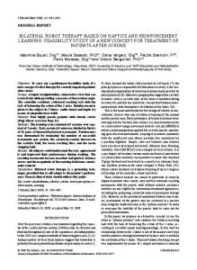
Figure 2.1: A Markov Decision Process. Large circles are states, small black dots are actions. Some states may have many actions. An action may lead to diering successor states with a given probability. For the RL framework we also add,  a reward function which, given a hs; a; s0 i triple generates a random scalar valued reward with a xed distribution. The reward for taking a in s and then entering s0 is a random variable whose expectation is de ned here as Rssa 0 . A process is said to be Markov if it has the Markov Property. Formally, the Markov Property holds if, P r(st+1 j st ; at ) = P r(st+1 j st ; at ; st 1 ; at 1 ; : : :): (2.1) holds. That is to say that the probability distribution over states entered at t + 1 is conditionally independent of the events prior to (st ; at ) { knowing the current state and action taken is suÆcient to de ne what happens at the next step. In reinforcement learning, we also assume the same for the reward function, P r(rt+1 j st ; at ) = P r(rt+1 j st ; at ; st 1 ; at 1 ; : : :): (2.2) The Markov property is a simplifying assumption which makes it possible to reason about optimality and proofs is a more straightforward way. For a more detailed account of MDPs see [21] or [114]. For the remainder of this section the terms process and environment will be used interchangeably under the assumption that the agent's environment can be exactly modelled as a discrete nite Markov process. In later chapters we examine cases where this assumption does not hold.

2.2 Policies, State Values and Return A policy, , determines how the agent selects actions from the state in which it nds itself. In general, a policy is any mapping from states to actions. A policy may be deterministic, in which case (st) = at, or it may specify a distribution over actions, (s; a) = P r(a = at js = st ). Once we have established a policy, we can ask how much return this policy generates from any given state in the process. Return is a measure of reward collected for taking a series of actions. The value of a state is a measure of expected return we can achieve for being in a state and following a given policy thereafter (i.e. its mean long-term utility). RL problems can therefore be further categorised by what estimate of return we want to maximise:

2.3.

9

POLICY EVALUATION

Here agents should act to maximise the immediate reward available from the current state. The value of a state, V (s), is de ned as, V  (s) = E [rt+1 j s = st ] (2.3) where E denotes an expectation given that actions are chosen according to . Finite Horizon Problems. Here agents should act to maximise the reward available given that there are just k more steps available to collect the reward. The value of a state is de ned as, ( 0; if k = 0,  V(k) (s) = E hrt+1 + V  (st+1 ) j s = st i ; otherwise. (2.4) (k 1)

Single Step Problems.

The agent should act to maximise the nite horizon return at each step (i.e. we act to maximise V(k) for all t, and k is a xed at every step). In nite Horizon Problems. The agent should act to maximise the reward available over an in nite future.

Receding Horizon Problems.

Most work in RL has centred around single-step and in nite horizon problems. In the in nite horizon case, it is common to use the total future discounted return as the value of a state: zt1 = rt + rt+1 +


+ k rt+1 +


(2.5) The parameter, 2 [0; 1], is a discount factor. Choosing < 1 denotes a preference to receiving immediate rewards to those in the more distant future. It also ensures that the return is bounded in cases where the agent may collect reward inde nitely (i.e. if the task is non-episodic or non-terminating), since all in nite geometric series have nite sums for a common ratio of, j j < 1. The in nite horizon case is also of special interest as it allows the value of a state to be concisely de ned recursively:   V  (s) = E zt1+1 j s = st = EX [rt+1 +X

V  (st+1 ) j s = st ] = (s; a) Pssa 0 Rssa 0 + V  (s0)
(2.6) a

s0

Equation 2.6 is known as a Bellman equation for V  (see [15]). Some environments may contain terminal states. Entering such a state means that no more reward can be collected this episode. To be consistent with the in nite horizon formalism, terminal states are usually modelled as a state in which all actions lead to itself and generate no reward. In practice, it is usually easiest to model all terminal states as a single special state, s+, whose value is zero and in which no actions are available. Terminal States

10

CHAPTER 2.

DYNAMIC PROGRAMMING

2.3 Policy Evaluation For some xed stochastic policy, , the iterative policy evaluation algorithm shown Figure 2.2 will nd an approximation of its state-value function, V^  (see also [114, 150]). The hat notation, x^, indicates an approximation of some true value, x. Step 5 of the algorithm simply applies the Bellman equation (2.6) upon an old estimate of V  to generate a new estimate (this is called a backup or update). Making updates for all states is called a sweep. It is intuitively easy to see that this algorithm will converge upon V  if 0  < 1. Assume that the initial value function estimate has a worst initial error of
0 in any state: V^0 (s) = V  (s) 
0 (2.7) Throughout,  is used to denote a bound in order to simplify notation. That is to say, V  (s)
0  V^0 (s)  V  (s) +
0 (2.8) and not,  ^V (s) = V  (s) +
0; or, (2.9) V (s)
0 : 1) Initialise V^0 with arbitrary nite values; k 0 2) do 3)
0 4) for each s 2 S P   P a 0 + V^ (s0 ) 5) V^k+1 (s) = a (s; a) s0 Pssa 0 Rss k 6)
max(
; jV^k+1(s) V^k (s)j ) 7) k k + 1 8) while
> T Figure 2.2: The synchronous iterative policy evaluation algorithm. Determines the value function of a xed stochastic policy to within a maximum deviation from V  of 1 T in any state for 0  < 1. 1) Initialise Q0 with arbitrary nite values; k 0 2) do 3)
0 4) for each hs; ai 2 SP A(s) a 0 + P 0  (s0 ; a0 )Q ^ k (s0; a0 ) 5) Q^ k+1 (s; a) = s0 Pssa 0 Rss a 6)
max(
; jQ^ k+1(s; a) Q^ k (s; a)j ) 7) k k + 1 8) while
> T Figure 2.3: The synchronous iterative policy evaluation algorithm for determining Q to  within 1 T .

2.3.

11

POLICY EVALUATION

After the rst iteration we have (at worst),   X X a 0 + V^ (s0 ) V^1 (s) = (s; a) Pssa 0 Rss 0 =

a

X

a

(s; a)

s0

X

s0

X

a 0 + (V  (s0 ) 
) Pssa 0 Rss 0




X

= 
0 + (s; a) Pssa 0 Rssa 0 + V  (s0)
a s0  = 
0 + V (s) (2.10) Note that only the true value-function, V  , and not its estimate, V^ , appears on the righthand side of 2.10. Continuing the iteration we have,   X X a 0 + V^ (s0 ) V^2 (s) = (s; a) Pssa 0 Rss 1 =

a

X

a

(s; a)

s0

X

s0

X

a 0 + (V  (s0 ) 
) Pssa 0 Rss 0




X

=  2
0 + (s; a) Pssa 0 Rssa 0 + V  (s0 )
a s0 2  = 
0 + V (s) ... V^k (s) =  k
0 + V  (s) (2.11) Thus if 0 < h < 1 ithen the convergence of V^ to V  is assured in the limit (as k ! 1) since limk!1 k
0 = 0. The following contraction mapping can be derived from 2.11 and states that each update strictly reduces the worst value estimate in any state by a factor of

(also see Appendix A) [114, 20, 17]: max jV^k+1(s) V  (s)j  max jV^k (s) V  (s)j: (2.12) s s The termination condition in step 8 of the algorithm allows it to stop once a satisfactory maximum error has been reached. This recursive process of iteratively re-estimating the value function in terms of itself is called bootstrapping. Since Equation 2.6 represents a system of linear equations, several alternative solution methods, such as Gaussian elimination, could be used to exactly nd V  (see [34, 80]). However, most of the learning methods described in this thesis are, in one way or another, derived from iterative policy evaluation and work by making iterative approximations of value estimates. 2.3.1 Q-Functions

In addition to state-values we can also de ne state-action values (Q-values) as: Q (s; a) = E [rt+1 + V  (st+1 )js =
st ; a = at ] X = Pssa 0 Rssa 0 + V  (s0) s0

(2.13)

12

CHAPTER 2.

DYNAMIC PROGRAMMING

Intuitively, this Q-function (due to Watkins, [163]) gives the value of following an action for one step plus the discounted expected value of following the policy thereafter. The expected value of a state under a given stochastic policy may be found solely from the Q-values at that state: V  (s)

=

X

a

(s; a)Q (s; a)

(2.14)

and so the Q-function may be fully de ned independently of V (by combining Equations 2.13 and 2.14): Q

(s; a) =

X

s0

Pssa 0

a0 Rss

+

X

a0

!

(s0 ; a0 )Q (s0 ; a0 )

(2.15)

It is straightforward to modify the iterative policy evaluation algorithm to approximate a Q-function instead of a state-value function (see Figure 2.3). Note that V and Q are easily interchangeable when given R and P . Also, from equation (2:14), it follows that knowing Q and  is enough to determine V (without R or P ). The reverse is not true. We will see in Section 2.4.2 that being able to compare action-values makes it trivial to make improvements to the policy. 2.3.2 In-Place and Asynchronous Updating

Step 5 of each algorithm in Figures 2.2 and 2.3 performs updates that have the form U^k+1 = f (U^k ), where U^ is a utility function, V^ or Q^ . That is to say, that a new value of every state or state-action pair is given entirely from the last value function or Q-function. The algorithms are usually presented in this way only to simplify proofs about their convergence. This form of updating is called synchronous or Jacobi-style [150]. A better method is to make the updates in-place [17, 150] (i.e. we perform U^ (s) f (U^ (s)) for one state, and make further backups to other states in the same sweep using this new estimate). This requires storing only one value function or Q function rather than two and is referred to as in-place or Gauss-Seidel updating. This method also usually converges faster since the values in the successor states upon which updates are based may have been updated within the same sweep and so are more up-to-date. A third alternative is asynchronous updating [20]. This is the same as the in-place method except it allows for states or state action pairs (SAPs) to be updated in any order and with varying frequency. This method is known to converge provided that all states (or SAPs) are updated in nitely often but with a nite frequency. An advantage of this approach is that the number of updates may be distributed unevenly, with more updates being given to more important parts of the state space [17, 18, 20].

2.4.

13

OPTIMAL CONTROL

2.4 Optimal Control In the previous section we have seen how to nd the long-term utility for being in a state, or being in a state and taking a speci c action, and then following a xed policy thereafter. While it's useful to know how good a policy is, we'd really prefer to know how to produce better policies. Ultimately, we'd like to nd optimal policies. 2.4.1 Optimality

An optimal policy,  , is any which achieves the maximum expected return when starting from any state in the process. The optimal Q-function, Q, is de ned by the Bellman optimality equation [15]: Q (s; a) = max Q (s; a)    X  (s0 ; a0 ) = Pssa 0 Rsa + max Q (2.16) a0 s0

Similarly, V  is given as: V  (s)

= max Q (s; a) a X a 0 Ra 0 + V  (s0 )
= max P ss ss a s0

(2.17)

There may be many optimal policies for some MDPs { this only requires that there are states whose actions yield equivalent expected returns. In such cases, there are also stochastic optimal policies for that process. However, every MDP always has at least one deterministic optimal policy. This follows simply from noting that if a SAP leads to a higher mean return than the other actions for that state, then it is better to always take that action than some mix of actions in that state. As a result most control optimisation methods seek only deterministic policies even though stochastic optimal policies may exist. 2.4.2 Policy Improvement

Improving a policy as a whole simply involves improving the policy in a single state. To do this, we make the policy greedy with respect to Q . The greedy action, ags , for a state is de ned as, ags = arg max Q(s; a) (2.18) a A greedy policy, g , is one which yields a greedy action in every state. An improved policy may be achieved by making it greedy in any state: (s) arg max Q(s; a) (2.19) a

14

CHAPTER 2.

1) k 0 2) do 3) nd Qk for k 4) for each s 2 S do 5) k+1 (s) = arg maxa Qk (s; a) 6) k k + 1 7) while k 6= k 1

DYNAMIC PROGRAMMING

Evaluate policy Improve policy

Figure 2.4: Policy Iteration. Upon termination  is optimal provided that Qk can be found accurately (see 2.4.3). In the improvement step (step 5), ties between equivalent action should be broken consistently to return a consistent policy for the same Q-function, and so also allow the algorithm to terminate. Step 3 is assumed to evaluate Q exactly. The policy improvement theorem rst stated by Bellman and Dreyfus [16] states that if,  (s; a)  X  (s; a)Q (s; a) max Q a a

holds then it is at least as good to take a greedy action in s than to follow  since, if the agent now passes through this state it can expect to collect at least maxa Q (s; a) (in the mean) P rather than a (s; a)Q (s; a) from there onward [16].1 The actual improvement may be greater since changing the policy at s may also improve the policy for states following from s in the case where s may be revisited during the same episode. The improved policy can be evaluated and then improved again. This process can be repeated until the policy can be improved no further in any state, at which point an optimal policy must have been found. The policy iteration algorithm shown in Figure 2.4 (adapted from [150], rst devised by Howard [56]) performs essentially this iterative process except that the policy improvement step is applied to every state in-between policy evaluations. Combinations of local improvements upon a xed Q will also produce strictly (globally) improving policies { any local improvement in the policy can only maintain or increase the expected return available from the states that lead into it. 2.4.3 The Convergence and Termination of Policy Iteration

Showing that the policy iteration algorithm terminates with an optimal policy in nite time is straightforward. Note that, i) the policy improvement step only produces deterministic policies, of which there are only jS jjAj and, ii) each new policy strictly improves upon the previous (unless the policy is already optimal). Put these facts together and it is clear that the algorithm must terminate with the optimal policy in less than nk improvement steps (k = jAj; n = jS j) [114]. In most cases this is a gross overestimate of the required number of iterations until termination. More recently, Mansour and Singh have provided a tighter bound of O( knn ) improvement steps [77]. Both of these bounds exclude the cost of evaluating the policy at each iteration. With Exact Q .

1

Implicitly, this statement rests on knowing Q accurately.

2.4.

15

OPTIMAL CONTROL

2

0 1 2 3 4 5

Vk (2) Vk (3) V0(2) V0 (3)

V0 (3) V0(2)

2 V0(2) 2 V0 (3)

3 V0 (3) 3V0 (2)

4 V0(2) 4 V0 (3)

. ..

3

4

5

1

3

1

k

2

. ..

k Vk (2) 0 1:000 1 0:900 2 0:810 3 0:590 4 0:531 5 0:387 6 0:349 7 0:254 8 0:229

Vk (3) Vk (4) Vk (5) 1:000 1:000 1:000 0:900 0:810 0:729 0:656 0:729 0:656 0:590 0:531 0:478 0:430 0:478 0:430 0:387 0:349 0:314 0:282 0:314 0:282 0:254 0:229 0:206 0:185 0:206 0:185

9 .. . .. . . .. . .. Figure 2.5: Example processes where the modi ed policy-iteration algorithm in Figure 2.4 converges to optimal estimates but fails to terminate if the evaluation of Q is approximate. In both processes, all rewards are zero and so V  (s) = Q(s; a) = 0 for all states and actions. Termination will not occur in each case because the greedy policy in the state 1 never stabilises. The actions in this state have equivalent values under the optimal policy but the greedy action ip- ops inde nitely between the two choices while there is any error in the value estimates. In both cases, the error is only eliminated as k ! 1 The value of the successor state selected by the policy in state 1 after policy improvement is shown in bold. (left) Synchronous updating with V0(2) > V0(3) > 0, and 0 < < 1. (right) In-place updating with = 0:9. Updates are made in the sequence given by the state numbers. The above proof requires that an accurate Q is found between iterations. Methods to do this are generally computationally expensive. An alternative method is modi ed policy iteration which employs the iterative (and approximate) policy evaluation algorithm from Section 2.3 to evaluate the policy in step 3 [114, 21]. Using the last found value or Q function as the initial estimate for the iterative policy evaluation algorithm will usually reduce the number of required sweeps required before termination. However, if Qk is only known approximately, then between iterations arg maxa Qk (s; a) may oscillate between actions for states where there are equivalent (or near-equivalent) true Q-values for the optimal policy.2 This can be true even if Qk monotonically continues to move towards Q since, in some cases, the Q-values of the actions in a state may improve at varying rates and so their relative order may continue to change. Figure 2.5 illustrates this new insight with two examples. With Approximate Q .

For practical implementations, it should be noted that due to the limitations of machine precision, even algorithms that are intended to solve Q precisely may suer from this phenomenon. 2

16

CHAPTER 2.

1) do: 2) V^ evaluate(, V^ ) 3)  0 4) for each s 2 S :   P a 0 + V^ (s0 ) 5) ag arg maxa s0 Pssa 0 Rss P ag ag ^ (s0 ) 6) v0 s0 Pss 0 Rss0 + V  7)  max ; V^ (s) v0 8) (s) ag Make  9) while   T

DYNAMIC PROGRAMMING

0 .

Figure 2.6: Modi ed Policy Iteration. Upon termination  is optimal to with some small error (see text). Overcoming this only requires that the main loop terminates when the improvement in the policy in any state has become suÆciently small (see the termination condition in Figure 2.6). The policy iteration algorithm published in [150] also requires the same change to guarantee its termination. The algorithm in Figure 2.6 guarantees that, 2 T V  (s)  V  (s) (2.20) 1 holds upon termination, for some termination threshold T . If T = 0 then the algorithm is equivalent to modi ed policy iteration. Part B of the Appendix establishes the straightforward proof of termination and error bounds { these follow directly from the work of Williams and Baird [172]. The proof assumes that the evaluate step of the revised algorithm applies,   X X a 0 + V^ (s0 ) V^ (s) (s; a) Pssa 0 Rss k s0

a

at least once for every state, either synchronously or asynchronously. 2.4.4 Value Iteration

The modi ed policy iteration algorithm alternates between evaluating Q^  for a xed  and then improving  based upon the new Q-function estimate. We can interleave these methods to a ner degree by using iterative policy evaluation to evaluate the greedy policy rather than a xed policy. This is done by replacing step 5 of the iterative policy evaluation algorithm in Figure 2.3 with:   X a 0 + max Q 0 0 ^ Pssa 0 Rss ( s ; a ) : (2.21) Q^ k+1 (s; a) k 0 s0

a

Note that, for the synchronous updating case, this new algorithm is exactly equivalent to performing 1 sweep of policy iteration followed by a policy improvement sweep { no policy

2.4.

17

OPTIMAL CONTROL

improvement step needs to be explicitly performed since the greedy policy is implicitly being evaluated by maxa0 Q^ k (s0; a0 ). It is less than obvious that this new algorithm will converge upon Q . As a policy evaluation method it is no longer evaluating a xed policy but chasing a non-stationary one. In fact the algorithm does converge upon Q as k ! 1. By considering the case where Q^ 0 = 0, we can see that (synchronous) value-iteration progressively solves a slightly dierent problem, and in the limit nds Q . Let a k-step nite horizon discounted return be de ned as follows: rt + rt+1 +


+ k 1 rk To behave optimally in a k-step problem is to act to maximise this return given that there are k-steps available to do so. Let (k)(s) denote an optimal policy for the k-step nite horizon problem. Then in the case where Q^ 0 = 0 we have, Q(1) (s; a) = E [rt+1 js = st ; a = at ] (2.22)   X = Pssa 0 Rssa 0 + max Q^ 0 (s; a) a0 s0

Thus after 1 sweep, the Q-function is the solution of the discounted 1-step nite horizon problem. That is to say, Q(1) predicts the maximum expected 1-step nite horizon return  (s) = arg maxa Q (s; a). and so (1) (1) Clearly, the optimal value of an action when there are 2 steps to go is the expected value of taking that action and then acting to maximise the discounted expected return with 1-step to go, 1-step on: h i Q(2) (s; a) = E rt+1 + E [rt+2 ] js = st ; a = at    (s; a0 )js = st ; a = at ; t+1 =  = E rt+1 + max Q (1) (1) a0 (1)

=

X

s0



a 0 + max Q (s; a0 ) Pssa 0 Rss (1) 0



a

 (s) = arg maxa Q (s; a) and is an optimal policy for the 2-step nite horizon Thus (2) (2) problem. With k steps to go we have:

Q(k+1) (s; a)

= = =

"

E rt+1 + E(k) 

" k X

i=2

#

i 1 rt+i js = st ; a = at

#

E rt+1 + max Q(k) (s; a0 )js = st ; a = at ; t+1 = (k) a0 X

s0

Pssa 0



a0 Rss



 0 + max 0 Q(k) (s; a ) a



(2.23)

So, under the assumption that the Q-function is initialised to zero, then it is clear that value-iteration (with synchronous updates) has solved the k-step nite horizon problem

18

CHAPTER 2.

DYNAMIC PROGRAMMING

after k iterations. That is to say that it nds the Q-function for the policy that maximises the expected k-step discounted return: h i k 1r max E r +

r +


+

(2.24) t t +1 k  which diers from maximising the expected in nite discounted return, h i k 1r +


max E r +

r +


+

(2.25) t t+1 k  by an arbitrary small amount for a large enough k and 0  < 1. Thus, value iteration assures that Q^ k converges upon Q as k ! 1 since Q^ (1) = Q , given Q^ 0(s; a) = 0 and 0  < 1. A more rigorous proof that applies for arbitrary ( nite) initial value functions was established by Bellman [15] and can be found in Section A.4. In particular, the following contraction mapping can be shown which avoids the need to assume Q^ 0 = 0, max jV^k+1(s) V (s)j  max jV^k (s) V (s)j: (2.26) s s Proofs of convergence for the in-place and asynchronous updating case have also been established [17].

2.5 Summary We have seen how dynamic programming methods can be used to evaluate the long-term utility of xed policies, and how, by making the evaluation policy greedy, optimal policies may also be converged upon. Value iteration and policy iteration form the basis of all of the RL algorithms detailed in this thesis. Although they are a powerful and general tool for solving diÆcult multi-step decision problems in stochastic environments, the MDP formalism and dynamic programming methods so far presented suer a number of limitations: 1. Availability of a Model Dynamic Programming methods assume that a model of the environment (P and R) is available in advance, and that no further knowledge of, or

interaction with, the environment is required in order to determine how to act optimally within it. However, in many cases of interest, a prior model is not generally available, nor is it always clear how such a model might be constructed in any eÆcient manner. Fortunately, even without a model, a number of alternatives are available to us. It remains possible to learn a model, or even learn a value function or Q-function directly through experience gained from within the environment. Reinforcement learning through interacting with the environment is the subject of the next chapter. In many practical problems, a state might correspond to a point in a high dimensional space: s = hx1; x2 ; : : : ; xni. Each dimension corresponds to a particular feature of the problem being solved. For instance, suppose our task is to design 2. Small Finite Spaces

2.5.

SUMMARY

19

an optimal strategy for the game of tic-tac-toe. Each component of the board state, xi, describes the position of one cell in a 3  3 grid (1  i  9), and can take one of three values (\X", \O" or \empty"). In this case, the size of the state space is 39 . For a game of draughts, we have 32 usable tiles and a state space size of the order of 332 . In general, given n features each of which can take k possible values, we have a state space of size kn . In other words, the size of the state space grows exponentially with its dimensionality. Correspondingly, so grows the memory required to store a value function and the time required to solve such a problem. This exponential growth in the space and time costs for a small increase in the problem size is referred to as the \Curse of Dimensionality" (due to Bellman, [15]). Similarly, if the state-space has in nitely many states (e.g. if the state-space is continuous) then it is simply impossible to exactly store individual values for each state. In both cases, using a function approximator to represent approximations of the value function or model can help. These are discussed in Chapter 6. 3. Markov Property In practice, the Markov property is hard to obtain. There are many cases where the description of the current state may lack important information necessary to choose the best action. For instance, suppose that you nd yourself in a large building where many of the corridors look the same. In this case, based upon what is seen locally, it may be impossible to decide upon the best direction to move given that some other part of the building looks the same but where some other direction is best. In many instances such as this, the environment may really be an MDP, although it may not be the case that the agent can exactly observe its true state. However, the prior sequence of observations (of states, actions, rewards and successors) often reveal useful information about the likely real state of the process (e.g. if I remember how many ights of stairs I went up I can now tell which corridor I am in with greater certainty). This kind of problem can be formalised as a Partially Observable Markov Decision Process (POMDP). A POMDP, is often de ned as an MDP, which includes S , A, P and a reward function, plus a set of prior observations and a mapping from real states to observations. These problems and their related solution methods are not examined in this thesis. See [27] or [74] for excellent introductions and eld overviews.

The MDP formalism assumes that there is a xed, discrete amount of time between state observations. In many problems this is untrue and events occur at varying real-valued time intervals (or even occur continuously). A good example is the state of a queue for an elevator [36]. At t = 0 the state of the queue might be empty (s0). Some time later someone may join the queue (we make a transition to s1), but the time interval between states transitions can take some real value whose probability may be given by a continuous distribution. Variable and continuous time interval variants of MDPs are referred to as a Semi-Markov Decision Process (SMDPs) [114], and are examined in Chapter 7. 4. Discrete Time

20

CHAPTER 2.

DYNAMIC PROGRAMMING

In cases where reward may be collected inde nitely and discounting is not desired, the discounted return model may not be used since the future sum of rewards with = 1 may be unbounded. Furthermore, even in cases where the returns can be shown to be bounded, with = 1 the policy-iteration and value-iteration algorithms are not guaranteed to converge upon Q. This follows as a result of using bootstrapping and the max operator which causes any optimistic initial bias in the Q-function to remain inde nitely. If discounting is not desired, then an average reward per step formalism can be used. Here the expected return is de ned as follows [132, 153, 75, 21]: n 1X E [rt js = st ]  = lim 5. Undiscounted Ergodic Tasks

n!1 n

t=1

This formalism is problematic in processes where all states are reachable from any other under the policy (such as process is said to be ergodic). However, even in this case, from some states higher than average return may be gained for some short time and so such a state might be considered to be better. Quantitatively, the value of a state can be de ned by the relative dierence between the long-term average reward from any state,  , and the reward following a starting state: V (s)

=

1 X

k=1

E [rt+k

 jst = s; ]

Thus a policy may be improved by modifying it to increase the time that the system spends in high valued states (thereby raising ). Average reward methods are not examined in this thesis.

Chapter 3

Learning from Interaction Chapter Outline

In this chapter we see how reinforcement learning problems can be solved solely through interacting with the environment and learning from what is observed. No knowledge of the task being solved needs to be provided. A number of standard algorithms for learning in this way are reviewed. The shortcomings of exploration insensitive model-free control methods are highlighted, and new intuitions about the online behaviour of accumulate trace TD() methods illustrated.

3.1 Introduction The methods in the previous chapter showed how to nd optimal solutions to multi-step decision problems. While these techniques are invaluable tools for operations research and planning, it is diÆcult to think of them as techniques for learning. No experience is gathered { all of the necessary information required to solve their task of nding an optimal policy is known from the outset. The methods presented in this chapter start with no model (i.e. P and R are unknown). Every improvement made follows only from the information collected through interactions with the environment. Most of the methods follow the algorithm pattern shown in Figure 3.1. Broadly, (value-based) RL methods for learning through interaction can be split into two categories. Indirect methods use their experiences in the environment to construct a model of it, usually by building estimates of the transition and reward functions, P and R. This model can then be used to generate value-functions or Q-functions using, for instance, methods similar to the dynamic 21 Direct and Indirect Reinforcement Learning

22

CHAPTER 3.

LEARNING FROM INTERACTION

1) for each episode: 2) Initialise: t 0; st=0 3) while st is not terminal: 4) select at 5) follow at ; observe, rt+1, st+1 6) perform updates to P^ , R^ , Q^ and/or V^ using the new experience hst ; at ; rt+1 , st+1i 7) t t+1 Figure 3.1: An abstract incremental online reinforcement learning algorithm. programming techniques introduced in the last chapter. Indirect methods are also termed model-based (or model-learning) RL methods. Alternatively, we can learn value-functions and Q-functions directly from the reward signal, forgoing a model. This is called the direct or model-free approach to reinforcement learning. This chapter rst presents an incremental estimation rule. From this we see how the direct methods are derived and then the indirect methods.

3.2 Incremental Estimation of Means Direct methods can be thought of as algorithms that attempt to estimate the mean of a return signal solely from observations of that return signal. For most direct methods, this is usually done incrementally by applying an update rule of the following form: Z^k = RunningAverage(Z^k 1 ; zk ; k ) = Z^k 1 + k (zk Z^k 1) (3.1) where Z^k is the new estimated mean which includes the kth observation, zk , of a random variable, and k 2 [0; 1] is a step-size (or learning rate) parameter. Each observation is assumed to be a bounded scalar value given a random variable with a stationary distribution. By de ning the learning rate in dierent ways the update rule can be given a number of useful properties. These are listed below. Running Average. With k observations fz1 ; : : : ; zk g,

= 1=k, Z^k is the sample mean (i.e. average) of the set of Z^k =

k 1X zi

k i=1

The following derivation of update 3.1 is from [150], +1 1 kX Z^k+1 = z k + 1 i=1 i

(3.2)

3.2.

23

INCREMENTAL ESTIMATION OF MEANS

= = = = =

!

k 1 z +X z k + 1 k+1 i=1 i k !! 1 z +k 1 X z k + 1 k+1 k i=1 i 1 z + kZ^  k k + 1 k+1  1 z + (k + 1)Z^ Z^  k k k + 1 k+1  1 z Z^k + k+1 Z^k k+1

(3.3)

By choosing a constant value for , (where 0 <  < 1), update 3.1 can be used to calculate a recency weighted average. This can be seen more clearly by expanding the right hand side of Equation 3.1: Z^t+1 = zt+1 + (1 )Z^t (3.4) Intuitively, each new observation forms a xed percentage of the new estimate. Recency weighted averages are useful if the observations are drawn from a non-stationary distribution. In cases where 1 6= 1 the estimates Z^k (k > 1) may be partially determined by the initial estimate, Z^0. Such estimates are said to be biased by the initial estimate. Z^0 is an initial bias. Recency Weighted Average.

Mean in the Limit.

have,

From standard statistics, with k = 1=k, from Equation 3.2 we

lim Z^k = E [z]: However, more usefully, Equation 3.5 also holds if, k!1

1) 2)

1 X

k=1

1 X

k=1

(3.5)

k = 1

(3.6)

2k < 1;

(3.7)

both hold. These are the Robbins-Monro conditions and appear frequently as conditions for convergence of many stochastic approximation algorithms [126]. The rst condition ensures that, at any point, the sum of the remaining stepsizes is in nite and so the current estimate will eventually become insigni cant. Thus, if the current estimate contains some kind of bias, then this is eventually eliminated. The second condition ensures that the step sizes eventually become small enough so that any variance in the observations can be overcome. In most interesting learning problems, there is the possibility of trading lower bias for higher variance, or vice versa. Slowly declining learning rates reduce bias more quickly but

24

CHAPTER 3.

LEARNING FROM INTERACTION

converge more slowly. Reducing the learning rate quickly gives fast convergence but slow reductions in bias. If the learning rate is declined too quickly, premature convergence upon a value other than E [z] may occur. The Robbins-Monro conditions guarantee that this cannot happen. Conditions 1 and 2 are known to hold for, 1 ; k (s) = (3.8) k(s) at the kth update of Z^(s) and 1=2 <  1 [167].

3.3 Monte Carlo Methods for Policy Evaluation This section examines two model-free methods for performing policy evaluation. That is to say, given an evaluation policy, , they obtain the value-function or Q-function that predicts the expected return available under this policy without the use of an environmental model. Monte Carlo estimation represents the most basic value prediction method. The idea behind it is simply to nd the sample mean of the complete actual return, zt1 = rt+1 + rt+2 +


for following the evaluation policy after a state, or SAP (state-action pair), until the end of the episode at time T . The evaluation policy is assumed to be xed and is assumed to be followed while collecting these rewards. If a terminal state is reached then, without loss of generality, the in nite sum can be truncated by rede ning it as, zt1 = rt+1 + rt+2 +


+ T 1 rT + T V (sT ) where V (sT ) is the value of the terminal state sT . Typically, this is de ned to be zero. Again this is without loss of generality, since rT can be rede ned to re ect the diering rewards for entering dierent terminal states. Singh and Sutton dierentiate between two avours of Monte Carlo estimate { these are the rst-visit and every-visit estimates [139]. The every-visit Monte Carlo estimate is de ned as the sample average of the observed return following every visit to a state: M 1X z1 (3.9) V^E (s) = Every Visit Monte Carlo Estimation.

M i=1

ti

where s is visited at times ft1 ; : : : tM g. In this case, the RunningAverage update is applied oine, at the end of each episode at the earliest. Each state-value is updated once for each state visit using the return following that visit. M represents the total number of visits to s in all episodes.

3.3.

MONTE CARLO METHODS FOR POLICY EVALUATION

25

Ps ; Rs s

PT ; RT

T

Figure 3.2: A simple Markov process for which rst-visit and every-visit Monte Carlo approximation initially nd dierent value estimates. The process has a starting state, s, and a terminal state, T . Ps and PT denote the respective transition probabilities for s ; s and for s ; T . The respective rewards for these transitions are Rs and RT . The rst-visit Monte Carlo estimate is de ned as the sample average of returns following the rst visit to a state during the episodes in which it was visited: N 1X V^F (s) = zt1i (3.10) First Visit Monte Carlo Estimation.

N i=1 times ft1; : : : ; tN g and N

where s is rst visited during an episode at represents the total number of episodes. The key dierence here is that an observed reward may be used to update a state value only once, whereas in the every-visit case, a state value may be de ned as the average of several non-independent return estimates, each involving the same reward, if the state is revisited during an episode. In the case where state revisits are allowed within a trial these methods produce dierent estimators of return. Singh and Sutton analysed these dierences which can be characterised by considering the process in Figure 3.2 [139]. For simplicity assume = 1, then from the Bellman equation (2.6) the true value for this process is: V (s) = Ps (Rs + V (s)) + PT RT (3.11) = PsR1s + PPT RT (3.12) Bias and Variance.

=

s

Ps R + RT PT s

(3.13)

Consider the dierence between the methods following one episode with the following experience, s;s;s;s;T

The rst-visit estimate is:

V^F (s) = Rs + Rs + Rs + RT

while the every-visit estimate is: R + 2Rs + 3Rs + 4RT V^E (s) = s 4

26

CHAPTER 3.

LEARNING FROM INTERACTION

For both cases, it is possible to nd the expectation of the estimate after one trial for some arbitrary experience. This is done by averaging the possible returns that could be observed in the rst episode weighted their probability of being observed. For the rst-visit case, it can be shown that after the rst episode [139], h i P E V^1F (s) = s Rs + RT PT = V (s) and so is an unbiased estimator of V (s). After N episodes, V^NF (s) is the sample average of N independent unbiased estimates of V (s), and so is also unbiased. For the every-visit case, it can be shown (in [139]) that after the rst episode, h i Ps E V^1E (s) = 2PT Rs + RT where k denotes the number of times that s is visited within the episode. Thus after the rst episode the every-visit method does not give an unbiased estimate of V (s). Its bias is given by, h i BIASE1 = V (s) E V^1E (s) = 2PPs Rs: (3.14) T Singh and Sutton also show that after M episodes, (3.15) BIASEM = M 2+ 1 BIASE1 : Thus the every-visit method is also unbiased as M ! 1. The bias in the every-visit method comes from the fact that it uses some rewards several times. Thus many of the return observations are not independent. However, the observations between trials are independent, and so as the number of trials grows, its bias shrinks. Both methods converge upon V (s) as M or N tend to in nity. Singh and Sutton also analysed the expected variance in the estimates learned by each method. They found that, while the rst-visit method has no bias, it initially has a higher expected variance than the every-visit method. However, its expected variance declines far more rapidly, and is usually lower than for the every-visit method after a very small number of trials. Thus, in the long-run the rst-visit method appears to be superior, having no bias and lower variance.

3.4 Temporal Dierence Learning for Policy Evaluation 3.4.1 Truncated Corrected Return Estimates

Because the return estimate used by the Monte Carlo method (i.e. the observed return, z (1) ) looks ahead at the rewards received until the end of the episode, it is impossible to make updates to the value function based upon it during an episode. Updates must be

3.4.

TEMPORAL DIFFERENCE LEARNING FOR POLICY EVALUATION

27

made in between episodes. If the task is non-episodic (e.g. if the environment never enters a terminal state), it seems unlikely that a Monte Carlo method can be used at all. One possibility is to make the task episodic by breaking the episodes into stages. The stages could be separated by a xed number of steps, by replacing z (1) = rt+1 + rt+2 +


+ n 1 rt+n +


with, z (n) = rt+1 + rt+2 +


+ n 1 rt+n + n U (st+n ) where U (st+n) is a return correction and predicts the expected return for following the evaluation policy from st+n. Note that this is already done to deal with terminal states in the Monte-Carlo method. However, if st+n is not a terminal state we typically will not know the true utility of st+n under the evaluation policy. Instead we replace it with an estimate { the current V^ (st+n) for example. The next section introduces a special case where n = 1. Updates are performed after each and every step using knowledge only about the immediate reward collected and the next state entered. 3.4.2 TD(0)

The temporal dierence learning algorithm, TD(0), can be used to evaluate a policy and works through applying the following update [13, 147, 148]:   V^ (st ) V^ (st ) + t (st ) rt+1 + V^ (st+1 ) V^ (st ) ; (3.16) where rt+1 is the reward following at taken from st and selected according the policy under evaluation. Note that this has the same form as the RunningAverage update rule where the target is E [rt+1 + V^ (st+1 )]. Recall from Equation 2.6 that,   X X a 0 + V^ (s0 ) V^ (s) = (s; a) Pssa 0 Rss a s0 h i = E rt+1 + V^ (st+1 )js = st;  So, assuming for the moment that V^ (st+1 ) is a xed constant, Update 3.16 can be seen as a stochastic version of,   X X a 0 + V^ (s0 ) ; V^ (s) (s; a) Pssa 0 Rss (3.17) a

s0

h i where E rt+1 + V^ (st+1 )js = st ;  is estimated in by V^ (s) in the limit from the observed (sample) return estimates, rt+1 + V^t (st+1), rather than the target return estimate given by the right-hand-side of update 3.17. TD(0) is reliant upon observing the return estimate, r + V^ (s0), and applying it in update 3.16 with the probability distribution de ned by R, P and . This can be done in several

28

CHAPTER 3.

LEARNING FROM INTERACTION

1) for each episode: 2) initialise st 3) while st is not terminal: 4) select at according to  5) follow at ; observe, rt+1, st+1 6) TD(0)-update(st , at , rt+1, st+1) 7) t t+1 TD(0)-update(st, at , rt+1 , st+1  )  1) V (st) V^ (st ) + t+1 (st ) rt+1 + V^ (st ) V^ (st)

Figure 3.3: The online TD(0) learning algorithm. Evaluates the value-function for the policy followed while gathering experience. ways, but by far the most straightforward is to actually follow the evaluation policy in the environment and make updates after each step using the experience collected. Figure 3.3 shows this online learning version of TD(0) in full. Note that it makes no use of R or P . In general, the value of the correction term (V^ (st+1) in update 3.16) is not a constant but is changing as st+1 is visited and its value updated. The method can be seen to be averaging return estimates sampled from a non-stationary distribution. The return estimate is also biased by the initial value function estimate, V^0. Even so, the algorithm can be shown to converge upon V  asP1t ! 1 providedPthat the learning rate is declined under the Robbins1 Monro conditions ( k=1 k (s) = 1; k=1 2k (s; a) < 1), that all value estimates continue to be updated, the process is Markov, all rewards have nite variance, 0  < 1 and that the evaluation policy is followed [148, 38, 158, 59, 21]. In practice it is common to use the xed learning rate  = 1 if the transitions and rewards are deterministic, or some lower value if they are stochastic. Fixed  also allows continuing adaptation in cases where the reward or transition probability distributions are non-stationary (in which case the Markov property does not hold). 3.4.3 SARSA(0)

Similar to TD(0), SARSA(0) evaluates the Q-function of an evaluation policy [128, 173]. Its update rule is: Q^ (st ; at )

Q^ (st ; at ) + k rt+1 + Q^ (st+1 ; at+1 ) Q^ (st ; at ) ; 



(3.18)

where at and at+1 are selected with the probability speci ed by the evaluation policy and k = k (st ; at ). SARSA diers from the standard algorithm pattern given in Figure 3.1 because it needs to know the next action that will to be taken when making the value update. The SARSA algorithm is shown in Figure 3.4. An alternative scheme that appears to be equally valid and is more closely related to the policy-evaluation Q-function update (see Equation 2.15

3.4.

TEMPORAL DIFFERENCE LEARNING FOR POLICY EVALUATION

29

1) for each episode: 2) initialise st 3) select at according to  4) while st is not terminal: 5) follow at; observe, rt+1 , st+1 6) select at+1 according to  7) SARSA(0)-update(st , at , rt+1 , st+1, at+1 ) 8) t t+1 SARSA(0)-update(st , at, rt+1, st+1 , at+1)  1) Q^ (st ; at ) Q^ (st ; at ) + k rt+1 + Q^ (st+1 ; at+1 ) Q^ (st ; at )

Figure 3.4: The online SARSA(0) learning algorithm. Evaluates the Q-function for the policy followed while gathering experience. and Figure 2.3) is to replace the target return estimate with [128]: X rt+1 + (st+1 ; a0 )Q^ (st+1 ; a0 ): a0

(3.19)

An algorithm employing this return does not need to know at+1 to make the update and so can be implemented in the standard framework. Its independence of at+1 also makes this an o-policy method { it doesn't need to actually follow the evaluation policy in order to evaluate it. This property is discussed in more detail later in this chapter. However, unlike regular SARSA, this method does require that the evaluation policy is known, which may not always be the case { experience could be generated be observing an external (e.g. human) controller. 3.4.4 Return Estimate Length Single-Step Return Estimates

The TD(0) and SARSA(0) algorithms are single-step temporal dierence learning methods and apply updates to estimate some target return estimate having the following form: zt(1) = rt + U^ (st ); (3.20) It is important to note that it is the dependence upon using only information gained from the immediate reward and the successor state that allows single-step methods to be easily used as an online learning algorithms. However, when single-step learning methods are applied in the standard way, by updating V^ (st ) or Q^ (st ; at ) at time t + 1, new return information is propagated back only to the previous state. This can result in extremely slow learning in cases where credit for visiting a particular state or taking a particular action is delayed by many time steps. Figure 3.5 provides an example of this problem. Each episode begins in the leftmost state. Each state to the right is visited in sequence until the rightmost (terminal) state is entered where a reward of 1 is given (r = 0 in all other states). In such a situation, it would take 1-step methods a minimum of 64 episodes before any information

30

CHAPTER 3.

t= 0

...

LEARNING FROM INTERACTION

t= 6 3

t= 6 4 r= 1

Figure 3.5: The corridor task. Single-step updating methods such as TD(0), SARSA(0) and Q-learning can be very slow to propagate any information about the terminal reward to the leftmost state. about the terminal reward reaches the leftmost state. A Monte Carlo estimate would nd the correct solution after just one episode. Multi-Step Return Estimates

By modifying the return estimate to look further ahead than the next state, a single experience can be used to update utility estimates at many previously visited states. For example, the 1-step return in 3.16, zt(1) = rt + U (st), may be replaced with the corrected n-step truncated return estimate, zt(n) = rt + rt+1 +


+ n 1 U^ (st+n ) (3.21) or we may use, h i zt = (1 ) zt(1) + zt(2) + 2 zt(3) +


(3.22)     = (1 ) rt + U^ (st+1 ) +  rt + zt+1 (3.23) = rt + (1 ) U^ (st+1 ) +  zt+1 (3.24) which is a -return estimate [147, 148, 163, 128, 107]. The -return estimate is important as it is a generalisation of both z(1) and z(1) since, if  = 0, then z = z(1) , and if  = 1, then z = z(1) , or the actual discounted return. A key feature of multi-step estimates is that a single observed reward may be used in updating the state-values or Q-values in many previously visited states. Intuitively, this oers the ability to more quickly assign credit for delayed rewards. The return estimate length can also be seen as managing a tradeo between bias and variance in the return estimate [163]. When  is low, the estimate is highly biased toward the initial state-value or Q-function. When  is high the estimate involves mainly the actual observed reward and is a less biased estimator. However, unbiased return estimates don't necessarily result in the fastest learning. Typically, longer return estimates have higher variance as there is a greater space of possible values that a multi-step return estimate could take. By contrast, a single-step estimate is limited to taking values formed by combinations of the possible immediate rewards and the values of immediate successor states, and so may typically have lower variance. Also, employing the already-learned value estimates of successor states in updates may also help speed up learning since these values may contain summaries of the complex future that may follow from the state. Best performance is often to be found with intermediate values of  [148, 128, 73, 139, 150].

3.4.

TEMPORAL DIFFERENCE LEARNING FOR POLICY EVALUATION

31

However, while multi-step estimates appear to oer faster delayed credit assignment they seem to suer the same problem as the Monte-Carlo methods { that the updates must either be made o-line, at the end of each episode, or that episodes are split into stages and the return estimates truncated. Chapter 4 introduces a method which explores the latter case. The next section shows how the eect of using the -return estimate can be approximated by a fully incremental online method that makes updates after each step. 3.4.5 Eligibility Traces: TD()

This section shows how -return estimates can be applied as an incremental online learning algorithm. This is surprising because it implies that it is not necessary to wait until all the information used by the -return estimate is collected before a backup can be made to a previously visited state. The eect of using z can be closely and incrementally approximated online using eligibility traces [148, 163]. A -return algorithm performs the following update,   V^ (st ) V^ (st ) + t (st ) zt+1 V^ (st ) : (3.25) By Equation 3.24 Sutton showed that the error estimate in this update can be re-written as [148, 163, 107], zt+1 V^ (st ) = Æt + Æt+1 + : : : + ( )k Æt+k + : : : (3.26) where Æt is the 1-step temporal dierence error as before, Æt = rt+1 + V^ (st+1 ) V^ (st ): If the process is acyclic and nite (and so necessarily also has a terminal state), this allows update 3.25 to be re-written as the following on-line update rule, which overcomes the need to have advance knowledge of the 1-step errors, V^ (s)

V^ (s) + t (s)Æt

t X k=t0

( )t k I (s; sk)

(3.27)

where t0 indicates the time of the start of the episode, and I (s; sk ) is 1 if s was visited at t k, and zero otherwise. This update must be applied to all states visited at time t or before, within the episode. In the case in which state revisits may occur, the updates may be postponed and a single batch update may be made for each state at the end of the episode, V^ (s)

V^ (s) +

where sT is the terminal state.

TX1 t=t0

t (s)Æt

t X

( )t k I (s; sk )

k=0

32

CHAPTER 3.

LEARNING FROM INTERACTION

TD()-update(st, at, rt+1 , st+1 ) 1) Æ rt+1 + V^ (st+1 ) V^ (st) 2) e(s) e(s) + 1 3) for each s 2 S : 3a) V^ (s) V^ (s) + e(s)Æ 3b) e(s) e(s)

Figure 3.6: The accumulating-trace TD() update. This update step should replace TD(0)update in Figure 3.3 for the full learning algorithm. All eligibilities should be set to zero at the start of each episode. However, the above methods don't appear to be of any extra practical use than the MonteCarlo or -return methods. If the task is acyclic, then then there is little bene t for having an online learning algorithm since the agent cannot make use of the values it updates until the end of the episode. So the assumption preventing state revisits is often relaxed. In this case the error terms may be inexact since the state-values used as the return correction may have been altered if the state was previously visited. However, intuitively this seems to be a good thing since the return correction is more up-to-date as a result. To avoid the expensive recalculation of the summation in 3.27, this term can be rede ned as, V^ (s)

V^ (s) + t et (s)Æt

(3.28)

where e(s) is an (accumulating) eligibility trace. For each state at each step it is updated as follows, et (s)

=



et 1 (s) + 1;

et 1 (s);

if s = st, otherwise.

(3.29)

The full online TD() algorithm is shown in Figure 3.6. Both the online and batch TD() algorithms are known to converge upon the true state-value function for the evaluation policy under the same conditions as TD(0) [38, 158, 59, 21]. The intuitive idea behind an eligibility trace is to make a state eligible for learning for several steps after it was visited. If an unexpectedly good or bad event happens (as measured by the temporal dierence error, Æ), then all of the previously visited states are immediately credited with this. The size of the value adjustment is scaled by the state's eligibility, which decays with the time since the last visit. Moreover, the 1-step error Æt measures an error in the -return used, not just for the previous state, but for all previously visited states in the episode. The eligibility measures the relevance of that error to the values of the previous states given that they were updated using a -return corrected for the error found at the current state. Thus it should be clear why the trace decays as ( )k { the contribution of V^ (st+k ) to zt() is ( )k .

3.4.

TEMPORAL DIFFERENCE LEARNING FOR POLICY EVALUATION

33

The Forward-Backward Equivalence of Batch TD() and -Return Updates

If the changes to the value-function that the accumulate-trace algorithm is to make during an episode, are summed, TX1
V (s) = t et (st )Æt t=0

and applied at the end of the episode (instead of online), V (s) V (s) +
V (s) it can be shown that this is equivalent to applying the -return update,   V^ (s) V^ (s) +  zt+1 V^ (s) ; at the end of the episode, for each s = st visited during the episode [150].1 Thus in the case where  = 1, and k (s) = 1=k(s), this batch mode TD() method is equivalent to the every-visit Monte Carlo algorithm. The proof of this can be found in [139] and [150]. Below, the direct -return method is referred to a the forward-view, and the eligibility trace method as the backward-view (after [150]). 3.4.6 SARSA()

The equivalent version of TD() for updating a Q-function is SARSA(), shown in Figure 3.7 [128, 129]. Here, an eligibility value is maintained for each state-action pair. SARSA()-update(st, at , rt+1, st+1 , at+1 ) 1) Æ rt+1 + Q^ (st+1; at+1 ) Q^ (st; at ) 2) e(s; a) e(s; a) + 1 3) for each s 2 S 3a) Q^ (s; a) Q^ (s; a) + e(s; a)Æ 3b) e(s; a) e(s; a)

Figure 3.7: The accumulating-trace SARSA() update. This update step should replace the SARSA(0)-update in Figure 3.4 for the full learning algorithm. All eligibilities should be set to zero at the start of each episode. 3.4.7 Replace Trace Methods

In practice, accumulating trace methods are known to often work poorly, especially with  close to 1 [139, 149, 150]. In part, this is likely to be the result of its relationship with the See also the special case of the forwards-backwards equivalence proof in Appendix C where  = 1. This proof is a generalisation of the one in [150]. 1

34

CHAPTER 3.

LEARNING FROM INTERACTION

every-visit Monte-Carlo algorithm. An alternative eligibility trace scheme is the replacing trace:  1; if s = st, et (s) = e (s); otherwise. (3.30) t 1 Sutton refers to this as a recency heuristic { the eligibility of a state depends only upon the time since the last visit. By contrast, the accumulating trace is a frequency and recency heuristic. In [139] Sutton and Singh show that, with  = 1 and with appropriately declining learning rates, the batch-update TD() algorithms exactly implement the Monte Carlo algorithms. In particular, it can be shown that accumulating traces give the every-visit method, and replacing traces give the rst-visit Monte Carlo method. In addition to the better theoretical bene ts of every-visit Monte Carlo, the replace trace method has often performed better in online learning tasks. In [150] Sutton and Barto also prove that the TD() and forward-view -return methods are identical in the case of batch (i.e. oine) updating for general  with a constant . When estimating Q-values two replace-trace schemes exist. These are the state-replacing trace [139, 150], 8 if s = st and a = at , < 1; 0 ; if s = st and a 6= at , et (s; a) = : (3.31)

et 1 (s; a); if s 6= st . and the state-action replacing trace [33],  1; if s = st and a = at , et (s; a) = e (s; a); otherwise. (3.32) t 1 3.4.8 Acyclic Environments

If the environment is acyclic, then the dierent eligibility updates produce identical eligibility values and so the accumulate and replace trace methods must be identical. In this case, the online and batch versions of the algorithms are also identical since the return corrections used in return estimates must be xed within an episode. With  = 1, the -return methods also implement the Monte Carlo methods in acyclic environments. Also, here, both rst-visit and every-visit methods are equivalent. The eligibility trace methods appear to be considerably more expensive than the other model-free methods so far presented. For TD(0) and SARSA(0) the time-cost per experience is O(1). The Monte-Carlo and direct -return methods have the same cost if the returns are calculated starting with the most recent experience and working backwards.2 Algorithms working in this way will be seen in Chapter 4. By contrast, TD() has a time-cost as high as O(jS j) per experience. Thus the great bene t aorded by using eligibility traces is that they allow multi-step return estimates to be used for continual online learning and, as a consequence, can also be used in Since all discounted return estimators can be calculated recursively as, zt = f (rt ; st ; at ; zt+1 ; U ); for some function f . If zt+1 is known then it is cheap to calculate zt by working backwards. 2

3.4.

TEMPORAL DIFFERENCE LEARNING FOR POLICY EVALUATION

Æt Zt

Æt

Zt+1

35

Æt

zt

Figure 3.8: Number line showing eect of step-size. Note that having a step-size greater 2 can actually increase the error in the estimate (i.e. moving the new estimate into the hashed area). non-episodic tasks and in cyclical environments in a relatively straightforward way. We will see in the next chapter that the cost of the eligibility trace updates can be greatly reduced. 3.4.9 The Non-Equivalence of Online Methods in Cyclic Environments

Consider the RunningAverage update rule (3.1). It is easy to see that with a large learning rate the algorithm can actually increase the error in the prediction. Let Æt = zt Z^t 1, then if  > 2 and after an update, jzt Z^t+1j > jzt Z^t j. The problem can be seen visually in Figure 3.8. This raises new suspicions about the online behaviour of the accumulate trace TD() update. In a worst case environment (see Figure 3.9) in which a state is revisited after every step, after k revisits the eligibility trace becomes, ek (s) = 1 +  +


+ ( )k 1 )k = 1 1 ( 



Thus, for  < 1, an upper bound on an accumulating eligibility trace (in any process) is given by, 1 (3.33) e1 (s) = 1  For  = 1 the trace grows without bound if the process is nite and has no terminal state. The TD() update (3.28) makes updates of the following form: V (s) V (s) + t (s)et (s)Æ: Thus it might seem that where t (s)et (s) > 2 holds the TD() algorithm could grow in error with each update. These conditions are easily satis ed for  close enough to 1 in any non-terminating nite (and therefore cyclic) process. Considering the case where the trace reaches its upper bound, we have in the worst case scenario, 1 > 2 t (s) 1 

36

CHAPTER 3.

LEARNING FROM INTERACTION

t et

20

15

10

s 5

Figure 3.9: A worst-case environment for accumulating eligibility trace methods where the state's eligibility grows at the maximum rate. The reward is a random variable chosen from the range [ 1; 1] with a uniform distribution.

0 1

10

100 Time, t

1000

10000

Figure 3.10: The growth of the accumulate trace update step-size for the process in Figure 3.9. The learning rate is t = t 1: , = 0:999 and  = 1:0. These settings satisfy the conditions of convergence for accumulate trace TD(). 0 55

1 t2(s) <  assuming a constant t (s) while the eligibility rises. Yet the convergence of online accumulate trace TD() has already been established [38, 59]. Crucially these rely upon the learning rate being declined under the Robbins-Monro conditions which ensures that  tends to zero (and so t (s)et (s) must eventually fall below 2). However, even learning rate schedules that satisfy the Robbins-Monro conditions can cause t (s)et (s) > 2 to hold for a considerable time in the early stages of learning. An example is shown in Figure 3.10. Note that even though a high value of is used (i.e. close to 1:0, at which value functions may be ill-de ned), by 10000 steps the remaining rewards can be neglected from the value of the state since 0:99910000 is very small. Even so, at the end of this period, t (s)et (s) > 2. What are the practical consequences of this for the online accumulate trace TD() algorithm? Figure 3.11 compares this method with an online forward view algorithm using the process in Figure 3.9. With  = 1, a forward view -return algorithm can be implemented online in this particular task by making the following updates:     zt+1 (1 ) rt+1 + V^t (s)) +  rt+1 + zt   V^t+1 (s) V^t+1 (s) + t (s) zt+1 V^t+1 (s) Note that this is \back-to-front" { rewards should included into z with the most recent rst. However, this makes no dierence in this case since there is only one state and only one reward. Thus with  = 1, z records the actual observed discounted return (and is also the rst-visit estimate) except for some small error introduced by V^0 (s). V^0(s) is set to zero (i.e. the correct value) for all of the methods. In the experiment, the initial estimate has little in uence on the general shape of the graphs in Figure 3.11 beyond the rst few steps. Also, with t (s) = 1=t, V^t (s) is the every-visit estimate except for the negligible error

3.4.

37

TEMPORAL DIFFERENCE LEARNING FOR POLICY EVALUATION 7

12

6

10

jV^ (s)j

5 8

Accumulate Forward View, Every-Visit Replace Forward View, First-Visit

4

t = 1t

6

3 4 2 2

1 0

0 0

50

100

150

200

30

0

20000

40000

60000

80000

100000

0

20000

40000

60000

80000

100000

80000

100000

40 35

25

jV^ (s)j

30 20

t = t01:55

25

15

20 15

10

10 5 5 0

0 0

50

100

150

200

100

300

90 250

t = 0:5

jV^ (s)j

80 70

200

60 50

150

40 100

30 20

50

10 0 0

50

Time 100

0 150

200

0

20000

40000

Time

60000

Figure 3.11: Comparison of variance between the online versions of TD(), and the forward view methods in the single state process in Figure 3.9 where = 0:999 and  = 1. The results are the average of 300 runs. The horizontal and vertical axes dier in scaling. The vertical axis measures jV^ (s)j = jV^ (s) V (s)j since V  (s) = 0. caused by V^0 (s). Alternatively, note that the method is exactly the every-visit method for a slightly dierent process where there is some (very small) probability of entering a zero-valued terminal state (in which case setting V^0 (s) = 0 is justi ed). This allows us to closely compare online TD() with the forward-view Monte-Carlo estimates, and even do so with dierent learning rate schemes. Dierent learning rate schemes correspond to dierent recency weightings of the actual return. The \Forward-View, First-Visit" method in Figure 3.11 simply learns the actual observed return at the current time, and is independent of the learning rate. The replace trace method is also shown and is equivalent to TD(0) for this environment. The results can be seen in Figure 3.11. The most interesting results are those for accumulate trace TD(). Here we see that where t(s) = 1=t, the method most closely approximates

38

CHAPTER 3.

LEARNING FROM INTERACTION

the every-visit method (at least in the long-term). This is predicted as a theoretical result by Singh and Sutton in [139] for the batch update case. With more slowly declining  or a constant  (i.e. more recently biased), the accumulate trace method is considerably higher in error than any of the other methods. This seems to be at odds with the existing theoretical results in [150] where it is shown that TD() is equivalent to the forward view method for constant  (and any ). However, this equivalence applies only in the oine (batch update) case. The equivalence is approximate in the online learning case and we see the consequence of this approximation in Figure 3.11. In the xed  case, the values learned by accumulate trace TD() are so high in variance as to be essentially useless as predictions. Similar results can be expected in other cyclic environments where the eligibility trace can grow very large. There are also numerous examples in the literature where the performance of accumulate trace methods sharply degrades as  tends to 1 (in particular, see [139, 150]). In contrast, the every-visit method behaves much more reasonably (as do the rst-visit and replace trace methods). Partially, this is some motivation for a new (practical) online-learning forward view method presented in Chapter 4. It may seem surprising that the error in the accumulate trace TD() method does not continue to increase inde nitely since t et is considerably higher than 2 after the rst few updates and remains so. The reason for this is that the observed samples used in updates (rt + V^ (st+1 )) are not independent of the learned estimates (V^ (st )). Unlike in the basic RunningAverage update case where divergence to in nity is clear (with z independent of Z ), this non-independence appears to be useful in bounding the size of the possible error in this and presumably other cyclic tasks. In Figure 3.11, we also see that the every-visit method performed marginally better than rst-visit in each case. This is consistent with the theoretical results obtained by Singh and Sutton in [139] which predict that (oine) every-visit Monte Carlo will nd predictions with a lower mean squared error (i.e. lower variance) for the rst few episodes { only one episode occurred in this experiment. We can conclude that, i) drawing analogies between forward-view methods and online versions of eligibility trace methods is dangerous since the equivalence of these methods does not extend to the online case, and ii) that accumulate trace TD() can perform poorly in cyclic environments where t et above 2 is maintained. In particular, it can perform far worse than its forward-view counterpart for learning rate declination schemes slower than (s) = 1=k(s), (where k is the number of visits to s). This can be attributed to the approximate nature of the forward-backwards equivalence in the online case. In cyclic tasks, errors due to this approximation can be magni ed by large eective step-sizes (e).

3.5.

TEMPORAL DIFFERENCE LEARNING FOR CONTROL

39

3.5 Temporal Dierence Learning for Control 3.5.1 Q(0): Q-learning

Like value-iteration, Q-learning evaluates the greedy policy. It does so using the following update rule:   0 ^Q(st ; at ) ^Q(st; at ) + k (st; at ) rt+1 + max ^ ^ 0 Q(st+1 ; a ) Q(st ; at ) ; (3.34) a

Note that the target return estimate used by Q-learning, rt+1 + max Q^ (st+1 ; a0 ) a0 is a special case of the one used by the o-policy SARSA update (3.19) in which the evaluation policy is the (non-stationary) greedy policy. Q-learning is known to converge upon Q as k ! 1 under similar conditions as TD(0) [163, 164, 59, 21]. However, unlike TD(0), there is no need to follow the evaluation policy (i.e. the greedy policy). Exploratory actions may be taken freely, and yet only the greedy policy is ever evaluated. The method will converge upon the optimal Q-function provided that all SAPs are tried with a nite frequency, also other conditions similar to those ensuring the convergence of TD(0). 1) Initialise: t 0; st=0 2) for each episode: 3) initialise st 4) while st is not terminal: 5) select at 6) follow at; observe, rt+1 , st+1 7) Q-learning-update(st, at , rt+1 , st+1) 8) t t+1 Q-learning-update(st, at, rt+1, st+1 )  1) Q^ (st ; at ) Q^ (st ; at ) + k rt+1 + maxa0 Q^ (st+1 ; a0 ) Q^ (st ; at )

Figure 3.12: The online Q-learning algorithm. Evaluates the greedy policy independently of the policy used to generate experience. This method is exploration insensitive. 3.5.2 The Exploration-Exploitation Dilemma

Why take exploratory actions? Almost all systems that learn control policies through interaction face the exploration-exploitation dilemma. Should the agent sacri ce immediate reward and take actions that reduce the uncertainty about the return following untried actions in the hope that they will lead to more rewarding policies; or should the agent

40

CHAPTER 3.

LEARNING FROM INTERACTION

behave greedily, avoiding the return lost while exploring, but settle for a policy that may be sub-optimal? Optimal Bayesian solutions to this dilemma are known but are intractable in the general multi-step process case [78]. However, there are many good heuristic solutions. Good surveys of early work can be found in [62, 156], recent surveys can be found in [85, 174, 63]. Also see [41, 40, 142, 175] for recent work not included in these. Common features of the most successful methods are local de nitions of uncertainty (e.g. action counters, Q-value error and variance measures), the propagation of this uncertainty to prior states and then choosing actions which maximise combined measures of this long-term uncertainty and long-term value. 3.5.3 Exploration Sensitivity

When learning state values or state-action values, we do so with respect to the return obtainable for following some policy after visiting those states. For some learning methods, such as TD() and SARSA() the policy being evaluated is the same as the policy actually followed while gathering experience. These are referred to as on-policy methods [150]. For these, the actual experience aects what these methods converge upon in the limit. By contrast o-policy methods allow o-policy (or exploratory) actions to be taken in the environment (i.e. actions may be chosen from a distribution dierent from the evaluation policy). That is to say, they may learn the value-functions or Q-functions for one policy while following another. To put this into context, for control optimisation problems we are usually evaluating the greedy policy, g (s) = arg max Q^ (s; a): (3.35) a Q(0) is an exploration insensitive method as it only ever estimates the return available under the greedy policy, regardless of the distribution of, or methods used to obtain its experience. This is possible because its return estimate, rt + maxa Q(st; a), is independent of at . For the same reason, SARSA(0) using the return estimate in Equation 3.19 is also an o-policy method. O-policy learning is less straightforward for methods that use multi-step return estimates. For example, if a multi-step return estimate used to update Q^ (st ; at ) includes the reward following a non-greedy action, at+k (k  1), then there is a bias to learn about the return following a non-greedy policy instead of the greedy policy. That is to say, Q^ (st 1; at 1 ) receives credit for the delayed reward, rt+k+1 , which the agent might not observe if it follows the greedy policy after Q^ (st; at ). In most cases, learning in this way denies convergence upon Q. This is straightforward to see when the case is considered where Q^ = Q is known to hold. Most updates following non-greedy action are likely to move Q^ away from Q (in expectation). The most commonly used solution to this problem is to ensure that the exploration policy converges upon the greedy policy in the limit, and so on-policy methods eventually evaluate the greedy policy [135]. However, schemes for doing this must carefully observe the learning Multi-Step Methods

3.5.

TEMPORAL DIFFERENCE LEARNING FOR CONTROL

41

rate. If convergence to the greedy policy is too fast then the agent may become stuck in a local minimum since choosing only greedy actions may result in some parts of the environment being under-explored (or under-updated). If convergence upon the greedy policy is too slow, then as the learning rate declines, the Q-function will converge prematurely and remain biased toward the rewards following non-greedy actions. In [135], Singh et al. discuss several exploration methods which are greedy in the limit and allow SARSA(0) to nd Q in the limit. Their results also seem likely to hold also for SARSA(), although there is as yet no proof of this. In any case, following or even converging upon the greedy exploration strategy may not always be desirable or even possible. For example:  Bootstrapping from externally generated experience or some given training policy (such as one provided by a human expert) can greatly reduce the agent's initial learning costs [72, 112]. Even if the agent follows this training policy, we would still like our method to be learning about the greedy policy (and so moving toward the optimal policy).  There may be a limited amount of time available for exploration (e.g. for commercial or safety critical applications, it might desirable to have distinct training, testing and application phases). In this case, we may wish to perform as much exploration as possible in the training stage.  The agent may be trying to learn several policies (behaviours) in parallel where each policy should maximise its own reward function (as in [58, 79, 143]). At any time the agent may take only one action, yet it remains useful to be able to use this experience to update the Q-functions of all the policies being evaluated.  The agent's task may be non-stationary, in which case continual exploration is required in order to evaluate actions whose true Q-values are changing [105].  The agent's Q-function representation may be non-stationary. Continual exploration may be required to evaluate the actions in the new representation. It has long been known that multi-step return estimates need not lead to explorationsensitive methods. The method recommended by Watkins is to truncate the -return estimate such that the rewards following o-policy (e.g. non-greedy actions) actions are removed from it [163]. For example, Q^ (st 1 ; at 1 ) should be updated using the corrected n-step truncated -return, (see [163, 31]) h i zt(;n) = (1 ) zt(1) + zt(2) + 2 zt(3) +


+ n 2 zt(n 1) + n 1 zt(n) (3.36)     ;n 1) = (1 ) rt + U^ (st ) +  rt + zt(+1 (3.37) where, zt(;1) = rt + U^ (st ) and at+n is the next o-policy action. However, if there is a considerable amount of exploration then the return estimate may be truncated extremely frequently, and much of the

42

CHAPTER 3.

LEARNING FROM INTERACTION

bene t of using a multi-step return estimate can be eliminated. As a result, the method is seldom applied. For an eligibility trace method, zeroing the eligibilities immediately after taking an o-policy action has the same eect as truncating the -return estimate [163]. Figure 3.13 shows Watkins' Q() eligibility trace algorithm and Figure 3.14 shows Peng and Williams' Q().3 Watkins' Q() truncates the return estimate after taking non-greedy actions and is an o-policy method. PW-Q(), does not truncate the return and assumes that all rewards are those observed under a greedy policy. It is neither on-policy nor opolicy. The Watkins' Q() and PW-Q() algorithms are identical methods when purely greedy policies are followed. They dier only in the temporal dierence error used to update SAPs visited at t k, (k > 1), Watkins-Q() : Æt = rt+1 + maxa Q^ (st+1 ; a) Q^ (st ; a) PW-Q() : Æt = rt+1 + maxa Q^ (st+1 ; a) max Q^ (st ; a) a The eligibility trace methods may also be used for o-policy evaluation of a xed policy by applying importance sampling [111]. Here, the eligibility trace is scaled by the likelihood that the exploratory policy has of generating the experience seen by the evaluation policy. When used for greedy policy evaluation, the method reduces to Watkins' Q(). Like the o-policy SARSA(0) method, the evaluation policy must be known. Optimistic Q-value Initialisation and Exploration

To encourage exploration of the environment, a common technique in RL is to provide an optimistic initial Q-function and then follow a policy with a strong greedy bias. Examples of these \soft greedy" policies include -greedy and Boltzmann selection [135, 150]. Over time each Q-value will decrease as it is updated, but the Q-values of untried actions or actions that led to untried actions will remain arti cially high. Thus, even while following a purely greedy policy, the agent can be led to unexplored parts of the state-space. However, problems arise if the estimated value of an action should ever fall below its true value (as may easily happen in environments with stochastic rewards or transitions). In this case any method which acts only greedily can become stuck in a local minimum since the truly best actions are no longer followed. The original version of PW-Q(), as published in [107], assumes that g is always followed. As a result the standard Q-function initialisation for PW-Q() is an optimistic one. Even so, several authors report good results when using PW-Q() and following semi-greedy policies [128, 169]. In this case, PW-Q() is an unsound method in the sense that like SARSA() it can be shown that it will not converge upon Q in some environments while The use of the eligibility trace in the Peng and Williams' and Watkins' Q() algorithms presented is the same as the method in [107, 167], but diers from TD() and SARSA(). Because, in Figures 3.13 and 3.14, the traces are updated before the Q-values, the trace extends an extra step into the history and an additional update may be the result in the case of state revisits. The algorithms may be modi ed to remove this additional update, although in practice, this makes little dierence. 3

3.5.

TEMPORAL DIFFERENCE LEARNING FOR CONTROL

43

Watkins-Q()-update(st; at ; rt+1 ; st+1 ) 1) if o-policy(st; at ) Test for non-greedy action 2) for each (s; a) 2 S  A do: Truncate eligibility traces 3) e(s; a) 0 4) Æt rt+1 + maxa Q^ (st+1; a) Q^ (st ; at ) 5) for each SAP (s; a) 2 S  A do: 6) e(s; a) e(s; a) Decay trace ^ ^ 7) Q(s; a) Q(s; a) + Æt e(s; a) 8) Q^ (st ; at ) Q^ (st ; at ) + k Æt e(st ; at ) 9) for each a 2 A(st ) do: 9a) e(st ; a) 0 10) e(st ; at ) e(st ; at ) + 1

Figure 3.13: O-policy (Watkins') Q() with a state replacing trace. This version diers slightly to the algorithm recently published in the standard text [150]. For an accumulating trace version omit steps 9 and 9a. For state-action replacing traces, replace steps 9 to 10 with e(st ; at ) 1. PW-Q()-update(st; at ; rt+1 ; st+1 ) 1) Æt0 rt+1 + maxa Q^ (st+1; a) Q^ (st ; at ) 2) Æt rt+1 + maxa Q^ (st+1; a) maxa Q^ (st ; a) 3) for each SAP (s; a) 2 S  A do: 4) e(s; a) e(s; a) 5) Q^ (s; a) Q^ (s; a) + Æt e(s; a) 6) Q^ (st ; at ) Q^ (st ; at ) + k Æt0 e(st ; at ) 7) for each a 2 A(st ) do: 7a) e(st ; a) 0 7) e(st ; at ) e(st ; at ) + 1 Figure 3.14: Peng and Williams' Q() with a state replacing trace. Modi cations for accumulating and state-action replacing traces are as for Watkins' Q() (Figure 3.13). exploratory actions continue to be taken.4 However, it may gain a greater eÆciency in assigning credit to actions over Watkins' Q() as it does not truncate its return estimate when taking o-policy actions. This allows the credit for individual actions to be used to adjust more Q-values in prior states.

4 This can be seen straightforwardly in deterministic processes with deterministic rewards. Note that if ^ = Q is known to hold, then PW-Q(), (or SARSA()) may increase kQ^ Q k if non-greedy actions are Q taken. The same is not true for Q-learning and Watkins' Q().

44

CHAPTER 3.

LEARNING FROM INTERACTION

3.5.4 The O-Policy Predicate

For control tasks, the common test used to decide whether an action was o-policy (i.e. non-greedy) is [163, 176, 150],  ; if at 6= arg maxa Q^ (st ; a); o-policy(st; at ) = true (3.38) false; otherwise: which assumes that only a single action can be greedy. However, consider that in some tasks some states can have several equivalent best actions (e.g. as in the example in 2.5). Also, the Q-function might be initialised uniformly, in which case all actions are initially equivalent. For Watkins' Q() the above predicate will result in the return estimate being truncated unnecessarily often. A better alternative which acknowledges that there may be several equivalent greedy actions is,  ; if maxa Q^ (st ; a) Q^ (st ; at ) >
opol ; o-policy(st; at ) = true (3.39) false; otherwise: where
opol is a constant which provides an upper bound for the maximally tolerated degree to which an action may be o-policy (i.e. the allowable \o-policyness" of an action). With
opol > 0 the o-policy predicate may yield false even for non-greedy actions. For the Watkins' Q() algorithm this means that the return estimate may include the reward following actions that are less greedy. An action, a, is de ned here to be nearly-greedy if V^ (s) Q^ (s; a) 
opol for some small positive value of
opol . If
opol increases further to be greater than (maxa0 Q^ (s; a0 )) Q^ (s; a) for all states over the entire life of the agent, then the Watkins-Q() algorithm is indentical to PW-Q() since the o-policy predicate is always false. The intermediate values of
opol de ne a new space of algorithms (we might call these semi-naive Watkins' Q(), after [150]). The value of
opol suggests the following error in the learned predictions for using the return of nearly-greedy policies as an evaluation of a greedy policy,
opol +
opol + 2
opol +


=
1 opol ; for 0 < < 1:

3.6 Indirect Reinforcement Learning An alternative method to directly learning the value function is to integrate planning (i.e. value iteration) with online learning. This approach is the DYNA framework { many instantiations are possible [144]. In order to allow planning, maximum likelihood models of Rsa and Pssa 0 can be constructed from the running means of samples of observed immediate rewards and state transitions, or equivalently, by applying the following updates (in order), [143] Nsa Nsa + 1; (3.40)

3.6.

45

INDIRECT REINFORCEMENT LEARNING

R^ sa

R^ sa +

8x 2 S; P^sxa

a + P^sx

1



Nsa

rt

R^ sa ; 

1 I (x; s0) P^ a  ; sx Na s

(3.41) (3.42)

where a = at, s = st, s0 = st+1, I (x; s0) is an identity indicator, equal to 1 if x = s0 and 0 otherwise, and Nsa is a record of the number of times a has been taken in s. Backup (3.42) must be applied for all (s; x) pairs after each observed transition. Note that there is no bene t for learning R^ssa 0 instead of R^sa since once a is chosen s, there is no control over which s0 is entered as the successor. With a model, the dynamic programming methods presented in the previous chapter may now be applied. In practice, fully re-solving the learned MDP given the new model is often too expensive to do online. The Adaptive Real-Time Dynamic Programming (ARDP) solution is to perform value-iteration backups to some small set of states between online steps [12]. Similar approaches were also proposed in [89, 71, 66]. Alternatively, prioritised sweeping focuses the backups to where they are expected to most quickly reduce error [88, 105, 167, 7]. Note that if the value of a state changes, then the value of its predecessors are likely to also need updating. When applied online, the current state is updated and the change in error noted. A priority queue is maintained indicating which states are likely to receive the greatest error reduction on the basis of the size of the value changes in the their successors. Thus when the current state is updated, its change in value is used to promote the position of its predecessors in the priority queue. Additional updates may then be made, always removing and updating the highest priority state in the queue, and then promoting its predecessors in the queue. More or fewer updates may be made depending upon how much real time is available between experiences. In practice, it is not always clear whether the value-iteration backups are preferable to model-free methods. In several comparisons, they appear to learn with orders of magnitude less experience than Q-learning [150, 12]. However, value-iteration backups are often far more expensive. For instance, if the environment is very stochastic then a state may have very many successors. In the worst case, a value-iteration update for a single state could cost O(jS j
jAj). Thus, even when updates are distributed in focused ways, their computational expense can still be very great compared to model-free methods. Also, in the next chapter we will see how the computational cost of experience-eÆcient model-free methods (such as eligibility trace methods) can be brought in line with methods such as Q-learning. A general rule of thumb seems to be that if experience is costly to obtain then learning a model is a good way to reduce this cost. But, the most eective way of employing models is, however, still open to debate { model-free methods can also applied using the model as a simulation. A discussion can be found in [150]. So far, we have also only considered cases where it is feasible to store V^ or Q^ in a look-up table. Where this is not possible (e.g. if the spate-space is large or non-discrete), then function approximators must be employed to represent these functions, and also the model (P and R). In this case, it seems that the model-free methods provide signi cant advantages. For instance, -return and eligibility trace methods are thought to suer less in non-Markov settings. (Many function approximation schemes such as state-aggregation can be thought of as providing the learner with a non-Markov view of the world, even if the perceived state

46

CHAPTER 3.

LEARNING FROM INTERACTION

is one of a Markov process). By their \single-step" nature, P and R give rise to methods that heavily rely on the Markov property. It is not clear how multi-step models can be learned and so overcome their dependence on the Markov property. It is also often unclear how to represent stochastic models with many kinds of function approximator. Function approximation is covered in more detail in Chapter 5.

3.7 Summary In this chapter we have seen how reinforcement learning can proceed starting with little or no prior knowledge of the task being solved. Using only the knowledge gained through interaction with the environment, optimal solutions to diÆcult stochastic control problems can be found. A number of dierent dimensions to RL methods have been seen; prediction and control methods, bias and variance issues, direct and indirect methods, exploration and exploitation, online and oine methods, on-policy and o-policy methods, and single-step and multi-step methods. Online learning in cyclic environments was identi ed as a particularly interesting class of problems for model-free methods. Here we see a wider variation in the solutions methods than the acyclic or oine cases. Also, we have seen how it is diÆcult to apply forwards view methods in this case and how (accumulate) trace methods can signi cantly dier from their forward view analogues. Also, there appears be no theoretically sound and experience eÆcient model-free control method for online learning while continuing to take non-greedy actions. Section 3.5.3 listed several examples of why such learning methods are useful. Apparently sound methods, such as Watkins' Q() suer from \shortsightedness", while unsound methods can easily be shown to suer from a loss of predictive accuracy (practical examples are given in the next chapter).

Chapter 4

EÆcient O-Policy Control Chapter Outline

This chapter reviews extensions to the model-free learning algorithms presented in the previous chapter. We see how their computational costs can be reduced, their data-eÆciency increased, while also allowing for exploratory actions and online learning. The experimental results using these algorithms also lead to interesting insights about the role of optimism in reinforcement learning control methods.

4.1 Introduction The previous chapter introduced a number of RL algorithms. Let's review some the properties that we'd like a method to have: Predictive.

Algorithms that predict, from each state in the environment, the expected

return available for following some given policy thereafter.

Algorithms perform control optimisation if they nd or approximate an optimal policy rather than evaluate some xed policy. Optimising Control.

Algorithms that can evaluate one policy while following another are exploration insensitive methods (also referred to as o-policy methods) [150, 163]. In the context of control optimisation, we often want to evaluate the greedy policy while following some exploration policy. 47 Exploration Insensitive.

48

CHAPTER 4.

EFFICIENT OFF-POLICY CONTROL

Online learning methods immediately apply observed experiences for learning. Where exploration depends upon the Q-function, online methods can have a huge advantage over methods which learn oine [128, 65, 165, 168]. For instance, most exploration strategies quickly decline the probability of taking actions which lead to large punishments provided that the Q-values for those actions are also declined. If the Q-function is adjusted oine, or after some long interval, then the exploration strategy may select poor actions many times more than necessary within a single episode. Online Learning.

Currently, the cheapest online learning control methods have per experience where jAj is the number of actions currently available to the agent [168, 163].

Computationally Cheap. time complexities of O(jAj)

Fast Learning. Methods which make eective use of limited real experience. For example, methods which learn a model of the environment can make excellent use of experience but are often computationally far more expensive than O(jAj) when learning online. Existing model-free methods have attempted to tackle this using eligibility traces [148, 163, 128] or backwards replay [72, 76]. However, o-policy (exploration insensitive) eligibility trace methods for control such as Watkins' Q() are relatively ineÆcient. Also, backwards replay is generally regarded as a technique that cannot be used for online learning. Methods such as SARSA() and Peng and Williams' Q() are exploration sensitive methods; if exploring actions are continuously taken in the environment then they lose predictive accuracy in their Q-functions as a result.

For an RL algorithm to be practical it must work in cases where there are very many states or if the state-space is non-discrete. Typically, this involves using a function approximator to store and update the Q-function. Eligibility trace methods have been shown to work well when applied with function approximators [163, 149]. Scalable.

This chapter reviews a number of important RL algorithms. It is shown how Lin's backwards replay can be modi ed to learn online and so provides a good substitute for eligibility trace methods. It is both simpler and in many instances also faster learning. The simplicity gains are derived by directly employing the -return estimate in learning updates rather calculating the eect of this incrementally. In many instances learning speedups are also derived through the backwards replay mechanism, allowing return estimates to be based on more up-to-date information than for eligibility trace methods. Special consideration is given to o-policy control methods which, despite having most of the above properties in combination, have received little attention or use in the literature due to their supposed slow learning [128, 150]. Several new o-policy control methods are presented, the last of which is designed to provide signi cant data-eÆciency improvements over Watkins' Q(). The general new technique can easily be applied in order to derive analogues of most eligibility trace methods such as TD(), SARSA() [150] and importance sampling TD() [111]. First section 4.2 reviews Fast Q() { a method for precisely implementing eligibility trace

4.2.

49



ACCELERATING Q( )

methods at a cost which is independent of the size of the state-space. This algorithm is used as a state-of-the-art baseline against which the new method is compared. Section 4.3 reviews existing backwards replay methods that provide the basis of the new approach. Section 4.4 introduces the new Experience Stack method { an online-learning version of backwards replay that is as computationally cheap as Fast Q(). Section 4.5 provides some experimental results with this algorithm, comparing it against Fast Q(). This and the supporting analysis in Sections 4.6 and 4.7 give a useful pro le of when backwards replay may provide improvements over eligibility traces. Section 4.7 also provides a surprising new insight into the potentially harmful eects of optimistic initial value biases on learning updates that employ return estimates truncated with maxa Q^ (s; a).

4.2 Accelerating Q() Naive implementations of Q() (as presented in the previous chapter) are far more expensive than Q(0) as they involve updating the eligibilities and Q-values of all SAPs at each timestep. This gives a time complexity of O(jS j
jAj) per experience, instead of O(jAj). A simple and well known improvement upon this is to update only those Q-values with signi cant traces. See [167] for an implementation. For some trace signi cance, n, n or fewer of the most recently visited states have their eligibilities and values updated, at a cost of O(n
jAj) per step. States visited more than n steps ago have eligibilities of zero. n is given such that, ( )n < , for some small . However, if ( ) ! 1 and the environment has an appropriate structure, potentially all of the states in the system may contain signi cant traces. In this case, n ! jS j, and much of the computational saving is nulli ed. 4.2.1 Fast Q()

Fast Q() is intended as a fully online implementation of Peng and Williams' Q() but with a time complexity O(jAj) per update. The algorithm is designed for  > 0 { otherwise we can use simple Q-learning. This section is adapted with minor changes from [125] which contains the original description of Fast Q(), provided by courtesy of Marco Wiering. The description of Fast Q() is not new a contribution.

The algorithm is based on the observation that the only Q-values needed at any given time are those for the possible actions given the current state. Hence, using \lazy learning", we can postpone updating Q-values until they are needed. First note that, as in Equation 3.27 for TD(), the increment of Q^ (s; a) made by Peng and Williams' Q() (in Figure 3.14), for a complete episode can be written as follows (for simplicity, a xed learning rate is assumed):
Q^ (s; a) = Q^ T (2s; a) Q^ 0(s; a) (4.1) 3 T T
Q^ (s; a) = X 4Æ0 It(s; a) + X ( )i t ÆiIt(s; a)5 (4.2) Main principle.



t=1

t

i=t+1

50

CHAPTER 4.

T X

=

"

t=1 T " X

=

t=1

EFFICIENT OFF-POLICY CONTROL

#

t 1

X Æt0 It (s; a) + ( )t i Æt Ii(s; a)

Æ0 It (s; a) + t

i=1 t 1 X Æt i=1

( )

t iI

i

(s; a)

(4.3)

#

(4.4)

:

In what follows, let us abbreviate It = It(s; a) and = . Suppose some SAP (s; a) occurs at steps t1; t2 ; t3; : : :, then we may unfold terms of expression (4.4): T X t=1

"

t 1

X t iI Æt0 It + Æt i

#

t1 X

=

i=1

"

t=1

t 1

X t iI Æt0 It + Æt i "

t2 X t=t1 +1

i=1

#

+

t 1

X t iI Æt0 It + Æt i "

t3 X

t=t2 +1

i=1

#

t 1

+

X t iI Æt0 It + Æt i

#

i=1

+ :::

(4.5)

Since I (s; a) is 1 only for t = t1; t2 ; t3; : : :, where SAP revisits of (s; a) occur at, t1; t2 ; t3 ; : : :, and I (s; a) is 0 otherwise, we can rewrite Equation 4.5 as Æt01 + Æt02 + Æt01 + Æt02 + Æ0

t1

+ Æ0

t2

t2 X t=t1 +1

1

Æt

t t1

t2 X

t1

+ 1t

1

t=t1 +1 t2 X t=1

3

t

Æt

Æt

+ Æt0 +

t

t3 X t=t2 +1

Æt



t t1

 + Æt0 + 1t + 1t 3

t1 X t=1

Æt

!

t3

t3 X



+::: = t

+ ::: =

+ 1t + 1t



t3 X

2

+ Æ0

t t2

Æt

1

t



+



t=t2 +1 1

2

t=1

Æt

t2 X

t

t=1

Æt

De ning
t = Pti=1 Æi i , this becomes   1 1 1 0 0 0 Æt + Æt + t (
t
t ) + Æt + t + t (
t
t ) + : : : 1

2

1

2

1

3

1

2

3

2

t

!

+ ::: (4.6)

This will allow Pthe construction of an eÆcient online Q() algorithm. We de ne a local trace e0t (s; a) = ti=1 Ii (s;ai ) , and use (4.6) to write down the total update of Q(s; a) during an episode: T X
Q^ (s; a) = Æt0 It(s; a) + e0t (s; a)(
t+1
t) : (4.7) t=1

To exploit this we introduce a global variable
keeping track of the cumulative TD() error since the start of the episode. As long as the SAP (s; a) does not occur we postpone updating Q^ (s; a). In the update below we need to subtract that part of
which has already been used (see equations 4.6 and 4.7). We use for each SAP (s; a) a local variable Æ(s; a) which records the value of
at the moment of the last update, and a local trace variable e0(s; a). Then, once Q^ (s; a) needs to be known, we update Q^ (s; a) by adding e0(s; a)(
Æ(s; a)). Algorithm overview. The algorithm relies on two procedures: the Local Update procedure calculates exact Q-values once they are required; the Global Update procedure updates the

4.2.



ACCELERATING Q( )

51

global variables and the current Q-value. Initially we set the global variables 0 1:0 and
0. We also initialise the local variables Æ(s; a) 0 and e0 (s; a) 0 for all SAPs. Local updates. Q-values for all actions possible in a given state are updated before an action is selected and before a particular Q-value is calculated. For each SAP (s; a) a variable Æ(s; a) tracks changes since the last update: Local Update(st ; at ) : 1) Q^ (st ; at ) Q^ (st; at ) + k (st; at )(
Æ(st ; at ))e0 (st; at ) 2) Æ(st ; at )


After each executed action we invoke the procedure (1) To calculate maxa Q^ (st+1 ; a) (which may have changed due to the most recent experience), it calls Local Update for the possible next SAPs. (2) It updates the global variables t and
. (3) It updates the Q-value and trace variable of (st ; at ) and stores the current
value (in Local Update). The global update procedure.

Global Update, which consists of three basic steps:

Global Update(st; at ; rt ; st+1 ) : 1)8a 2 A Do: Make Q^ (st+1 ;
) up-to-date 1a) Local Update(st+1 ; a) 2) Æt0 (rt + maxa Q^ (st+1 ; a) Q^ (st; at )) 3) Æt (rt + maxa Q^ (st+1 ; a) maxa Q^ (st; a) 4) t  t 1 Update global clock 5)

+ Æt t Add new TD-error to global error 6) Local Update(st ; at ) Make Q^ (st ; at ) up-to-date for next step 0 ^ ^ 7) Q(st ; at ) Q(st; at ) + k (st; at )Æt 8) e0 (st ; at ) e0 (st ; at ) + 1= t Decay Trace

For state replacing eligibility traces [139] step 8 should be changed as follows: 8a : e0(st ; a) 0; e0 (st; at ) 1= t . Machine precision problem and solution. Adding Æt t to
in line 5 may create a problem due to limited machine precision: for large absolute values of
and small t there may be signi cant rounding errors. More importantly, line 8 will quickly over ow any machine for  < 1. The following addendum to the procedure Global Update detects when t falls below machine precision  and updates all SAPs which have occurred. A list, H , m is used to track SAPs that are not up-to-date. If e0 (s; a) < m, the SAP (s; a) is removed from H . Finally,
and t are reset to their initial values.

52

CHAPTER 4.

EFFICIENT OFF-POLICY CONTROL

Global Update : addendum 9) If (visited(st ; at ) = 0): 9a) H H [ (st ; at ) 9b) visited(st ; at ) 1 10) If ( t < m): 10a) 8(s; a) 2 H Do 10a-1) Local Update(s; a) 10a-2) e0 (s; a) e0 (s; a) t 10a-3) If (e0 (s; a) < m ): 10a-3-1) H H n (s; a) 10a-3-2) visited(s; a) 0 10a-4) Æ(s; a) 0

10b)
0 10c) t 1:0

Comments. Recall that Local Update sets Æ(s; a)
, and update steps depend on
Æ(s; a). Thus, after having updated all SAPs in H , we can set
0 and Æ(s; a) 0. Furthermore, we can simply set e0 (s; a) e0 (s; a) t and t 1:0 without aecting the expression e0 (s; a) t used in future updates | this just rescales the variables. Note that if

 = 1, then no sweeps through the history list will be necessary. Complexity. The algorithm's most expensive part is the set of calls to Local Update, whose total cost is O(jAj). This is not bad: even Q-learning's action selection procedure costs O(jAj) if, say, the Boltzmann rule is used. Concerning the occasional complete sweep through SAPs still in the history list H : during each sweep the traces of SAPs in H are multiplied by t . SAPs are deleted from H once their trace falls below m. In the worst case one sweep per n time steps updates 2n SAPs and costs O(1) on average. This means that

there is an additional computational burden at certain time steps, but since this happens infrequently, the method's average update complexity stays O(jAj). The space complexity of the algorithm remains O(jS jjAj). We need to store the following variables for all SAPs: Q-values, eligibility traces, Æ values, the \visited" bit, and three pointers to manage the history list (one from each SAP to its place in the history list, and two for the doubly linked list). Finally we need to store the two global variables and
.

4.2.



ACCELERATING Q( )

53

4.2.2 Revisions to Fast Q()

In this section we see how the original version of Fast Q() is likely to be misapplied to give rise to two subtle errors. This section also introduces: i) what modi cations, if any, are required of action selection mechanisms that are intended to employ the up-to-date Qfunction, ii) the state-action replace trace version of Fast Q(), and, iii) how the algorithm may be modi ed for o-policy learning (as Watkins' Q()) [163, 150]. The new algorithms are shown in Figure 4.1. The new work in this section can be found in a joint technical report co-authored with Macro Wiering [125]. Error 1. Step Q-values at st+1

1 of the original Global Update procedure performs the updates to the necessary to ensure that Q^ (st+1;
) is an up-to-date estimate before steps 2 and 3 where it is used. However, Q^ (st;
) is also used in steps 2 and 3 and may not be up-to-date. This is easily corrected by adding: 1b) Local Update(st ; a) We shall see below that this change is not necessary if Q^ (st;
) is made up-to-date at the end of the Global Update procedure. When state replacing traces are employed with the original Fast Q() algorithm, it is possible that the eligibility of some SAPs are zeroed. In such a case, if these SAPs previously had non zero eligibilities then they will not receive any update making use of Æt . An exception is Q^ (st ; at ), which is made up-to-date in step 6 (and so makes use of Æt ). However all other SAPs at st with non-zero eligibilities will receive no adjustment toward Æt if their eligibilities are zeroed: Error 2.

From the original version of Global Update:

. .. 3) Æt (rt + maxa Q^ (st+1 ; a) maxa Q^ (st; a)) . .. Here, each a 6= at with non-zero traces receive no update using Æt (Q^ (st ; at ) is already up-to-date before this point) 8) 8a : e0 (st; a) 0; e0 (st ; at ) 1= t . To avoid this in the revised algorithm, all of the Q-values at st are made up-to-date before zeroing their eligibility traces (step 8a in the state-replace trace revisions). Steps 9 and 9a of the Revised Global Update procedure are a pragmatic change to ensure that all of the Q-values for st+1 are up-to-date by the end of the procedure. If this were not so then any code needing to make use of the up-to-date Q-function at st+1 , such as those for selecting the agent's next action, would need to be de ned in terms of the up-to-date, Q-function instead. Q+ is used to denote up-to-date Q-function and can be Action Selection.

54

CHAPTER 4.

EFFICIENT OFF-POLICY CONTROL

found at any time as follows: Q^ + (s; a) = Q^ (s; a) + k (s; a)(
Æ(s; a))e0 (st ; at ) (4.8) From an implementation standpoint, these changes are desirable for at least three reasons. Firstly, the need to use Q^ + for action selection is easy to overlook when implementing the original version of Fast Q() as part of a larger learning agent. Secondly, it reduces coupling between algorithms; with steps 9 and 9a an algorithm that implements action selection based on the up-to-date Q-values of st+1 does not need to use Q^ + or even care that values at dierent states may be out-of-date. Thirdly, it reduces the duplication of code; we are likely to already have action-selection algorithms that use Q^ (st+1 ;
) and so we don't need to implement others that use Q^ +(st+1 ;
) instead. The original description of Fast Q() assumed that the Local Update procedure was called for all actions in the current state immediately after the Global Update procedure and prior to selecting actions. However, from the original description, it was not clear that this still needs to be done (for the same reason as Error 2, above) even if the Q-values at the current state are not used by the action selection method (for example, if the actions are selected randomly or provided by a trainer). If this is done, then the new and revised algorithms are essentially identical. The following two sections introduce new features to the algorithm and are not revisions. State-Action Replacing Traces. From Section 3.4.7 note that the state-action replace trace method sets e(s; a) to 1 instead of adding 1, as in the accumulate trace method. For Fast Q(), an eect equivalent to setting an eligibility to 1 is achieved by performing e0t+1 (s; a) 1= t . Watkins' Q(). Watkins' Q() requires that the eligibility trace be zeroed after taking non-greedy actions. The new Fast Q() version works in the same way (by applying e0 (s; a) 0 for all SAPs), except that here we must ensure that all non-up-to-date SAPs are updated before zeroing their traces (see the Flush Updates procedure).

4.2.



ACCELERATING Q( )

55

For accumulating traces:

Revised Global Update(st ; at ; rt ; st+1 ) : 1)8a 2 A Do 1a) Local Update(st+1 ; a) 2) Æt0 (rt + maxa Q^ (st+1 ; a) Q^ (st; at )) NB. st was made up-to-date in step 9 3) Æt (rt + maxa Q^ (st+1 ; a) maxa Q^ (st; a)) 4) t  t 1 5)

+ Æt t 6) Local Update(st ; at ) 7) Q^ (st ; at ) Q^ (st; at ) + k (st; at )Æt0 8) e0 (st ; at ) e0 (st ; at ) + 1= t Increment eligibility 9) 8a 2 A Do 9a) Local Update(st+1 ; a) Make Q^ (st+1 ;
) up-to-date before action selection

For state-action replacing traces replace step 8 with: 8) e0 (st ; at ) 1= t Set eligibility to 1 For state replacing traces, replace steps 8 - 9a with: 8) 8a 2 A Do 8a) Local Update(st ; a) Make Q^ (st ;
) up-to-date before zeroing eligibility 0 8b) e (st ; a) 0 Zero eligibility 8c) Local Update(st+1 ; a) Make Q^ (st+1 ;
) up-to-date before action-selection 0 t 9) e (st ; at ) 1= Set eligibility to 1 For Watkins Q() prepend the following to the Revised Global Update procedures. 0) if o-policy(st; at ) Test whether a non-greedy action was taken 0a) Flush Updates() Flush Updates() 1) 8(s; a) 2 H Do 2) Q^ (s; a) Q^ (s; a) + k (st; at )(
Æ(s; a))e0 (s; a) 3) Æ(s; a) 0 4) e0 (s; a) 0 5) H fg

6)
0 7) t 1

Figure 4.1: The revised Fast Q() algorithm for accumulating, state replacing and stateaction replacing traces and for Watkins' Q(). The machine precision addendum should be appended to each algorithm. The Flush Updates procedure can also be called upon entering a terminal state to make the entire Q-function up-to-date and also reinitialise the eligibility and error values of each SAP ready for learning in the next episode.

56

CHAPTER 4.

EFFICIENT OFF-POLICY CONTROL

4.2.3 Validation

In this section we empirically test how closely the correct and erroneous implementations of Fast Q() approximate the original versions of Q(). Fast Q()+ is used to denote the correct implementation suggested here and Fast Q() to denote the method that does not apply a Local Update for all actions in the new state between calls to the Global Update procedure. Note that if these updates are performed, Fast Q()+ and Fast Q() are identical methods.1 The algorithms were tested using the maze task shown in Figure 4.4. This task was chosen as credit for actions leading to the goal can be signi cantly delayed (and so eligibility traces are expected to help) and also because state revisits can frequently occur, causing the dierent eligibility trace methods to behave dierently. Actions taken by the agent at each step were selected using -greedy [150]. This selects a greedy action, arg maxa Q^ (st; a), with probability , and a random action with 1 . Fast Q() was given the bene t of using the true up-to-date Q-function, (i.e. arg maxa Q^ + (st ; a) was used to chose its greedy action). Figure 4.2 compares the results for the PW Q() variants. The graphs measure the total reward collected by each algorithm and the mean squared error (MSE) in the up-to-date Q-function learned by each algorithm over the course of 200000 time steps. The squared error was measured as, SE (s)

=

SE (s)

=

2

V  (s)

max Q^ (s; a) a

V  (s)

max Q^ +(s; a) a



(4.9)

;

for regular Q() and as, 

2

;

(4.10)

for both versions of Fast Q(). An accurate V  was found by dynamic programming methods. All of the results in the graphs are the average of 100 runs. Fast PW Q()+ provided equal or better performance than Fast PW Q() in most instances, and its results also provided an extremely good t against the original version of PW Q() in all cases (see Figures 4.2 and 4.3). Similar results were found when comparing Watkins' Q() and its Fast variants (see Figures 4.5 and 4.6). Fast Q() worked especially worse in terms of error than Fast Q()+ for PW with accumulating or state-action replacing traces. However, in one instance (with a state replacing trace) the error performance of the revised algorithm was actually worse than the original (see Figure 4.3).This anomaly was not seen for Watkins' Q() (see Figure 4.6). The experiments in Wiering's original description of Fast Q() did perform these local updates and so we do not repeat the experiments in the original paper [168, 169, 167]. 1

4.2.

57



ACCELERATING Q( ) 400000

1000

Cumulative Reward

300000

Mean Squared Error

PW, acc Fast PW (+), acc Fast PW (-), acc

350000 250000 200000 150000 100000 50000

PW, acc Fast PW (+), acc Fast PW (-), acc

800 600 400 200

0 -50000

0 0

50000

100000 Steps

150000

200000

0

400000 300000

Mean Squared Error

PW, srepl Fast PW (+), srepl Fast PW (-), srepl

350000

Cumulative Reward

50000

100000 Steps

150000

200000

1000

250000 200000 150000 100000 50000

PW, srepl Fast PW (+), srepl Fast PW (-), srepl

800 600 400 200

0 -50000

0 0

50000

100000 Steps

150000

200000

0

400000 300000

Mean Squared Error

PW, sarepl Fast PW (+), sarepl Fast PW (-), sarepl

350000

Cumulative Reward

50000

100000 Steps

150000

200000

1000

250000 200000 150000 100000 50000

PW, sarepl Fast PW (+), sarepl Fast PW (-), sarepl

800 600 400 200

0 -50000

0 0

50000

100000 Steps

150000

200000

0

50000

100000 Steps

150000

200000

Figure 4.2: Comparison of PW Q(), Fast PW Q()+ and Fast PW Q() performance pro les in the stochastic maze task. Results are the average of 20 runs. The parameters were Q^ 0 = 100,  = 0:3,  = 0:1 (low exploration rate),  = 0:9 and m = 1  10 3 for regular Q() and m = 10 10 for the Fast versions. (left column) Total reward collected. (right column) Mean squared error in the value function. (top row) With accumulating traces. (middle row) With state replacing traces. (bottom row) With state-action replacing traces.

The eect of exploratory actions on PW Q() are also evident in these results. The PW Q() methods collected less reward and found a hugely less accurate Q-function in the case of a high exploration rate than Watkins' methods (compare Figures 4.3 and 4.6). In contrast, Watkins' variants collected similar or better amounts of reward but found far more accurate Q-functions than Peng and Williams' methods in both the high and low exploration rate cases. Similar results concerning the error were reported by Wyatt in [176]. However, this example clearly demonstrates the bene t of o-policy learning under exploration in terms of collected return.

58

CHAPTER 4.

2000 PW, acc Fast PW (+), acc Fast PW (-), acc

150000

Mean Squared Error

Cumulative Reward

200000

EFFICIENT OFF-POLICY CONTROL

100000 50000 0

1000

500

-50000

0 0

50000

100000 Steps

150000

200000

0

50000

100000 Steps

150000

200000

2000 PW, srepl Fast PW (+), srepl Fast PW (-), srepl

150000

Mean Squared Error

Cumulative Reward

200000

100000 50000 0

PW, srepl Fast PW (+), srepl Fast PW (-), srepl

1500

1000

500

-50000

0 0

50000

100000 Steps

150000

200000

0

200000

50000

100000 Steps

150000

200000

2000 PW, sarepl Fast PW (+), sarepl Fast PW (-), sarepl

150000

Mean Squared Error

Cumulative Reward

PW, acc Fast PW (+), acc Fast PW (-), acc

1500

100000 50000 0

PW, sarepl Fast PW (+), sarepl Fast PW (-), sarepl

1500

1000

500

-50000

0 0

50000

100000 Steps

150000

200000

0

50000

100000 Steps

150000

200000

Figure 4.3: Comparison of Peng and Williams' Q() methods with a high exploration rate ( = 0:5). All other parameters are as in Figure 4.2. Note that the scale of the vertical axes diers between experiment sets. 20

18

16

14

12

10

8

6

4

2

0

0

2

4

6

8

10

12

14

16

18

20

Figure 4.4: The large stochastic maze task. At each step the agent may choose one of four actions (N,S,E,W). Transitions have probabilities of 0:8 of succeeding, 0:08 of moving the agent laterally and 0:04 of moving in the opposite to intended direction. Impassable walls are marked in black and penalty elds of 4 and 1 are marked in dark and light grey respectively. A reward of 100 is given for entering the top-right corner and 10 for the others. Episodes start in random states and continue until one of the four terminal corner states is entered.

4.2.

59



ACCELERATING Q( ) 400000

1000

Cumulative Reward

300000

Mean Squared Error

WAT, acc Fast WAT (+), acc Fast WAT (-), acc

350000 250000 200000 150000 100000 50000

WAT, acc Fast WAT (+), acc Fast WAT (-), acc

800 600 400 200

0 -50000

0 0

50000

100000 Steps

150000

200000

0

400000 300000

Mean Squared Error

WAT, srepl Fast WAT (+), srepl Fast WAT (-), srepl

350000

Cumulative Reward

50000

100000 Steps

150000

200000

1000

250000 200000 150000 100000 50000

WAT, srepl Fast WAT (+), srepl Fast WAT (-), srepl

800 600 400 200

0 -50000

0 0

50000

100000 Steps

150000

200000

0

400000 300000

Mean Squared Error

WAT, sarepl Fast WAT (+), sarepl Fast WAT (-), sarepl

350000

Cumulative Reward

50000

100000 Steps

150000

200000

1000

250000 200000 150000 100000 50000

WAT, sarepl Fast WAT (+), sarepl Fast WAT (-), sarepl

800 600 400 200

0 -50000

0 0

50000

100000 Steps

150000

200000

0

50000

100000 Steps

150000

200000

Figure 4.5: Comparison of Watkins' Q(), Fast Watkins' Q() and Revised Fast Watkins' Q()+ in the stochastic maze task. All parameters are as in Figure 4.2 (i.e. a low exploration rate with  = 0:1).

In addition to showing that the performance of Fast Q()+ is similar to Q() in the mean, we performed a more detailed test. The agents were made to learn from identical experience gathered over 2000 simulation steps in the small stochastic maze shown in Figure 4.7. At each time step, the dierence between the Q-functions of Q() and the up-to-date Qfunctions of Fast Q()+ and Fast Q() was measured. The largest dierences at any time during the course of learning are shown in Table 4.1. The dierences for Fast Q()+ are all in the order of m or better. The dierences for Fast Q() are many orders of magnitude greater.

60

CHAPTER 4.

EFFICIENT OFF-POLICY CONTROL 400

WAT, acc Fast WAT (+), acc Fast WAT (-), acc

150000

WAT, acc Fast WAT (+), acc Fast WAT (-), acc

350

Mean Squared Error

Cumulative Reward

200000

100000 50000 0

300 250 200 150 100 50

-50000

0 0

50000

100000 Steps

150000

200000

0

50000

100000 Steps

150000

200000

400 WAT, srepl Fast WAT (+), srepl Fast WAT (-), srepl

150000

WAT, srepl Fast WAT (+), srepl Fast WAT (-), srepl

350

Mean Squared Error

Cumulative Reward

200000

100000 50000 0

300 250 200 150 100 50

-50000

0 0

50000

100000 Steps

150000

200000

0

50000

100000 Steps

150000

200000

400 WAT, sarepl Fast WAT (+), sarepl Fast WAT (-), sarepl

150000

WAT, sarepl Fast WAT (+), sarepl Fast WAT (-), sarepl

350

Mean Squared Error

Cumulative Reward

200000

100000 50000 0

300 250 200 150 100 50

-50000

0 0

50000

100000 Steps

150000

200000

0

50000

100000 Steps

150000

200000

Figure 4.6: Comparison of Watkins' Q() methods with a high exploration rate ( = 0:5). All other parameters are as in Figure 4.2.

3

+1

2

-1

1

1

2

3

4

Figure 4.7: A small stochastic maze task (from [130]). Rewards of 1 and +1 are given for entering (4; 2) and (4; 3), respectively. On non-terminal transitions, rt = 251 .

4.3.

61

BACKWARDS REPLAY

PW-acc PW-srepl PW-sarepl WAT-acc WAT-srepl WAT-sarepl

Fast Q()

0.7 1.3 0.3 1.3 2.5 0.6

Fast Q()+ 1:7  10 15 8:8  10 16 1:7  10 15 7:6  10 13 4:2  10 10 2:9  10 11

Table 4.1: The largest dierences from Q-function learned by original Q() during the course of 2000 time steps of experience within the small maze task in Figure 4.7. The experiment parameters were m = 10 9 ,  = 0:2,  = 0:95 and = 1:0. The experience was generated by randomly selecting actions. 4.2.4 Discussion

Fast Q() provides the means to implement Q() at a greatly reduced computational cost that is independent of the size of the state space. As such, it makes it feasible for RL to tackle problems of greater scale. Independently developed, Pendrith and Ryan's P-Trace and C-Trace algorithms work in a similar way to Fast Q() but are limited to the case where  = 1 [104, 103]. Although the underlying derivation of Fast Q() is correct, we have seen here that the original algorithmic description is likely to be misinterpreted and incorrectly implemented. Simpli cations and clari cations were made, maintaining the algorithm's mean time complexity of O(jAj) per step. Naive implementations of Q() are O(jS j
jAj) per step. We have also seen how Fast Q() can be modi ed to use state-action replacing traces or to be used as an exploration insensitive learning method and reported upon the merits of these modi cations. In particular, in the experiments conducted here, the exploration insensitive versions provided similar or better performance in terms of the collected reward, but achieved uniformly better performance in terms of Q-function error. This was found both with high or low amounts of exploration.

4.3 Backwards Replay In [72] Lin introduced experience replay which, like eligibility trace and (forward-view) -return methods, allow a single experience to be used to adjust to the values of many predecessor states. In his experiments, a human controller provides a training policy for a robot to reduce the cost of exploring the environment. This experience is recorded and then repeatedly replayed oine in order to learn a Q-function. The Q-function was represented by a multilayer neural network a single-step Q-learning-like update rule was used to make updates. In this way, better use of a small amount of expensive real experience can be made when training the RL agent.

62

CHAPTER 4.

EFFICIENT OFF-POLICY CONTROL

Backwards-Replay-Watkins-Q()-update 1) z 0 Initialise return to value of terminal state 2) for each i in tT 1; tT 2; : : : t0 do: ^ (si+1; a) 3) z  (ri+1 + z) + (1 ) ri+1 + max Q a  4) Q^ (si; ai ) Q^ (si; ai ) + k z Q^ (si; ai ) 5) if o-policy(si; ai ): Test for non-greedy action. 6) z maxa Q^ (si ; a) Truncate return estimate.

Figure 4.8: Lin's backwards replay algorithm modi ed for evaluating the greedy policy (as Watkins' Q()). The algorithm is applied upon entering a terminal state and may be executed several times. Terminal states are assumed to have zero value (rewards for entering a terminal state may be non-zero). The training experience has the advantage of providing the agent with a relatively good behaviour from which it may bootstrap its own policy and also greatly reduces the cost of exploring the state space. Note that a key dierence between this and the training methods used by supervised learning is that the RL agent aims to actually improve upon the training behaviour and not simply reproduce it. Experience replay has also been successfully applied by Zhang and Dietterich for Job Shop scheduling system [177], and for mobile robot navigation [140]. When replaying the recorded experience a great learning eÆciency boost can be gained by replaying the experience in the reverse order to which it was observed. For example, if the agent observed the experience tuples (st; at ; rt+1 ); (st+1 ; at+1 ; rt+2 ); : : :, then a Q-learning update is made to Q^ (st+1 ; at+1 ) before Q^ (st ; at ). In this way, the return estimate used to update Q^ (st; at ) may use a just-updated value of maxa Q^ (st+1 ; a), which itself may have just changed to include the just-updated value of maxa Q^ (st+2 ; a), and so on. Even if 1-step return estimates are employed in the backups, and experience is only replayed once, then information about a new reward can still be propagated to many prior SAPs. Furthermore, if the -return estimates are employed then computational eÆciency gains can also be found by working backwards and employing the recursive form of the -return estimate (as in Equation (3.24) or (3.37)). This is illustrated in a new version of the backwards replay algorithm modi ed to use the same return estimate as Watkins' Q() (see Figure 4.8). The algorithm is extremely simple, can provide learning speedups and also has a natural computationally eÆcient implementation; it is just O(jAj) per step. It achieves its computational eÆciency far more elegantly than Fast Q() by directly implementing the forwards view of -return updates. By contrast Fast Q() performs two complex transformations on the return estimate. Figure 4.9 illustrates the advantage of using backwards replay over Q() in the corridor task shown in Figure 3.5. Note here that backwards replay with  = 0 can be as good or better than Q() (for any ) where the learning rate is declined with 1=k (k(s; a) = kth backup of Q^ (s; a)). Similar results are noted by Sutton and Singh [151]. As in this example, they note that backwards replay reduces bias due to the initial value estimates in acyclic environments, eliminating it totally in cases where  = 1 at the rst value updates.

4.3.

63

BACKWARDS REPLAY 1

0.8

0.8

0.6

0.6

V* Value

Value

1

V* 0.4 BR(0.9) Q(0.9) BR(0) Q(0)

0.2 0 0

10

20

30 40 State, s

50

60

BR(0) BR(0.9)

0.4 0.2

Q(0.9) Q(0)

0 0

10

20

30 40 State, s

50

60

Figure 4.9: The Q-functions learned by backwards replay and by Q() after 1 episode in the corridor task shown in Figure 3.5. Values of  = 0,  = 0:9 and Q^ 0 = 0 are tested. (left) Learning with a constant  = 0:8. Backwards replay improves upon the eligibility trace counterparts in both cases. This learning speed-up for backwards replay is derived solely from employing more up-to-date information. (right) Learning with  = 1=k. With any value of  backwards replay nds the actual return estimate, while Q() nds it only if  = 1. However, because of its dependence on future information, its not clear how backwards replay extends to the case of online learning in cyclic environments. Truncated TD()

In [30] Cichosz introduced the Truncated TD() (TTD) algorithm to apply backwards replay online. Figure 4.10 shows how TTD can be modi ed to be a greedy-policy evaluating exploration insensitive method. TTD also directly employs the -return due to a state or SAP by maintaining an experience buer from which its return is computed. To keep the buer to a reasonable length but still allow for online learning, only the last n experiences are maintained. Updates are delayed { state st n is updated at time t when there is enough experience to make an n-step truncated -return estimate (as introduced in Equation 3.37). This delay in making backups can lead to the same ineÆciencies in the exploration strategy suered by purely oine learning methods. As such, TTD is sometimes referred to as semi-oine as it still allows for non-episodic learning and exploration [168]. Also, the method makes updates at a cost of O(n
jAj) per step and so it would seem there is no computational advantage to learning in this way compared to the approximate method described in Section 4.2. Thus, the primary bene t of this approach is that it directly employs the -return estimate in updates and is simpler than an eligibility trace method as a result. Cichosz also argues that since actual -return estimates are used, the method can be applied more easily to a wider range of function approximators than is possible for eligibility trace methods [31]. Replayed TD()

Replayed TD() is an adaptation of TTD that updates the most recent n states at each time-step using the most recent n experiences [32] (see Figure 4.11).

64

CHAPTER 4.

EFFICIENT OFF-POLICY CONTROL

Truncated-Watkins-Q()-update(st+1) 1) z maxa Q^ (st+1 ; a)

2) was-o-policy false 3) for each i in t + 1; : : : ; t + 2 n do: 4) if was-o-policy: True when ai+1 was non-greedy. ^ 5) z ri + maxa Q(si ; a) 6) else:   7) z  (ri + z ) + (1 ) ri + maxa Q^ (si ; a) 8) was-o-policy o-policy(si; ai )  9) Q^ (st n ; at n) Q^ (st n; at n ) + k z Q^ (st n ; at n ) Figure 4.10: Cichosz' Truncated TD() algorithm modi ed for evaluating the greedy policy. The above update is applied after every step. An experience buer of the last n experiences needs to be maintained and the rst and last n updates of an episode need special handling. These extra details are omitted from the above algorithm (see [31] for full details). Replayed-Watkins-Q()-update(st) 1) z 0 Initialise return to value of terminal state 2) for each i in t; : : : t n do:   3) z  (ri+1 + z) + (1 ) ri+1 + maxa Q^(si+1; a) 4) Q^ (si; ai ) Q^ (si; ai ) + k z Q^ (si 1; ai 1 ) 5) if o-policy(si; ai ): Test for non-greedy action. ^ 6) z maxa Q(si ; a) Truncate return estimate.

Figure 4.11: Cichosz' Replayed TD() modi ed for evaluating the greedy policy. The above update is applied after every step. Note that, for a SAP visited at time t, Q^ (st; at ) will receive updates toward all of the follow;1) (;2) ing n truncated -return estimates: zt(+1 ; zt+2 ; : : : ; zt(+;nn ) . Clearly these return estimates are not independent: all n returns include rt+1 , n 1 include rt+2 and so on. As a result of updating a Q-value several times towards these similar returns the algorithm will learn Q-values that are much more strongly biased towards the most recent experiences than other methods. In turn this could cause learning problems in highly stochastic environments (or more generally where the return estimate has high variance). There may exist ways to counteract this (for example, by reducing the learning rate). Even so, it is likely that the algorithm's aggressive use of experience outweighs these high variance problems and Cichosz reports some promising results. However, the algorithm also remains O(n
jAj) per step (as TTD()), and although it doesn't suer the same delay in performing updates that could be detrimental to exploration, immediate credit for actions is propagated to no more than the last n states.

4.4.

65

EXPERIENCE STACK REINFORCEMENT LEARNING

4.4 Experience Stack Reinforcement Learning This section introduces the Experience Stack Algorithm. This new method can be seen as a generalisation of Lin's oine backwards replay and also directly learns from the -return estimate. To allow the algorithm to work online, backups are made in a lazy fashion; states are backed-up only when new estimates of Q-values are required (for the purposes of aiding exploration) and available given the prior experience. Speci cally, this occurs when the learner nds itself in a state it has previously visited and not backed-up. The details of the algorithm are best explained through a worked example. Consider the experience in Figure 4.12. A learning episode starts in st1 and the algorithm proceeds recording all experiences until st3 is entered (previously visited at t2). If we continue exploring without making a backup to st2, we do so uninformed of the reward received between t2 + 1 and t3, perhaps to recollect some negative reward in sequence X . This is the important disadvantage of an oine algorithm that we wish to avoid. To prevent this, the algorithm immediately replays (backwards) experience to update the states from st3 1 to st2 using the -return truncated at st3 . This obtains a new Q-value at st3 that can be used to aid exploration. Each replayed experience is discarded from memory. States visited prior to st2 (sequence W ) are not immediately updated. Putting exploration issues aside, it is often preferable to delay backups for as long as possible with the expectation that the experience yet to come will provide better Q-values to use in updates. At a later point (t5) the agent takes an o-policy action. When sequence Y is eventually updated, it will use a return estimate truncated at st5, the value of which will be recently updated following the experience in sequence Z and beyond. This is a signi cant improvement over Watkins' Q() which will make no immediate use of the experience collected in sequence Z in updates to Y . X

st5

st1 W

st2= st3

Y

st4

Z

Figure 4.12: A sequence of experiences. st2 is revisited at t3 and an o-policy action taken at st5. States in sequence X (including st3) will be updated before those in sequence W, Y or Z.

66

CHAPTER 4.

EFFICIENT OFF-POLICY CONTROL

4.4.1 The Experience Stack

The algorithm maintains a stack of unreplayed experience sequences, es = hc1 ; c2 ; : : : ; ci i, ordered from the earliest sequence, c1 , to the most recent, ci , from the bottom to the top of the stack (see Figure 4.13). Each experience sequence consists of another stack of temporally successive state-action-reward triples, cj = h(st ; at ; rt+1 ); (st+1 ; at+1 ; rt+2 ); : : : ; (st+k ; at+k ; rt+k+1 )i: It is always the case that the earliest state in cj was observed as a successor to the most recent SAP in cj 1. Performing a push operation on an experience sequence records an experience and pop operations are used when replaying experience. The ES-Watkins-replay procedure, shown in Figure 4.14, is used to replay experience such that a new Q-value estimate at sstop is obtained. The value of s0 provides the return correction for the most recent SAP in the stack. s0 must be the successor of the SAP found at top(top(es)) (i.e. the most recent SAP in the stack). A counter, B (s), records the number of times s appears in the experience stack in order to determine how many backups to sstop that experience replay can provide without having to search through the recorded experience. How experience is recorded and replayed is determined by the ES-Watkins-update procedure. Like Watkins-Q(), it ensures that ES-Watkins-replay uses -return estimates that are truncated at the point where an o-policy action is taken. Figure 4.13 shows the state of the stack after the experience described in Figure 4.12. It contains the experience sequences W , Y and Z from bottom to top (X has already been updated and removed). The ends of each experience sequence de ne when return truncations occur. For example, due to the exploratory action at t5, st5 starts a new experience sequence. Thus, the backup to st4 will use only rt5 + maxa Q^ (st5 ; a), but Q^ (st5 ; a) will be up-to-date. Why doesn't sequence Y simply extend sequence W in Figure 4.13? (That is, why is the return truncated at end of sequence W ?) There is no requirement that the return estimate used to backup st2 1 involve the actual observed return immediately

Bias Prevention

time top

...

... ...

... (st3,a t3 ,rt3+1 ),

,(st6−1 ,at6−1 ,rt6 )

...

time

(st5 ,a t5 ,rt5+1 ),

...

,(st4 ,at4 ,rt5 )

Y

Z = c3

= c2

... bottom (st1,a t1 ,rt1+1), (st1+1,at1+1 ,rt1+2),

...

,(st2−1,at2−1,rt2 )

W

= c1

Figure 4.13: The state of the experience stack after the experience in Figure 4.12. The end of each row (or experience sequence) determines where return truncations occur. The rightmost states receive 1-step Q-learning backups.

4.4.

67

EXPERIENCE STACK REINFORCEMENT LEARNING

following t2 1. Generally, if st+k = st, then the return including and following rt+k is just as suitable. That is, if, "

E rt +

1 X i=1

#

i rt+i

=

"

E rt +

1 X i=1

#

ir

t+i+k

(4.11)

holds where st = st+k , then, rt +

1 X i=1

(4.12)

i rt+i+k

is clearly a suitable estimate of return following st truncated n-step and -returns.

1 ; at 1 .

Similar arguments apply for

sstop ; s0 ) 1) while not empty(es): 2) z maxa Q^ (s0 ; a) Find initial return correction 3) c pop(es) Get most recent experience sequence 4) while not empty(c): 5) hs; a; ri pop(c) Get most recent   unreplayed experience 6) z  (r + z ) + (1 ) r + maxa Q^ (s0 ; a)   7) Q^ (s; a) Q^ (s; a) + k z Q^ (s; a)

ES-Watkins-replay(

8) 9) 10) 11) 12) 13)

B (s) B (s) 1 if s = sstop and B (s) = 0: if not empty(c): push(es, c)

Decrement pending backups counter for s Have performed required backup?

s0

New Q^ (s; a) is now used in next backup

return

s

Return unreplayed experiences to stack

st ; at ; rt+1 ; st+1 ) 1) if o-policy(st ; at ): Was last action non-greedy? 2) add-as- rst = true Truncates return on o-policy actions 3) if empty(es) or add-as- rst: Record new experience . . . 4) c = create-stack() . . . in new sequence 5) else 6) c = pop(es) . . . at end of most recent sequence 7) push(c, hst ; at ; rt+1 i ) 8) push(es, c) 9) add-as- rst = false 10) B (st ) = B (st ) + 1 Increment pending backups counter for st 11) if B (st+1 )  Bmax or terminal(st+1 ): 12) ES-Watkins-replay(st+1, st+1 ) Replay experience to obtain a new Q-value at st 13) add-as- rst = true Truncates return to prevent biasing ES-Watkins-update(

Figure 4.14: The Experience Stack algorithm for o-policy evaluation of the greedy policy. A version that doesn't truncate return after o-policy actions can be obtained by omitting lines 1 and 2 in ES-Watkins-update. This is later referred to as ES-PW after Peng and Williams' Q(). The name add-as- rst is for a global variable. It should be set to false at the start of each episode.

68

CHAPTER 4.

EFFICIENT OFF-POLICY CONTROL

However Condition 4.11 will usually not hold when applying the experience stack algorithm. For example, suppose that sequence X includes some unusually negative rewards. If the backups to the states in W were made using a return excluding the rewards in sequence X then the Q-values in sequence W would become biased (by being over-optimistic). In order to prevent this biasing, the value of the state at which an experience replay ends is used to provide an estimate of the future return to all prior states in the stack. In the example, st2 must be updated to include the return in sequences Y and X . The backups to states prior to st2 should use a return truncated at st2. The algorithm achieves this simply by starting a new experience sequence at the top of the stack to indicate that a return truncation is required (step 13 of ES-Watkins-update). The parameter Bmax varies how many times a state may be revisited before a backup is made. Its choice is problem dependent. With Bmax = 1 backups are made on every revisit. If revisits occur often and at short intervals, then experience will be frequently replayed which also causes the return estimate to be frequently truncated; an eect which is similar to lowering  toward 0. This is in addition to the eect of truncations that occur after taking o-policy actions. However, with higher values of Bmax , the algorithm behaves more like an oine learning method and exploration can bene t less frequently from up-to-date Q-values. Choice of Bmax

Entering a terminal state, sterm, automatically causes the entire remaining contents of the experience stack to be replayed since sstop = sterm and sterm cannot occur in the experience stack (N.B. B (sterm) = 0 at all times). Otherwise, the stack can be ushed at any time by calling ES-Watkins-replay(snow ; sterm). Flushing the Stack

Computational Costs Since each state may appear in the experience stack no more than Bmax times, the worst-case space-complexity of maintaining the experience stack is O(jS j
Bmax ). The total time-complexity is O(jAj) per experience when averaged over the entire lifetime of the agent (as Fast Q()). The actual time-cost per timestep may vary

greatly between steps.

This new technique can easily be adapted to use the return estimates employed by many other methods. For example, an analogue of Naive Watkins Q() can be made by omitting lines 1) and 2) from ES-Watkins-Update. An analogue of TD() can be made by replacing all occurrences of Q^ (x; y) with V^ (x), replacing step 6) with,   6) z  (r + z) + (1 ) r + V^ (s0) in ES-Watkins-Replay, and omitting lines 1) and 2) from ES-Watkins-Update. Analogues of SARSA() and the importance sampling methods in [111] are equally easy to derive.

Scope

With Bmax = 1 the algorithm is fully oine, identical to Lin's backwards replay and also only suitable for use in episodic tasks. In this case, if  = 0 it exactly Special Cases

4.4.

EXPERIENCE STACK REINFORCEMENT LEARNING

69

implements 1-step Q-learning with backwards replay as used in [72, 76]. As noted in Section 3.4.8, acyclic tasks are special in that (non-backward-replaying) -return estimating methods and batch eligibility traces methods are equivalent. With  = 1 the experience stack method is also a member of this equivalence class. However, in (terminating) cyclic tasks with  = 1, with suÆciently high Bmax to lead to purely oine learning, and where the learning rate is declined with 1=k(s; a), the method implements an every-visit Monte-Carlo algorithm. A rst-visit method could be derived by skipping over backups to Q(s; a) where B (s; a) 6= 1.2 In some tasks, such as problems with state aliasing, a single state may be revisited for several consecutive steps. To prevent the method from using mainly 1-step returns, B (s; a) could be incremented only upon leaving a state. This would require that the same action be taken until the state is left, although this is often a bene t while learning with state-aliasing (as we will see in Chapter 7). In general, there may be better ways to aect when experience is replayed than with the Bmax parameter. If the purpose of making backups online is to aid exploration, then a better method might be to try to estimate the bene t of replaying experience to exploration when deciding whether to update a state. Frequent Revisits

The open question remains about whether this algorithm is guaranteed to converge upon the optimal Q-function. Intuitively, it should, and under the same conditions as 1-step Q-learning since in a sense, the algorithms dier only slightly. Both methods approach Q by estimating the expected return available under the greedy policy. For general MDPs, the expected update made by both methods appears to be a xed point in Q^ only where Q^ = Q. However, the convergence proof of 1-step Q-learning follows from establishing a form of equivalence to 1-step value iteration [59]. This relationship does not appear to directly follow for multi-step return estimates. Moreover, no convergence proof has been established for any control method with  > 0 [145, 137]. A Note About Convergence

For an RL algorithm to be of widespread practical use it must employ some form of generalisation in cases where the state-action space is large or non-discrete (e.g. continuous). Typically, this is achieved using a function approximator to store the Q-function. Although it has not been tested, it is clear that the experience stack method can be made to work with function approximators as other forward-view implementations already exist [31]. A problem that might be encountered in an implementation is deciding when to replay experience since, unlike table-lookup or state-aggregation cases, revisits to precisely the same state rarely occur. Several potential solutions to this exist and it remains the subject of future research. Use with Function Approximators

Similar forward-view analogues of replace trace methods for Q-functions are also discussed by Cichosz [33]. 2

70

CHAPTER 4.

EFFICIENT OFF-POLICY CONTROL

4.5 Experimental Results In this section versions of the experience stack algorithm are compared against their FastQ() counterparts. Fast-Q() was chosen as it is in the same computational class as the experience stack algorithm and so allows a thorough comparison with the various wellstudied eligibility trace methods. Explicit comparisons with standard backwards replay are not made, but high values of Bmax provide an approximate comparison. A comparison with Replayed TTD() was not performed. This algorithm is computationally more expensive.3 Also, a fair comparison in this case would allow the experience stack method to also replay the same experiences several times before removing them from the experience stack. The algorithms were tested using the large maze shown in Figure 4.4 (p. 58). This task was chosen as it requires online learning to achieve good performance. Oine algorithms that cannot improve their exploration strategies online are expected to nd the goal rarely in the early stages of learning. For Watkins' Q() and PW-Q() three dierent eligibility trace styles are examined and compared against their on-policy or o-policy experience stack counterparts. ES-NWAT was used for comparison against PW-Q() since PW-Q() has no obvious forward-view analogue. Some comparisons were made against Naive Watkins' Q(), but this performed worse than PW-Q() in all cases. These results are omitted. The learning rate is de ned as k (s; a) = 1=k(s; a) throughout, with = 0:5 in all cases except in Figure 4.23, which compares dierent values of = 0:5. For the eligibilty trace methods, k(s; a) records the number of times s has been taken in a. For the experience stack method k(s; a) records the number of updates to Q^ (s; a). These dierent schemes are needed to provided a fair comparison and simply re ect the dierent times at which the algorithms apply return estimates in updates. In both cases, k(s; a) = 1 at the rst update, and k declines on average at the same rate for each method. Figures 4.15 to 4.22 below measure the performance of the algorithms along four varying parameter settings: exploration rate (), , Bmax and the initial Q-function. The performance measures are the total cumulative reward collected by the agent after the 200000 time steps and the nal average mean squared error in its learned value function. Throughout learning the -greedy exploration strategy was employed and the results are broadly divided into two sections; high exploration levels ( = 0:5) and high exploitation levels ( = 0:1). The dierence between Watkins' Q(), Naive Watkins' Q() and PW-Q() is expected to be small for nearly greedy policies (where  is low). Table 4.3 lists the abbreviations used throughout. Tables 4.4 and 4.6 provide an index to the experimental results in this section. Computational cost was a big issue when running these experiments. Each 200000 step trial took approximately 10 minutes to complete on a Sun Ultra 5 and each graph point is the average of 15 trials. A conservative estimate of the total execution time consumed to produce Figures 4.15 to 4.22 is 2050 machine hours, or 12 machine weeks. In practice the experiment was made feasible by distributing the load over a cluster of 60 workstations, reducing the real-time cost to approximately 34 hours. 3

4.5.

EXPERIMENTAL RESULTS

71

The Fast Q() machine precision parameter was m = 10 7 in all cases.
opol = 10 4 throughout. Attention is drawn to the ways in which the algorithms are aected by dierent parameters in the following sections. The most surprising result is that the initial Q-function, Q0, has such a counter-intuitive eect on performance. The maze task has an optimal value-function, V  , whose mean is approximately 68 and has maximum and minimum values of 99.5 and 45.6 respectively. The standard rule of thumb when using -greedy (and many other exploration strategies) is to initialise the Q-function optimistically to encourage the agent to take untried actions, or actions that lead to untried actions [150]. Yet overall, the performance was generally worse with Q0 = 100 than when starting with a Q-function that has a higher initial error given by a pessimistic bias (Figures 4.15 and 4.16 show Q0 varying over a larger range than the other graphs). Subjectively, the best all round performance in nal cumulative reward and MSE was obtained with Q0 = 50 for all algorithms. It is possible that the reason for this is that the lower initial Q-values caused the agent to less thoroughly explore the environment and settle upon a more exploiting policy more quickly. Unlike the eligibility trace methods, the experience stack methods also still performed well with very low initial Q-functions (compare the cumulative reward collected with Q0 = 0 on all graphs.) Section 4.7 presents a likely explanation as to why optimistic initial Q-functions can be harmful to learning. Figure 4.24 shows an overlay of the dierent methods with a pessimistic initial Q-function. The experience stack method outperform the eligibility trace methods in almost all cases except with high . The dierence between the methods is even larger with lower Q0 . The Eects of Q0 .

The Eects of . For Q0 < 100 the experience stack methods performed better or no worse than their eligibility trace counterparts across the majority of parameter settings. In particular they were less sensitive to  and achieved better performance with low  as a result. A discussion of the reasons for this is given in Section 4.6. With Q0 = 100 the experience stack methods were most sensitive to  and performed worse than their eligibility trace counterparts in many instances. The experience stack methods were also more sensitive to Bmax at this setting.

72

CHAPTER 4.

Abbrevation

Fast-WAT-acc

EFFICIENT OFF-POLICY CONTROL

Description

Fast Watkins' Q() with accumulating traces. The eligibility trace is zeroed following non-greedy actions, making this an exploration insensitive method. Alternative suÆxes of -srepl and -sarepl respectively denote state-replace and state-action replace traces styles. Figure 4.1 shows the implemented algorithm. The various eligibility trace styles are introduced as equations (3.29), (3.32) and (3.31). ES-WAT-3 The Experience Stack Algorithm in Figure 4.14 with Bmax = 3. Backups are made at the third state revisit. Non-greedy actions truncate the return estimate and so this is an exploration insensitive method (as Watkins' Q()). Fast-PW-srepl Fast Peng and Williams' Q() with state-replacing traces (see Figure 4.1). This is an exploration sensitive method. ES-NWAT-2 The Experience Stack Algorithm in Figure 4.14 with Bmax = 2. Steps 1 and 2 of the ES-Watkins-Update procedure are omitted so that nongreedy actions do not truncate the return estimate. This is an exploration sensitive method similar to Peng and Williams' Q() and Naive Q(). Table 4.3: Guide to the tested algorithms and abbreviations used. Figure

Algorithm



Exploration Level

Figure 4.15 ES-WAT 0.5 High Figure 4.16 Fast-WAT 0.5 High Figure 4.17 ES-NWAT 0.5 High Figure 4.18 Fast-PW 0.5 High Figure 4.19 ES-WAT 0.1 Low Figure 4.20 Fast-WAT 0.1 Low Figure 4.21 ES-NWAT 0.1 Low Figure 4.22 Fast-PW 0.1 Low Table 4.4: Experimental results showing varying  and Q0. Figure

Figure 4.23 Figure 4.24 Figure 4.25

Description

Eects of diering learning rate schedules. Overlays of results with best initial Q-function (Q0 = 50). During-learning performance with optimised Q0 and . Table 4.6: Other results.

4.5.

73

EXPERIMENTAL RESULTS 300 ES-WAT-1 ES-WAT-2 ES-WAT-3 ES-WAT-5 ES-WAT-10 ES-WAT-50

150000

Mean Squared Error

Q0 = 100

Cumulative Reward

200000

100000

50000

250 200 150 100 50

0 0.1

0.2

0.3

0.4

0.5

0.6

0.7

0.8

0 0.1

0.9

0.2

0.3

0.4

0.5

0.6

0.7

0.8

0.9

0.2

0.3

0.4

0.5

0.6

0.7

0.8

0.9

0.2

0.3

0.4

0.5

0.6

0.7

0.8

0.9

0.2

0.3

0.4

0.5

0.6

0.7

0.8

0.9

0.2

0.3

0.4

0.5

0.6

0.7

0.8

0.9

0.2

0.3

0.4

0.5

0.6

0.7

0.8

0.9

300

Mean Squared Error

Q0 = 75

Cumulative Reward

200000 150000 100000 50000

250 200 150 100 50

0 0.1

0.2

0.3

0.4

0.5

0.6

0.7

0.8

0 0.1

0.9

300

Mean Squared Error

Q0 = 50

Cumulative Reward

200000 150000 100000 50000

250 200 150 100 50

0 0.1

0.2

0.3

0.4

0.5

0.6

0.7

0.8

0 0.1

0.9

300

Mean Squared Error

Q0 = 25

Cumulative Reward

200000 150000 100000 50000

250 200 150 100 50

0 0.1

0.2

0.3

0.4

0.5

0.6

0.7

0.8

0 0.1

0.9

200000

900

Mean Squared Error

Q0 = 0

Cumulative Reward

800 150000 100000 50000

600 500 400 300 200 100

0 0.1

700

0.2

0.3

0.4

0.5

0.6

0.7

0.8

0 0.1

0.9

200000

4000

Mean Squared Error

Q0 = 25

Cumulative Reward

3500 150000 100000 50000

2500 2000 1500 1000 500

0 0.1

3000

0.2

0.3

0.4



0.5

0.6

0.7

0.8

0.9

0 0.1



Figure 4.15: Comparison of the eects of , Bmax and the initial Q-values on ES-Watkins with a high exploration rate ( = 0:5). Results for the end of learning after 200000 steps in the Maze task. Performance becomes degraded at Q0 = 100, though less so with higher . Performance is less sensitive to  compared to Watkins' Q() (most plots are more horizontal than in Figure 4.16).

74

CHAPTER 4.

150000

300 FastWAT-srepl FastWAT-sarepl FastWAT-acc

Mean Squared Error

Q0 = 100

Cumulative Reward

200000

EFFICIENT OFF-POLICY CONTROL

100000

50000

250 200 150 100 50

0 0.1

0.2

0.3

0.4

0.5

0.6

0.7

0.8

0 0.1

0.9

0.2

0.3

0.4

0.5

0.6

0.7

0.8

0.9

0.2

0.3

0.4

0.5

0.6

0.7

0.8

0.9

0.2

0.3

0.4

0.5

0.6

0.7

0.8

0.9

300

Mean Squared Error

Q0 = 75

Cumulative Reward

200000 150000 100000 50000

250 200 150 100 50

0 0.1

0.2

0.3

0.4

0.5

0.6

0.7

0.8

0 0.1

0.9

300

Mean Squared Error

Q0 = 50

Cumulative Reward

200000 150000 100000 50000

250 200 150 100 50

0 0.1

0.2

0.3

0.4

0.5

0.6

0.7

0.8

0 0.1

0.9

300

Mean Squared Error

Q0 = 25

Cumulative Reward

200000 150000 100000 50000

250 200 150 100 50

0 0.1

0.2

0.3

0.4

0.5

0.6

0.7

0.8

0.9

0 0.1

0.2

0.3

0.4

0.5

0.6

0.7

0.8

0.9

0.9

2600 2400 2200 2000 1800 1600 1400 1200 1000 800 600 400 0.1

0.2

0.3

0.4

0.5

0.6

0.7

0.8

0.9

0.2

0.3

0.4

0.5

0.6

0.7

0.8

0.9

Mean Squared Error

Q0 = 0

Cumulative Reward

200000 150000 100000 50000 0 0.1

0.2

0.3

0.4

0.5

0.6

0.7

0.8

7000

Mean Squared Error

Q0 = 25

Cumulative Reward

200000 150000 100000 50000

6500 6000 5500 5000 4500

0 0.1

0.2

0.3

0.4



0.5

0.6

0.7

0.8

0.9

4000 0.1



Figure 4.16: Watkins Q() with a high exploration rate ( = 0:5) after 200000 steps in the Maze task. As ES-Watkins, performance also becomes degraded at Q0 = 100. Performance is more sensitive to  and and also degrades more with low Q0 than ES-Watkins.

4.5.

75

EXPERIMENTAL RESULTS

150000 100000

300 ES-NWAT-1 ES-NWAT-2 ES-NWAT-3 ES-NWAT-5 ES-NWAT-10 ES-NWAT-50

Mean Squared Error

Q0 = 100

Cumulative Reward

200000

50000

250 200 150 100 50

0 0.1

0.2

0.3

0.4

0.5

0.6

0.7

0.8

0 0.1

0.9

0.2

0.3

0.4

0.5

0.6

0.7

0.8

0.9

0.2

0.3

0.4

0.5

0.6

0.7

0.8

0.9

0.2

0.3

0.4

0.5

0.6

0.7

0.8

0.9

300

Mean Squared Error

Q0 = 50

Cumulative Reward

200000 150000 100000 50000

250 200 150 100 50

0 0.1

0.2

0.3

0.4

0.5

0.6

0.7

0.8

0 0.1

0.9

200000

900

Mean Squared Error

Q0 = 0

Cumulative Reward

800 150000 100000 50000

600 500 400 300

0 0.1

700

0.2

0.3

0.4



0.5

0.6

0.7

0.8

200 0.1

0.9



Figure 4.17: Comparison of the eects of , Bmax on ES-NWAT in the Maze task with a high exploration rate ( = 0:5). 150000

300 FastPW-srepl FastPW-sarepl FastPW-acc

Mean Squared Error

Q0 = 100

Cumulative Reward

200000

100000 50000

250 200 150 100 50

0 0.1

0.2

0.3

0.4

0.5

0.6

0.7

0.8

0 0.1

0.9

0.2

0.3

0.4

0.5

0.6

0.7

0.8

0.9

0.2

0.3

0.4

0.5

0.6

0.7

0.8

0.9

0.2

0.3

0.4

0.5

0.6

0.7

0.8

0.9

300

Mean Squared Error

Q0 = 50

Cumulative Reward

200000 150000 100000 50000

250 200 150 100 50

0 0.1

0.2

0.3

0.4

0.5

0.6

0.7

0.8

0 0.1

0.9

3500

Mean Squared Error

Q0 = 0

Cumulative Reward

200000 150000 100000 50000

3000 2500 2000 1500 1000

0 0.1

0.2

0.3

0.4



0.5

0.6

0.7

0.8

0.9

500 0.1



Figure 4.18: Comparison of the eects of , the trace type and the initial Q-values on Peng and Williams' Q() in the Maze task with a high exploration rate ( = 0:5).

76

CHAPTER 4. 400000

300

Cumulative Reward

300000 250000 200000

Mean Squared Error

ES-WAT-1 ES-WAT-2 ES-WAT-3 ES-WAT-5 ES-WAT-10 ES-WAT-50

350000

Q0 = 100

150000 100000 50000

0.2

0.3

0.4

0.5

0.6

0.7

0.8

Mean Squared Error

Cumulative Reward

300000 250000 200000 150000 100000 50000

0.2

0.3

0.4

0.5

0.6

0.7

0.8

0.3

0.4

0.5

0.6

0.7

0.8

0.9

0.2

0.3

0.4

0.5

0.6

0.7

0.8

0.9

0.2

0.3

0.4

0.5

0.6

0.7

0.8

0.9

200 150 100

3500

Mean Squared Error

350000

Cumulative Reward

0.2

250

0 0.1

0.9

400000

300000 250000 200000 150000 100000 50000

3000 2500 2000 1500 1000

0 0.1

100

50

0

Q0 = 0

150

300

350000

0.1

200

0 0.1

0.9

400000

Q0 = 50

250

50

0 0.1

EFFICIENT OFF-POLICY CONTROL

0.2

0.3

0.4



0.5

0.6

0.7

0.8

500 0.1

0.9



Figure 4.19: Comparison of the eects of , Bmax and the initial Q-values on ES-Watkins in the Maze task with a low exploration rate ( = 0:1). 400000

300000

300 FastWAT-srepl FastWAT-sarepl FastWAT-acc

Mean Squared Error

Q0 = 100

Cumulative Reward

350000

250000 200000 150000 100000 50000

0.2

0.3

0.4

0.5

0.6

0.7

0.8

Mean Squared Error

Cumulative Reward

300000 250000 200000 150000 100000 50000

0.2

0.3

0.4

0.5

0.6

0.7

0.8

0.4

0.5

0.6

0.7

0.8

0.9

0.6

0.7

0.8

0.9

0.6

0.7

0.8

0.9

250 200 150 100

0 0.1

0.2

0.3

0.4

0.5

0.9

4750 4700 4650 4600 4550 4500 4450 4400 4350 4300 4250 4200 0.1

0.2

0.3

0.4

0.5

Mean Squared Error

350000

Cumulative Reward

0.3

0.9

400000

300000 250000 200000 150000 100000 50000 0 0.1

0.2

50

0

Q0 = 0

100

300

350000

0.1

150

0 0.1

0.9

400000

Q0 = 50

200

50

0 0.1

250

0.2

0.3

0.4



0.5

0.6

0.7

0.8



Figure 4.20: Comparison of the eects of , trace type and the initial Q-values on Watkins' Q() in the Maze task with a low exploration rate ( = 0:1).

4.5.

77

EXPERIMENTAL RESULTS 400000

300000 250000 200000

300 ES-NWAT-1 ES-NWAT-2 ES-NWAT-3 ES-NWAT-5 ES-NWAT-10 ES-NWAT-50

Mean Squared Error

Q0 = 100

Cumulative Reward

350000

150000 100000 50000

0.2

0.3

0.4

0.5

0.6

0.7

0.8

Mean Squared Error

Cumulative Reward

300000 250000 200000 150000 100000 50000

0.2

0.3

0.4

0.5

0.6

0.7

0.8

0.4

0.5

0.6

0.7

0.8

0.9

0.2

0.3

0.4

0.5

0.6

0.7

0.8

0.9

0.2

0.3

0.4

0.5

0.6

0.7

0.8

0.9

200 150 100

3500

Mean Squared Error

350000

Cumulative Reward

0.3

250

0 0.1

0.9

400000

300000 250000 200000 150000 100000 50000

3000 2500 2000 1500 1000

0 0.1

0.2

50

0

Q0 = 0

100

300

350000

0.1

150

0 0.1

0.9

400000

Q0 = 50

200

50

0 0.1

250

0.2

0.3

0.4



0.5

0.6

0.7

0.8

500 0.1

0.9



Figure 4.21: Comparison of the eects of , Bmax and the initial Q-values on ES-NWAT in the Maze task with a low exploration rate ( = 0:1). 400000

300000

300 FastPW-srepl FastPW-sarepl FastPW-acc

Mean Squared Error

Q0 = 100

Cumulative Reward

350000

250000 200000 150000 100000 50000

0.2

0.3

0.4

0.5

0.6

0.7

0.8

Mean Squared Error

Cumulative Reward

300000 250000 200000 150000 100000 50000

0.2

0.3

0.4

0.5

0.6

0.7

0.8

0.4

0.5

0.6

0.7

0.8

0.9

0.2

0.3

0.4

0.5

0.6

0.7

0.8

0.9

0.2

0.3

0.4

0.5

0.6

0.7

0.8

0.9

200 150 100

0 0.1

0.9

4800

350000

4600

Mean Squared Error

Cumulative Reward

0.3

250

400000

300000 250000 200000 150000 100000 50000

4400 4200 4000 3800 3600

0 0.1

0.2

50

0

Q0 = 0

100

300

350000

0.1

150

0 0.1

0.9

400000

Q0 = 50

200

50

0 0.1

250

0.2

0.3

0.4



0.5

0.6

0.7

0.8

0.9

3400 0.1



Figure 4.22: Comparison of the eects of , trace type and the initial Q-values on Peng and Williams' Q() in the Maze task with a low exploration rate ( = 0:1).

78

CHAPTER 4.

EFFICIENT OFF-POLICY CONTROL 600

150000

Mean Squared Error

Q0 = 50  = 0:3

Cumulative Reward

200000

100000 50000 0

FastWAT-srepl FastWAT-sarepl FastWAT-acc ES-WAT-1 ES-WAT-10 ES-WAT-50

-50000 0.1

0.2

0.3

0.4

0.5



0.6

0.7

0.8

200

0.2

0.3

0.4

0.5



0.7

0.8

0.9

0.5



0.7

0.8

0.9

0.6

600

100000

Mean Squared Error

Cumulative Reward

300

0 0.1

0.9

FastWAT-srepl FastWAT-sarepl FastWAT-acc ES-WAT-1 ES-WAT-10 ES-WAT-50

150000

50000 0 -50000 0.1

400

FastWAT-srepl FastWAT-sarepl FastWAT-acc ES-WAT-1 ES-WAT-10 ES-WAT-50

100

200000

Q0 = 100  = 0:9

500

500 400

FastWAT-srepl FastWAT-sarepl FastWAT-acc ES-WAT-1 ES-WAT-10 ES-WAT-50

300 200 100

0.2

0.3

0.4

0.5



0.6

0.7

0.8

0.9

0 0.1

0.2

0.3

0.4

0.6

Figure 4.23: Comparison of eects of the learning rate schedule on ES-Watkins and ESWAT. The top row presents favourable setting for ES-WAT. The bottom row presents unfavourable settings.  = 0:5 in both cases. Changes in had little eect on the relative performance of the algorithms. Results were similar for ES-NWAT and PW-Q(). The new Bmax parameter appeared to be relatively easy to tune in the maze task. With Q0 < 100 most settings of Bmax and  provided improvements over the original eligibility trace algorithms. In general, Bmax caused the greatest spread in performance when Q0 was either very high or very low. For example, Bmax = 50 generally resulted in the poorest relative performance where Q0 = 100 and best performance with pessimistic values (e.g. Q0 = 0). Intermediate values (Q0 = 50) gave the least sensitivity to Bmax as the high values of Bmax switch from providing relatively good to relatively poor performance. With Q0 = 100, Bmax = 1 provided a sharp drop in performance compared to slightly higher values (e.g. Bmax = 2 or Bmax = 3). A possible reason for this is that some states may be revisited extremely soon regardless of the exploration strategy simply because the environment is stochastic. As a result there is often little bene t to the exploration strategy for learning about these revisits. However, the likelihood of a state being quickly revisited by chance two, three or more times falls extremely rapidly with the increasing number of revisits. In such cases it is likely that revisits occur as the result of poor exploration, in which case the exploration strategy may be improved as result of making an immediate backup. Curiously, however, this phenomenon is not seen where Q0 < 100. The Eects of Bmax .

As expected, with low exploration levels Watkins' methods performed very similarly to Peng and Williams' methods (compare Figure 4.19 with 4.21 and Figure 4.20 with 4.22). However, the main motivation for developing the experience stack algorithm was to allow for eÆcient credit assignment and accurate prediction, while still allowing exploratory actions The Eects of Exploration.

4.5.

EXPERIMENTAL RESULTS

79

to be taken. With high exploration levels both of the non-o-policy methods still generally outperformed Watkins' methods in terms of cumulative reward collected, but performed worse in terms of their nal MSE. This is the eect of trading longer, untruncated return estimates (which allow temporal dierence errors to aect more prior Q-values) for the theoretical soundness of the algorithms (by using rewards following o-policy actions in the return estimate). But the best overall improvements in the entire experiment were found by ES-WAT at Q0 = 50. At this setting the algorithm outperformed (or performed no worse) than ESPW, FastWAT and FastPW in terms of both cumulative reward and error across the entire range of . This is a signi cant result as it demonstrates that Watkins' Q() has been improved upon to such an extent that it can outperform methods that don't truncate the return upon taking exploratory actions.

In Figures 4.15 to 4.22 the learning rate was declined with each backup as in Equation 3.8 with = 0:5.4 By chance, this appeared to be a good choice for all of the methods tested. Best overall performance could be found in most settings with between 0.3 and 0.5 (see Figure 4.23). In work by Singh and Sutton [139], the best choice of learning rate has been shown to vary with . This was also found to be the case here. However, unlike in their experiments, here the learning rate schedule had little eect on the relative performances of the algorithms. Also the work by Singh and Sutton aimed to compare replace and accumulate trace methods using a xed learning rate. Several experiments were conducted here using a xed learning rate. This also had little eect on the relative performances with the exception that combinations of high  and  caused the accumulate trace methods to behave very poorly in most instances. Section 3.4.9 in the previous chapter suggests why. The Eects of The Learning Rate.

Optimised Parameters. Figure 4.25 compares the dierent methods with optimised Q0 , , and Bmax . In terms of cumulative reward performance, there is little dierence

between the methods. However, the experience stack methods are markedly more rapid at error reduction.

4

High values of provide the fastest declining learning rate.

80

CHAPTER 4.

Non-O-Policy,  = 0:1

200000

400000

150000

350000

100000

Cumulative Reward

Cumulative Reward

O-Policy,  = 0:5 FastWAT-srepl FastWAT-sarepl FastWAT-acc ES-WAT-1 ES-WAT-3 ES-WAT-10 ES-WAT-50

50000

0 0.1

0.2

0.3

0.4

0.5

0.6

300000 FastPW-srepl FastPW-sarepl FastPW-acc ES-NWAT-1 ES-NWAT-3 ES-NWAT-10 ES-NWAT-50

250000 200000

0.7

0.8

0.9

0.1

300

0.2

0.3

0.4

0.5

0.6

0.7

0.8

0.9

300 FastWAT-srepl FastWAT-sarepl FastWAT-acc ES-WAT-1 ES-WAT-3 ES-WAT-10 ES-WAT-50

250 200 150

Mean Squared Error

Mean Squared Error

EFFICIENT OFF-POLICY CONTROL

100 50

FastPW-srepl FastPW-sarepl FastPW-acc ES-NWAT-1 ES-NWAT-3 ES-NWAT-10 ES-NWAT-50

250 200 150 100 50

0 0.1

0.2

0.3

0.4

0.5



0.6

0.7

0.8

0 0.1

0.9

0.2

0.3

0.4

0.5



0.6

0.7

0.8

0.9

Figure 4.24: Overlay of results at the end of learning after 200000 steps in the Maze task. Q0 = 50, = 0:5. O-Policy,  = 0:5

Non-O-Policy,  = 0:1

400000

FastWAT-srepl FastWAT-sarepl FastWAT-acc ES-WAT-3

150000

FastPW-srepl FastPW-sarepl FastPW-acc ES-NWAT-1

350000

Cumulative Reward

Cumulative Reward

200000

100000 50000 0

300000 250000 200000 150000 100000 50000 0

-50000

-50000 0

50000

100000 Steps

150000

200000

0

50000

100000 Steps

150000

200000

1000 FastWAT-srepl FastWAT-sarepl FastWAT-acc ES-WAT-3

500 400

Mean Squared Error

Mean Squared Error

600

300 200 100 0

FastPW-srepl FastPW-sarepl FastPW-acc ES-NWAT-1

800 600 400 200 0

0

50000

100000 Steps

150000

200000

0

50000

100000 Steps

150000

200000

Figure 4.25: Comparison of results during learning in the Maze task with optimised values of Q0 and . The experience stack algorithms provided little improvement in the reward collected but gave far faster error reduction in the Q-function.

4.6 The Eects of  on the Experience Stack Method Why is the experience stack method often less sensitive to  than the eligibility trace methods? The ES methods have two separate and complimentary mechanisms for eÆciently propagating credit to many prior states: -return estimates and backwards replay. The choice of  determines the extent to which each mechanism is used.

4.6.

THE EFFECTS OF

 ON THE EXPERIENCE STACK METHOD

81

When the value of  is very low the -return estimate weighs observed rewards in the distant future very little (see Equation 3.37) and the ability to propagate credit to many states can come mainly only from backwards replay. However with very high  the return estimate employs mainly only observed rewards and very little of the stored Q-values. As a result backwards replay makes little use of, and derives little advantage from using the newly updated values of successor states. It might appear that there is little or even no learning bene t to using backwards replay instead of eligibility traces with very high values of , since, at least super cially, the algorithms appear to be learning in a similar way (i.e. using mainly the -return mechanism). In fact one might expect the experience stack methods to actually perform worse in this instance since, when states are revisited, sections of the experience history are pruned from memory and are no longer backed-up as they might be by an eligibility trace method. However, as explained in Section 4.4, replaying experience requires that additional truncations in return be made. To the eligibility trace algorithms, frequently truncating return (zeroing the eligibility trace) will negate much of the bene t of using the -return estimate since the return looks to observed rewards only a few states into the future. However, return truncations may actually aid the backwards replay mechanism since it means that greater use is made of the recently updated Q-function. Furthermore, with  = 0 and Bmax = 1 it is reasonable to expect the experience stack methods to improve upon or do no worse than 1-step Q-learning in all cases. Given the same experiences, the algorithm makes the same updates as Q-learning but in an order that is expected to employ a more recently informed value function. If it could be shown that Q-learning monotonically reduces the expected error in the Q-function with each backup, then a simple proof of this improvement follows. However, in general, in the initial stages of learning the Q-function error may actually increase (this was seen in Figure 4.25). Faster learning in this case may actually result in this initial error growing more rapidly.5 Notably though, the experience stack algorithms improved upon or performed no worse than the original algorithms in all of the above experiments where  was low ( = 0:1) and Bmax = 1. Performance was occasionally worse with high Bmax . Presumably this was the result of poor exploration caused through making infrequent updates to the Q-function. For similar reasons, it is reasonable to expect (but it is not proven) that the experience stack methods will improve upon or do no worse than the eligibility trace methods in acyclic environments for all values of . In this case the accumulate, replace and statereplace trace update methods are all equivalent and the eligibility trace methods are known to be exactly equivalent to applying a forward view method in which the Q-function is xed within the episode. Given the same experiences, the experience stack methods therefore make the same updates as the eligibility trace methods except that each update may be based upon a more informed Q-function due to the backwards replay element. This is not an improvement new to the experience stack methods { the same applies for backwards replay when applied at the end of an episode. However, in this case the diÆcult issue of how to deal with state revisits does not occur. This is what the experience stack method solves. Finally, note that in the test environment, the eligibility trace methods performed best 5

This can be also be seen where  > 0 in Figure 4.25.

82

CHAPTER 4.

EFFICIENT OFF-POLICY CONTROL

with the highest values of . Therefore, it is reasonable to anticipate larger dierences in performance between the two approaches in environments where lower values of  are best for eligibility trace methods. In this case, backwards replay methods look likely to provide stronger improvements since the learned Q-values are more greatly utilised.

4.7 Initial Bias and the max Operator. All of the algorithms tested in Section 4.5 appeared to work better with non-optimistic initial Q-values. This may seem a counter-intuitive result since optimistic initial Q-values are generally thought to work well with -greedy policies [150]. An obvious explanation for this is that higher initial Q-values could have caused the agent to explore the environment more and for an unnecessarily long period, while with low initial Q-values the problems of local minima were avoided through using a semi-random exploration policy. This section explores an alternative explanation that, independently of the eects of exploration, optimistic Q-values can make learning diÆcult. More speci cally, RL algorithms that update their value estimates based upon a return estimate corrected with maxa Q(s; a) nd it more diÆcult to overcome their initial biases if these biases are optimistic. To see that this is so, consider the example in Figure 4.26. Assume that all transitions yield a reward of 0. Some learning algorithm is applied that adjusts Q(s1; a1 ) towards

E [maxa Q(s2 ; a)] (for simplicity assume = 1). If all Q-values are initialised optimistically, to 10 for example, then the Q-values of all actions in s2 must be readjusted (i.e. lowered towards zero) before Q(s1; a1 ) may be lowered. However, if the Q-values are initialised pessimistically by the same amount (to 10), then maxa Q(s2 ; a) is raised when the value of a single action in s2 is raised. In turn, Q(s1 ; a1 ) may then also be raised. In general, it is clear that it is easier for RL algorithms employing maxa Q(s; a) in their return estimates to raise their Q-value predictions than to lower them. In eect, the max operator causes a resistance to change in value updates that can inhibit learning. More intuitively, note that if the initial Q-function is optimistic, then the agent cannot strengthen good actions { it can only weaken poor ones. It is also clear that the eect of this is further compounded if: i) the Q-values in s2 are themselves based upon the over-optimistic values of their successors, ii) states have many actions available, and so many Q-values to adjust before maxa Q(s; a) may change, iii) is Q(s2, a1) = 10 Q(s2, a2) = 10

Q(s1, a1) = 10 s1

a1

s2

...

Q(s2, ak) = 10

Figure 4.26: A simple process in which optimistic initial Q-values slows learning. Rewards are zero on all transitions.

4.7.

INITIAL BIAS AND THE

MAX OPERATOR.

83

high and so state-values and Q-values are very dependent upon their successors' values. Although this idea is simple, it does not, to the best of my knowledge, appear in the existing RL literature.6 The most closely related work appears to be that of Thrun and Schwartz in [157]. They note that the max operator can cause a systematic overestimation of Q-values when look-up table representations are replaced by function approximators. Examples of methods that use maxa Q(s; a) in their return estimates are: value-iteration, prioritised sweeping, Q-learning , R-learning [132], Watkins' Q() and Peng and Williams' Q(). Similar problems are also expected with \interval estimation" methods for determining error bounds in value estimates [62].7 Methods which are not expected to suer in this way include TD(), SARSA() and policy iteration (i.e. methods that evaluate xed policies, not greedy ones). 4.7.1 Empirical Demonstration Value-Iteration

The eect of initial bias on value-iteration was evaluated on several dierent processes with known models: the 2-Way corridor Figure 4.28, the small maze in Figure 4.7 and the large maze Figure 4.4. In each experiment an initial value function, V0, was chosen with either an optimistic bias, V0A+, or the same amount of pessimistic bias, V0A , V0A+ (s) = V  (s) + bias; (4.13) A  V0 (s) = V (s) bias: (4.14) where \bias" is a positive number and V  is the known solution. This ensures that both the optimistic and pessimistic methods start the same maximum-norm distance from the desired value function. This setup is atypical since V  is usually not known in advance and it also provides value-iteration with some information about the initial policy. However with knowledge of the reward function it is often possible to estimate the maximum and minimum values of V . A second set of starting conditions was also tested: V0B+ (s) = max V  (s0 ) + bias; (4.15) s0 V0B (s) = min V  (s0 ) bias: (4.16) s0 Figure 4.27 compares these initial biasing methods. Table 4.7.1 shows the number of applications of update 2.21 to all states in the process required by value-iteration until V has converged upon V  to within some small degree of error. bias = 50 in all cases. In all tasks, the pessimistic initial bias ensured convergence in the fewest updates. With the corridor task, in the optimistic case, the number of sweeps until termination can be made arbitrarily high by making suÆciently close to 1. However, if all the estimates 6 Similar problems are known to occur with applied dynamic programming algorithms. Examples are continuously updating distance vector network routing algorithms (such as the Bellman-Ford algorithm) [108]. I thank Thomas Dietterich for pointing out the relationship. 7 I thank Leslie Kaelbling for pointing this out.

84

CHAPTER 4.

EFFICIENT OFF-POLICY CONTROL

start below their lowest true value, then the number of sweeps never exceeds the length of the corridor since, in this deterministic problem, after each sweep at least one more state leading to the goal has a correct value. V0A+ (s) V  (s) V0A (s) V0B+ (s) V  (s) V0B (s)

Figure 4.27: Initial biasing methods. al -1

al s1

al

...

s19

ar

ar

V0A (s) 10.4 18.0 53.9

V0A+ (s) 207.1 241.0 86.2

+1 ar

Figure 4.28: A deterministic 2-way corridor. On non-terminal transitions, rt = 0. Task

2-Way Corridor Small Maze Large Maze

Initial Bias

V0B (s) V0B+ (s) 11.5 17.7 54.6

207.5 241.4 107.5

Table 4.7: Comparison of the eects of initial value bias on the required number of value-iteration sweeps over the state-space until the error in V^ has become insigni cant (maxs jV  (s) V^ (s)j < 0:001). Results are the average of 30 independent trials. Q-Learning

The eect of the initial bias on Q-learning is shown in Table 4.8. The Q-learning agents were allowed to roam the 2-way corridor and the small maze environments for 30 episodes. For the large maze, 200000 time steps were allowed. The Q-functions for the agents were

4.7.

INITIAL BIAS AND THE

MAX OPERATOR.

85

initialised in a similar fashion to the value-iteration case but with an initial bias of  5. Throughout learning, random action selection was used to ensure that the learned Q-values could not aect the agent's experience. At the end of learning, the mean squared error in the learned value-function, maxa Q^ (s; a), was measured. In all cases, the pessimistic initial bias provided the best performance. Initial Bias

Task

2-Way Corridor Small Maze Large Maze

QA0 (s) QA0 +(s) QB0 (s) QB0 + (s) 1.0 1.2 3.1

20.0 22.1 12.4

19.3 18.9 7.4

20.6 24.9 323.0

Table 4.8: Comparison of theP eects of initial Q-value bias on Q-Learning. Values shown are the mean squared error, s(V  (s) maxa Q^ (s; a))2 =jS j , at the end of learning. Results are the average of 100 independent trials. 4.7.2 The Need for Optimism

The previous two sections have shown how optimistic initial Q-functions can inhibit reinforcement learning methods that employ maxa Q(s; a) in their return estimates. Independently of the eects of exploration, it has been demonstrated that convergence towards the optimal Q-function can be quicker if the initial Q-values are biased non-optimistically. However, this does not suggest that performance improvements can in general be obtained simply by making the initial Q-function less optimistic. The reason for this is that in practical RL settings agents must often manage the exploration/exploitation tradeo. A common feature of most successful exploration strategies is to introduce an optimistic initial bias into the Q-function and then follow a mainly exploiting strategy (i.e. mainly choose the action with the highest Q-value at each step). For example -greedy exploration strategies assume optimistic Q-values for all untried state-action pairs [150, 175]. At each step the agent acts randomly with some small probability  and chooses the greedy (i.e. exploiting) action with probability 1 . More generally the optimistic bias is introduced and propagated in the form of exploration bonuses as follows [85, 174, 167, 130, 175, 41], Q(s; a)





0 0 E (r + b) + max 0 Q(s ; a ) a

(4.17)

where the bonus, b, is a positive value that declines with the number of times a has been taken in s. The bonus should decline as less information remains be gained about the eects of taking a in s on collecting reward. The eect of the bonuses is always to make the Q-values of actions over-optimistic until the environment is thoroughly explored. As a result, the idea that optimistic initial Q-values can actually be a hindrance to learning often comes as a counter-intuitive idea to many researchers in RL.

86

CHAPTER 4.

EFFICIENT OFF-POLICY CONTROL

4.7.3 Separating Value Predictions from Optimism

Because of the need for optimism for exploration it is not clear that simply having less optimistic initial Q-functions will always help the agent to learn { this would simply reduce the amount of exploration that it does. However, better methods might be derived by separating out the optimistic bias that is introduced to encourage exploration from the actual Q-value estimates. For example, we may maintain independent Q-functions and bonus (or optimism) functions:   0 ; a0 ) ; ^ Q^ (s; a) E r + max Q ( s (4.18) a0 

B (s; a)



0 0 E (r + b) + max 0 B (s ; a ) :

(4.19) with the former being used for predictions and the latter for exploration. Regardless of the initial choice of Q^ , actions may still be chosen optimistically through careful choice of the exploration bonuses and the initial values of B . For example, the agent might act in order to maximise B (s; a) or even max(maxa Q^ (s; a); maxa B (s; a)) or Q^ (s; a)+ B (s; a). The Q-function can now be initialised non-optimistically thus allowing an accurate Q-function to be learned more quickly as seen in Section 4.7.1. Previous other work has separated value estimates for return prediction from the values used to guide exploration (e.g. [85]). However, here we see for the rst time that through knowing how optimistic initial value functions cause ineÆcient learning, a better initial value function choice may be made and so allow more accurate values estimates to be acheived more quickly. Example. Figure 4.29 compares two algorithms that share identical exploration strategies. Q-opt is a regular Q-learning agent that explores using the -greedy strategy with  = 0:01 and Q0 = 100. Q-pess makes the same Q-learning backups as Q-opt, and also, B (st ; at ) B (st ; at ) + [rt+1 + max B (st+1 ; a)]: (4.20) a0 a

1400

Q-pess Q-opt

Average MSE

1200 1000 800 600 400 200 0 0

50

100 150 200 Steps (x1000)

250

300

Figure 4.29: The eect of initial bias on two Q-learning-like algorithms on the large maze task. Both methods share the identical exploration policies. The Q-pess method that distinguishes between optimism for exploration and real Q-value predictions (by maintaining a separating function, B that is updated using the Q-learning update) and starts with a pessimistic Q-function. The vertical axis measured the mean squared error in the learned Q-function (as in Table 4.8). Both methods share identical exploration strategies.

4.7.

INITIAL BIAS AND THE

MAX OPERATOR.

87

B0 = 100 = Q0 -opt so that Q-pess may follow an equivalent -greedy exploration strategy as the Q-learner by choosing arg maxa B (s; a) with probability  at each step. However, the Q-pess method also maintains and updates a Q-function using exactly the same update as Q-opt, although dierently initialised. The dierent Q-functions are initialised to have the same size of error from Q. For Q-opt, the error gives an optimistic Q0 , and for Q-pess, it

is chosen to give a pessimistic one. In this case separating optimism from exploration has allowed the optimal Q-function to be approached much more quickly without aecting exploration at all. Still faster convergence can be found with B -pess by choosing a higher Q0. 4.7.4 Discussion

Distinguishing value-predictions from optimism generally seems like a good idea as we can now deal with these two conceptually dierent quantities separately (and it adds little to the overall computational complexities of the algorithms). We can now also make explicit separations between exploration and exploitation { at any time we can decide to stop exploring completely and decide to exploit given the best policy we currently have. For example, in gambling or nancial trading problems we might wish to learn about the relative return available for making bets or trading shares by initially exploring the problem with a small amount of capital. Later, if we decided to play the game for real and bet the farm for the expected return indicated by the learned Q-values, we might be extremely disappointed to nd that this return was in fact a gross over-estimate. There are also other applications for which accurate Q-values are needed, but in which exploration is still required. An example is deciding whether or not (or where) to re ne the agent's internal Q-function representation. This can be done based upon the dierences of Q-values in adjacent parts of the space [117, 28]. In dierent RL frameworks, the agent may be learning to improve several independent policies that maximise several separate reward functions [57]. Deciding which policy to follow at any time is done based upon the Q-values of the actions in each policy. Finally, note that the goal of most existing exploration methods is only to maximise the return that the agent can collect over its lifetime and not to nd accurate Q-functions (in fact some exploration methods fail to nd accurate Q-functions but still nd policies that are almost optimal in the reward they can collect). Could adapting exploration methods to distinguish between optimism and value prediction still help to maximise the return that the agent collects? Intuitively the answer is yes since nding accurate Q-values more quickly should allow the agent to better predict the relative value of exploiting instead of exploring. However, this may only apply to model-free RL methods. For model-learning methods the advantages of separating return predictions from optimistic biases are far fewer. At any time, these methods may calculate the Q-function unbiased of exploration bonuses and so generate a purely exploiting policy. This can be done by discarding the exploration bonuses (i.e. remove b in Equation 4.17) and solving the Q-function under the assumption that the learned model is correct. However, as we have seen, model-based methods that solve the Q-function using, for example, value-iteration can be made greatly more computationally eÆcient if the Q-function is initialised non-optimistically.

88

CHAPTER 4.

EFFICIENT OFF-POLICY CONTROL

4.7.5 Initial Bias and Backwards Replay.

Why was the worst overall performance by the experience stack algorithms where the initial Q-function was optimistic and  was low? (see Q0 = 100 in Figures 4.15, 4.17, 4.19 and 4.21) Consider the example experience in Figure 4.30 and as before assume that = 1 and r = 0 on all transitions. State st1 and st2 are so far unvisited, but st3 has been frequently visited and its true value is now known (for this example, it is only important that maxa Q^ (st2 ; a) > maxa Q^ (st3 ; a)). If  = 0 and backwards replay is employed, although Q(st2; at2 ) may be lowered, this adjustment will not immediately reach st1 since maxa Q(st2 ; a) does not change. Thus the bene t of using backwards replay in this situation is destroyed by the combination of the optimistic Q-values at st2 and using a single step return (although this is no worse than single-step Q-learning). However, as  grows and maxa Q(s; a) weighs less in the return estimates compared to the actual reward, more signi cant adjustments to Q(st1 ; at1 ) will follow (this is true of both backwards replay and the eligibility trace methods). However, as noted in Section 4.6 there may be little bene t to using the experience stack algorithm with high  since SAPs are removed from the experience history after they are updated. It was argued that the additional return truncations this causes may actually aid backwards replay and oset this problem; yet it has been shown here that truncated returns can cause backwards replay to be markedly less eective if Q0 is optimistic. Notably, the experience stack algorithms perform much worse than the original algorithms in the above experiments only where  is high and the Q-function is optimistic. This is contrary to the existing rules of thumb in choosing good parameter settings and resulted in substantial initial diÆculties in demonstrating any good performance with the experience stack algorithm. The true nature of the method only became clear when examining dierent Q0. There appears to be no previous experimental work in the literature that compares algorithms using dierent Q0. In the experiments in Figures 4.15-4.22 in Section 4.5, in almost all cases where Q0 < 100 and  < 0:9 the each experience stack method outperforms the eligibility trace counterpart with the exception of a few cases with very high Bmax. We also see that the experience stack methods are much more robust to their choice of Q0 than the trace methods, except for Q0 = 100. Can this problem be avoided by using the method of separating exploration bonuses from predictions discussed in 4.7.3? Note that for the o-policy results in Figures 4.15 and 4.16, by optimising Q0 such that cumulative reward is maximised (B0 = 25 in the dual learning method), the experience stack method looks better than any result obtained by Watkins' Q(). However, at this setting the error performance is poor. It is possible to speculate that this could be avoided by choosing Q0 = 75 as the Q-function used to generate predictions in the same experiment. However, since the error also depends upon the given experience (which depends upon B0), to perform a fair comparison one would need to run a series of experiments where Q0 and B0 are varied to determine where it is possible to provide better cumulative reward and error than Watkins' Q(). These experiments have not been performed.

4.8.

89

SUMMARY

10

...

st1

10 10

10

st2

10 10

0 0

st3 0

Figure 4.30: A sequence of experience in a process similar to the one in Figure 4.26. Qvalues before the experience are labelled above the actions. Single-step backwards replay ( = 0) performs poorly here. Algorithms that use multistep return estimates ( > 0) are less aected by the initial bias than single-step methods. 4.7.6 Initial Bias and SARSA()

In a comparison of dierent eligibility trace schemes by Rummery in [128], SARSA() was shown to outperform other versions of Q() in terms of policy performance. The algorithms were tested under a semi-greedy exploration policy and so it is reasonable to assume that an optimistic initial Q-function was employed. In this scenario, and in the light of the above results, it seems likely that SARSA() would suer less than Peng and Williams' Q() and Watkins' Q(), since it does not explicitly employ the max operator. Performing rigorous comparisons of these methods is diÆcult since the exploration method used strongly aects how the methods dier { under a purely greedy policy, Peng and William's Q(), Watkins' Q() and SARSA() are very similar methods. Such a comparison should also take into account the accuracy of the learned Q-function. In this respect, it is straightforward to construct situations in which SARSA() performs extremely poorly while following a nongreedy policy.

4.8 Summary Over the history of RL an elegant taxonomy has emerged that dierentiates RL techniques by the return estimates they learn from. While eligibility trace methods are a well established and important RL tool that can learn of the expectation of a variety of return estimates, the traces themselves make understanding and analysing these methods diÆcult. This is especially true of eÆcient (but more complex) techniques of implementing traces such as Fast-Q(). In Section 3.4.8 we saw that the need for eligibility traces arises only from the need for online learning; simpler and naturally eÆcient alternatives exist if the environment is acyclic or if it is acceptable to learn oine. In Section 3.4.8 we also saw that (at least for accumulate trace variants), eligibility trace methods don't closely approximate their forward view counterparts and can suer from higher variance in their learned estimates as a result. This led to the idea that the forward view methods which directly learn from -return estimates might be preferable if they could be applied online. In addition, with forward-view methods it is straightforward and natural to apply backwards replay to derive additional eÆciency gains at no additional computational cost, although it is less obvious how to learn online.

90

CHAPTER 4.

?

EFFICIENT OFF-POLICY CONTROL +

? Online learning needed

+

-

+

+

+ 1

Offline Process learning or is possible acyclic

+



Pessimistic

+

Qt=0

0 Optimistic

Figure 4.31: Improvement space for experience stack vs. eligibility trace control methods. + denotes that the analysis suggests that the learning speed of a backwards replay method is expected to be as good as or better than for the related eligibility trace method. ?+ and ? denote that the analysis was inconclusive but the experimental results were positive or negative respectively. We have seen how backwards replay can be made to work eectively and eÆciently online by postponing updates until the updated values are actually needed. This technique can be adapted to use most forms of truncated return estimate. Analogues of TD() [148], SARSA() [128] and the new importance sampling eligibility traces methods of Precup [111] are easily derived. In general, the method is as computationally cheap as the fastest way of implementing eligibility traces but is much simpler due to its direct application of the return estimates when making backups. As a result it is expected that further analysis and proofs about the online behaviour of the algorithm will follow more easily than for the related eligibility trace methods. The focus in this chapter was to nd an eective control method that doesn't suer from the \short-sightedness" of Watkins' Q() and also doesn't suer from unsoundness under continuing exploration (i.e. as can occur with Peng and Williams Q() or SARSA()). When should the experience stack method be employed? The experimental results have shown that, at least in some cases, using backwards replay online can provide faster learning and faster convergence of the Q-function than the trace methods. Improvements in all cases in all problem domains are not expected (nor was this found in the experiments). However, the experimental results (supported by additional analyses) have led to a characterisation of its performance that is shown in Figure 4.31. In summary,  Expect little bene t from using online backwards replay compared to eligibility trace methods with values of  close to 1.  With low (and possibly intermediate) values of  always expect performance improvements (or at least no performance degradation).

4.8.

SUMMARY

91

 Expect variants employing the max operator in their estimate of return (e.g. ES-WAT

and ES-NWAT) to work poorly with high initial Q-values.  Expect the algorithm to always provide improvements in acyclic tasks except where  = 1 (i.e. non-bootstrapping) and so performs identical overall updates to the existing trace or Monte Carlo methods. In addition, the strong eect of the initial Q-function has been highlighted as having a major eect upon the learning speed of several reinforcement learning algorithms. Previously, even in work examining the eects of initial bias or , this has not been considered to be an important factor aecting the relative performance algorithms, and is often omitted from the experimental method [171, 151, 139, 106, 150, 31]. The ndings here suggest that it can be at least as important to optimise Q0 as it is to optimise  and , and the choice of Q0 aects dierent methods in dierent ways.

92

CHAPTER 4.

EFFICIENT OFF-POLICY CONTROL

Chapter 5

Function Approximation Chapter Outline

This chapter reviews standard function approximation techniques used to represent value functions and Q-functions in large or non-discrete state-spaces. The interaction between bootstrapping reinforcement learning methods and the function approximators update rules is also reviewed. A new general but weak theorem shows that general discounted return estimating reinforcement learning algorithms cannot diverge to in nity when a form of \linear" function approximator is used for approximating the value-function or Q-function. The results are signi cant insofar as examples of divergence of the value-function exist where similar linear function approximators are trained using a similar incremental gradient descent rule. A dierent \gradient descent" error criterion is used to produce a training rule which has a non-expansion property and therefore cannot possibly diverge. This training rule is already used for reinforcement learning.

5.1 Introduction So far, all of the reinforcement learning methods discussed have assumed small, discrete state and action spaces { that it is feasible to exactly store each Q-value in a table. What then, if the environment has thousands or millions of state-action pairs? As the size of the state-action space increases, so does the cost of gathering experience in each state and also the diÆcultly in using it to accurately update so many table entries. Moreover, if the state or action spaces have continuous dimensions, and so there is an in nite number of states, then representing each state or action value in a table is no longer possible. Therefore, in large or in nite spaces, the problem faced by a reinforcement learning agent is one of generalisation. Given a limited amount of experience within a subset of the environment, 93

94

CHAPTER 5.

FUNCTION APPROXIMATION

how can useful inferences be made about the parts of the environment not visited? Reinforcement learning turns to techniques more commonly used for supervised learning. Supervised learning tackles the problem of inferring a function from a set of input-output examples { or how to predict the desired output for a given input. More generally, the technique of learning an input-output mapping can be described as function approximation. This chapter examines the use of function approximators for representing value functions and Q-functions in continuous state-spaces. The general problem being solved still remains as one of learning to predict expected returns from observed rewards (a reinforcement learning problem). However, in this context, the function approximation and generalisation problems are harder than they would be in a supervised learning setting since the training data (the set of input-output examples), cannot be known in advance. In fact, in the majority of cases, the training data is determined in part by the output of the learned function. This causes some severe diÆculties in the analysis of RL algorithms, and in many cases, methods can become unstable. Sections 5.2{5.5 review common methods for function approximation in reinforcement learning. Linear methods are focused upon as they have been particularly well studied by RL researchers from theoretical standpoint, and have also had a moderate amount of practical success. Section 5.5 examines the bootstrapping problem which is the source of instability when combining function approximation with reinforcement learning. Section 5.7 introduces the linear averager scheme which diers from more common linear schemes only in the measure of error being minimised. However, also in this section, a new proof establishes the stability of this method with all discounted return estimating reinforcement learning algorithms by demonstrating their boundedness. Section 5.8 concludes.

5.2 Example Scenario and Solution Suppose that our reinforcement learning problem was to control the car shown in Figure 5.1. The task is to drive the car to the top of the hill in the shortest possible time [149, 150]. Rewards are 1 on all timesteps and the value of the terminal state is zero. The state of the system consists of the car's position along the hill and its velocity. There are just two actions available to the agent { to accelerate or decelerate (reverse). Suppose also that we wish to represent the value function for this space (see Figure 5.1). We must represent a function of two continuous valued inputs (a position and velocity vector). One of the easiest ways to represent a function in a continuous space is to populate the space with a set of data instances at dierent states, f(1 ; s1); : : : ; (n ; sn)g. Roughly, each instance is a \prototype" of the function's output at that state (i.e. V (si)  i) [159]. If we require a value estimate at some arbitrary query state, q, then we can take an average of the values of nearby instances, possibly weighting nearby instances more greatly in the output. To do this requires that we de ne some distance metric, d(s; q) = distance between s and q which quantitatively speci es \nearby". For instance, we might use the Euclidean distance

5.2.

95

EXAMPLE SCENARIO AND SOLUTION Goal

Gravity

Value -20 -30 -40 -50 -60 -70 -80 -90 0 0.05

-0.5

Position

0 Velocity

-0.05

-1

Figure 5.1: (left) The Mountain Car Task. (right) An inverted value function for the Mountain Car task showing the estimated value (steps-to-goal) of a state. This gure is a learned function using a method presented in a later section { the true function is much smoother but still includes the major discontinuity between where it is possible to get to the goal directly, and where the car must reverse away from the goal to gain extra momentum. between the states, or more generally, an Lp-norm (or Minkowski metric), (see [8]) 0

k X

dp (s; q) = @

j =1

11=p

jsj qj jpA

for k-dimensional vectors s and q. There are also dierent schemes we might use to decide how nearby instances are combined to produce the output: Nearest Neighbour

The output is simply the instance nearest to the query point: V ( q ) = i

96 where,

CHAPTER 5.

i = arg

FUNCTION APPROXIMATION

min d(sj ; q) with ties broken arbitrarily. Although computationally relatively fast, a disadvantage of this approach is that the resulting value function will be discontinuous between neighbourhoods. j 2[1::n]

Kernel Based Averaging

In order to produce a smoother (and better tting) output function, the values of many instances can be averaged together, but with nearby instances weighted more heavily in the output than those further away. How heavily the instances are weighted in the average is controlled by a weighting kernel (or smoothing kernel) which indicates how relevant each instance is in predicting the output for the query point. For instance, we might use a Gaussian kernel: d s;q K (s; q) = e  ; where the parameter  controls the kernel width. Other possibilities exist { the main criteria for a kernel is that its output is at a maximum at its centre and declines to zero with increasing distance from it. The weights for a weighted average can now be found by normalising the kernel and an output found: Pn  K (s; q) V (s) = Pi n i i K (s; q ) Atkeson, Moore and Schaal provide an excellent discussion of this form of locally weighted representation in [8] and [1]. ( )2 2 2

5.3 The Parameter Estimation Framework The most pervasive and general class of function approximator are the parameter estimation methods. Here, the approximated function is represented by f ((s); ~); where f is some output function,  is an input mapping which returns a feature vector, (s) = ~x = [x1 ; : : : ; xn ]; and ~ is a parameter vector (or weights vector), ~ T = [1 ; : : : ; m ]; and is a set of adjustable parameters. The problem solved by supervised learning and statistical regression techniques is how to nd a ~ that minimises some measure of the error in the output of f , given some set of training data, f(s1 ; z1 ); : : : ; (sj ; zj )g; where zp (p 2 f1; : : : ; j g) represents the desired output of f for an input (sp). The training data is generally assumed to be noisy.

5.3.

97

THE PARAMETER ESTIMATION FRAMEWORK

z

s

Desired output

State



Input Mapping

Error Parameter adjustment Features ~x

~

f

Output Function

Actual output

Figure 5.2: Parameter Estimation Function Approximation. 5.3.1 Representing Return Estimate Functions

Concretely, for reinforcement learning, if we are interested in approximating a value function, then we have, V^ (s) = f ((s); ~) and say that f ((
); ~) is the function which approximates V^ (
). In the case where a Qfunction approximation is required, we might have, Q^ (s; a) = f ((s); ~(a)) in which case there is approximation only in the state space and a dierent set of parameters is maintained for each available action. Alternatively, Q^ (s; a) = f ((s; a); ~) in which case there is approximation in both the state and action space. This formulation is more suitable for use with large or non-discrete action spaces [131]. 5.3.2 Taxonomy

Examples of methods which t this parameter framework are \non-linear" methods such as multi-layer perceptions (MLPs). Although these non-linear methods have had some striking success in practical applications of RL (e.g. [155, 36, 177]) there is little or no practical theory about their behaviour, other than counter-examples showing how they can become unstable and diverge when used in combination with RL methods [24, 159]. A much stronger body of theory exists for linear function approximators. Examples include: i) Linear Least Mean Square methods such the CMAC [163, 149] and (Radial Basis Function) RBF methods [131, 150]. Here the goal is to nd an optimal set of parameters that happens to minimise some measure of error between the output function and the training data. As in a MLP the learned parameters may have no real meaning outside of the

98

CHAPTER 5.

FUNCTION APPROXIMATION

function approximator. ii) Averagers. Here the learned values of parameters may have an easily understandable meaning. For example, the parameters may represent the values of prototype states as in Section 5.2. These methods can be shown to be more stable under a wider range of conditions ([159, 49]). iii) State-aggregation methods where the state-space is partitioned into non-overlapping sets. Each set represents a state in some smaller statespace to which standard RL methods can directly be applied. iv) Table lookup, which is a special case of state-aggregation.

5.4 Linear Methods (Perceptrons) All linear methods produce their output from a weighted sum of the inputs. For example: f (~x; ~)

=

n X i

xi i = ~x~

(5.1)

We assume that there are as many components in ~ as there are in ~x. The reason that this is called a linear function is because the output is formed from a linear combination of the inputs: 1 x1 + 2 x2 +


+ n xn and not some non-linear combination. Alternatively, we might note that Equation 5.1 is linear because it represents the equation of a hyper-plane in n 1 dimensions. This might appear to limit function approximators that employ linear output functions to representing only planar functions. Happily, through careful choice of  this need not be the case. In fact we can see that the nearest neighbour and kernel based average methods are linear function approximators where i is de ned as: K (s ; s ) (5.2) (sq )i = Pn q i : k K (sq ; sk ) 5.4.1 Incremental Gradient Descent

Incremental gradient descent is a training rule for modifying the parameter vector based upon a stream of training examples [127, 14]. Alternative, batch update versions are possible which make an update based upon the entire training set (see [127]) and are computationally more eÆcient. However, non-incremental function approximation is not generally suitable for use with RL since the training data (return estimates) are not generally available apriori but gathered online. The way in which they are gathered usually depends upon the state of the function approximator during learning { most exploration schemes and all bootstrapping estimates of return rely upon the current value-function or Q-function. The basic idea of gradient descent is to consider how the error in f varies with respect to ~ (for some training example (~xp; zp )), and modify ~ in the direction which reduces the error:
~ =

@E p ~p @

(5.3)

5.4.

99

LINEAR METHODS (PERCEPTRONS)

for some error function Ep and step size . Concretely, in the case of the linear output function, if we de ne the error function as: 1 z f (~xp; ~)2 Ep = (5.4) 2 p then:  
~ =  zp f (~xp; ~) ~xp Each parameter is adjusted as follows:

 i + ip zp

i

or



(5.5)



desired outputp actual outputp contribution of i to output where ip is the a learning rate for parameter i at the pth training pair (~xp; zp ). Update 5.5 (due to Widrow and Ho, [166]), is known as the Delta Rule or the Least Mean Square Rule and can be shown to nd a local minima of, 2 X1 zp f ((sp ); ~) ; 2 i

i + ip



f (~xp ; ~) xip

p

under Pthe1 standard (Robbins-Monro) conditions for convergence of stochastic approximation: p ip = 1, and P1p 2ip < 1 (which also implies that all weights are updated in nitely often) [21, 127, 11]. Dierent error criteria yield dierent update rules { another is examined later in this chapter. There is a close relationship between update 5.5 and the update rules used by the eligibility trace methods in Chapter 3 (which nds the LMS error in a set of return estimates). Here xi represents the size of parameter i 's contribution to the function output. With xi = 0, i has no contribution to the output and so is ineligible for change. Finally, with the exception of some special cases, the learned parameters themselves may have no meaning outside of the function approximator. There is (typically) no sense in which a parameter could be considered by itself to be prediction of the output. The set of parameters found is simply that which happens to minimise the error criteria. Throughout the rest of this chapter, the method presented here is referred to as the linear least mean square method, to dierentiate it from methods that learn using other cost metrics. 5.4.2 Step Size Normalisation

Finding a sensible range of values for  in update 5.5 that allows for eective learning is more diÆcult than with the RunningAverage update rule used by the temporal dierence

100

CHAPTER 5.

FUNCTION APPROXIMATION

learning algorithms in the previous chapters. Previously, choosing  = 1 resulted in a full step to the new training estimate. That is to say that after training, the learned function exactly predicts the last training example when presented with the last input. Higher values, can result in strictly increasing the error with the training value. Smaller values result in smaller steps toward the training value, mixing it with an average of many of the previously presented training values. No learning occurs with  = 0. However, with update 5.5 choosing ip = 1 does not necessarily result in a `full step'. For example, even if xi = 1 for all i, choosing i = 1 will usually result in a step that is in far too great { increasing the error between the new training example and old prediction. Smaller or greater values of xi eectively result in smaller or greater steps toward the target value. The useful range of learning rate values clearly depends on the scale of the input features. How then should the size of the step be chosen? One solution is to re-normalise the step-size such that sensible values are found in the range [0; 1]. The working below shows how this can be done. First note that the new learned function may be written as: X f (~xp ; ~0 ) = xip (i +
i) i

xipi +

X

= f (~xp; ~) +

X

=

X

i

i

i

xip
i 



xip ip zp f (~xp ; ~) xip ;

(5.6)

where ~0 = ~ +
~ and is the parameter vector after training with (~xp; zp). To nd a learning rate that makes the full step, Equation 5.6 should be solved for f (~xp; ~0) = zp:   X zp = f (~xp ; ~) + x2ipip zp f (~xp; ~) 1 =

X

i

i

x2 ip ;

(5.7)

ip

Which should hold in order to make a full-step. We can now scale this step size, X 0p = x2ip ip ; i

(5.8)

so that choosing 0p = 1 results in the full step to zp, and 0p = 0 results in no learning. If a single global learning rate is desired (ip = jp for all i and j ), then (from Equation 5.8) the normalised learning rate is given straightforwardly as, ip =

0p 2; i xip

P

where 0p is the new global learning rate at update p.

5.5.

INPUT MAPPINGS

101

5.5 Input Mappings Many function approximation methods can be characterised by their input mapping, (s), which maps from the environment state, s, to the set of input features, ~x. The feature set is often the major characteristic aecting the generalisational properties of the function approximator and the same input mapping can be applied with dierent output functions or training rules. They also provide a good way to incorporate prior knowledge about the problem by selecting to scale or warp the inputs in ways that increase the function approximator's resolution in some important part of the space [131]. All of the methods described in this section can be used with the LMS training method. However, more generally they might be provided as inputs to more complex function approximators (such as a multi-layer neural network). Several common input mappings are reviewed here. Each input mapping can be thought of as playing a role similar to the weighting kernels in Section 5.2. The inputs may sometimes be normalised to sum to 1, although this is not always assumed to be done. 5.5.1 State Aggregation (Aliasing)

Suppose that a robot has a range nder that returns real valued distances in the range [0; 1). We might map this to three binary features: (s) = [xnear; xmid; xfar],  xnear = 1; if 0  s < 1=3, (5.9) 0; otherwise.  xmid = 1; if 1=3  s < 2=3, (5.10) 0; otherwise.  xfar = 1; if 2=3  s < 1, (5.11) 0; otherwise. If s has more than one dimension, then the state-space might be quantised into hyper-cubes. However the partitioning is done, it is assumed that the regions are non-overlapping and that only one input feature is ever active (e.g. (s) = [0; 1; 0; 0; 0; 0; 0; 0]). That is to say that subsets of the original space are aggregated together into a smaller discrete space. The nearest neighbour method presented in Section 5.2 and table look-up are special cases of state aggregation. The main disadvantage of this form of input mapping is that the state space may need to be partitioned into tiny regions in order to provide the necessary resolution to solve the problem. If it is not clear from the outset how partitioning should be performed, then simply partitioning the state-space into uniformly size hypercubes will typically result in a huge set of input features (exponential in the number dimensions of the input space). Similar problems follow with non-regular but evenly distributed partitioned regions, as may occur with the nearest neighbour approach.

102

CHAPTER 5.

FUNCTION APPROXIMATION

5.5.2 Binary Coarse Coding (CMAC)

Devised by Albus [4, 3], the Cerebellar Model Articulation Controller (CMAC) consists of a number of overlapping input regions, each of which represents a feature (see Figure 5.3). The features are binary { any region containing the input state represents an input feature with value 1. All other input features have a value of 0. tilin g s

fe a tu re

a c tiv e fe a tu r e s

p o in t o f q u e ry /b a c k u p

p o in t o f q u e ry /b a c k u p

a c tiv e tile s

v a lid s p a c e

Figure 5.3: (left) A CMAC. The horizontal and vertical axes represent dimensions of the state space. (right) The CMAC with a regularised tiling. If the input tiles are arranged into a regular pattern (e.g. in a grid as in Figure 5.3, right) then there are particularly eÆcient ways to directly determine which features are active (i.e. without search). A similar argument can be made for some classes of state aggregation but not, in general, for the nearest neighbour method (which usually requires some search). In the case of a linear output function, since many of the inputs will be zero, we simply have: f (~xp; ~)

=

X

i

xip i =

X

i2

active

i :

(5.12)

This form of input mapping, when combined with the linear output function and delta learning rule has been extremely successful in reinforcement learning. Notably, there are many successful examples using online Q-learning, Q() and SARSA() [71, 149, 70, 131, 167, 150, 64, 141]. [150] provides many others. Figure 5.4 shows how the features of a CMAC or an RBF (introduced in the next section) are linearly combined to produce an output function.

5.5.

INPUT MAPPINGS

103

CMAC (Binary Coarse Coding): i (s) = I (dist(s; centeri ) >radiusi)

RBF (Radial Basis Functions): i (s) = Gaussian(s, centeri , widthi)

Figure 5.4: Example input features and how they are linearly combined to produce complex non-linear functions in a 1 dimensional input space. The left-hand-side curves (the set of features) are summed to produce the curve on the right-hand-side (the output function). A single parameter i determines the vertical scaling of a single feature. It is intended that the parameter vector, ~, is adjusted such that the output function ts some target set of data. 5.5.3 Radial Basis Functions

Radial basis functions (RBFs) are super cially similar to the kernel based average method presented in Section 5.2. With xed centres and widths, an RBF network is simply a linear method and so can be trained using the LMS rule, although in this case, the parameters won't represent \prototypical" values. However, one of the great attractions of an RBF is its ability to shift the centres and widths of the basis functions. In a xed CMAC vs. adaptive Gaussian RBF bakeo of representations for Q-learning, little dierence was found between the methods [68] (although these results consider only one test scenario). In some cases it was found that adapting the RBF centres left some parts of the space under-represented. In similar work with Q() using adaptive RBF centres, poor performance was found in comparison to the CMAC [167]. In addition to these problems, RBFs are computationally far more expensive than CMACs. Good overviews of RBF and related kernel based methods can be found in [98, 99, 8, 1, 90].

104

CHAPTER 5.

FUNCTION APPROXIMATION

5.5.4 Feature Width, Distribution and Gradient

The width of a feature can greatly aect the ability to generalise. The wider a feature, the broader the generalisations that are made about a training instance and the faster learning can proceed in the initial stages. More concretely, in the case of linear output functions, if a feature xi is non-zero for a set of input states, then i contributes to the output of those states. Thus if xi is non-zero for more states (i.e. a wider feature), then updating i aects the output function for more states in the training set (to a greater or lesser degree depending upon the magnitude of xi at those states). Do broad features smooth out important details in output functions (i.e. do they reduce its resolution)? Sutton argues not and presents results for the CMAC [150]. Similar results are replicated in Figure 5.5. However, also shown here are results for smoother kernels (e.g. the Gaussian of an RBF). In the example, 100 overlapping features were presented as the inputs to a linear function approximator trained using update 5.5. Step and sine functions were used as target functions for approximation. The bottom row shows the shape ofP the input features used for training in each column. The learning rate was given by 0:2= i xip (as in [150]).1 With both step and Gaussian features, broader features allowed broader generalisations to be made from a limited number of training patterns. However, in the Gaussian case, broad kernels were disastrous, resulting in extremely poor approximations. Adding more or fewer kernels of the same width, allowing more training or using dierent or declining learning rates produces similar results. The reason for this due to the size of the feature's gradients. If we have two small segments of a Gaussian approximated by, g1 : y = 4x, and, g2 : y = 3x, then summing them we get g1 (x)+ g2 (x) = 7x. We see that the gradients of a set of curves are additive when the set is summed together. Thus an in nite number of Gaussians are required to precisely represent the steep (in nite) gradient in the step function. In contrast, a CMAC's binary input features have a steep (in nite) gradient and so can represent the steep details in the target function, even when the features are wider than the details in the target. Note however, that this steep gradient doesn't prevent the CMAC from also approximating functions with shallow gradients. Note that in both cases, the narrow features result in less aggressive generalisation in the initial stages.

P

Since xi p 2 f0; 1g, 0:2= i xip = 0:2= step-size of 0:2 as shown in Section 5.4.2. 1

P

i xip 2

and so this learning rate gives a properly normalised

5.5.

105

INPUT MAPPINGS

Binary Features Training Samples

Gaussian Features Step Function Target

5 100 10000 Sine Function Target 5 100 10000 Input Feature Shape Figure 5.5: The generalisational and representational eect of input features of diering widths and gradient.

106

CHAPTER 5.

FUNCTION APPROXIMATION

5.5.5 EÆciency Considerations k-Nearest Neighbour Selection

Methods such as the RBF, in which every element of the feature vector may be non-zero can expensive to update if there are many active features. If the features are centred at some state in the input space (such as in the locally weighted averaging example), then a common trick is to consider only the k-nearest feature centres and treat all others as if their values were zero [131]. Special data structures, such as a kd-tree, can be used to store the feature centres and also eÆciently determine the k-nearest neighbours to the query point at a cost of much less than O(n) for a total set of n features and k << n [89, 47]. This method can also be used without spatially centred features by choosing only the k largest valued features, although the diÆculty here is how to determine these features without searching through them all. In both methods, if k < n then discontinuities appear in the output function at the boundaries in the state space where the set of nearest-neighbours changes. The discontinuities will generally be smaller for larger k. A special case is k = 1, in which all linear methods reduce to state aggregation. Hashing

Hashing is often associated with the CMAC [4, 150], although in principle it may be applied to the inputs of any kind of function approximator. Hashing simply maps several input features to the input for a single parameter. This can be done (and is usually assumed to be done) in fairly arbitrary ways. In this way huge numbers of input features can be reduced down to arbitrarily small sets. The eect of hashing appears to have been studied very little, although it has been employed with success with the CMAC and SARSA() [141].

5.6 The Bootstrapping Problem The LMS function approximation scheme has often been successfully used for RL in practice { see [163, 71, 149, 167, 64, 141] for examples. In addition there are several RL methods, such as TD(0) [148] and TD() [38, 160, 150, 154, 146] for which convergence proofs and error bounds exist. However there are also some other methods such as value-iteration and Q-learning for which the range of f diverges [10, 160]. Even the TD(0) algorithm can be made to diverge if experience is generated from distributions dierent to the online one [160]. This is serious cause for concern since TD(0) is a special case of many methods. The major problem in using RL with any function approximation scheme is that the training data are not given independently of the output of the function approximator. When an adjustment is made to ~ to minimise the output error with some target z at s, it is possible that the change reduces the error for s but increases it for other states. This is not usually a serious problem if the step-sizes are slowly declined because the increases in error eventually

5.6.

107

THE BOOTSTRAPPING PROBLEM

f( . )

Train f to fit f

Train f to fit f

Figure 5.6: The expansion problem. Some function approximators, when trained using some functions of their output can diverge in range. become small enough that this doesn't happen { most function approximation schemes settle into some local optimum of parameters if their distribution of training data is xed a-priori. However, for a bootstrapping RL system these increases in error can be fed back into the training data. New return estimates that are used as training data are based upon f . In the case of TD(0), z = r + V^ (s); is replaced by, z = r + f ((s); ~); and may be greater in error as a result of a previous parameter update. In pathological cases, this can cause the range of f to diverge to in nity. There are examples where this happens for both non-linear and linear function approximators [10, 160, 150]. The problem is shown visually in Figure 5.6. The following sections review some schemes that deal with this problem. Grow-Support Methods

The \Grow-Support" solution proposed by Boyan and Moore is to work backwards from a goal state, which should be known in advance [24] (see also [23]). A set of \stable" states with accurately known values is maintained around the goal. The accuracy of these values is veri ed by performing simulated \rollouts" from the new states using a simulation model (although in practice this could be done with real experience, but far less eÆciently). This \support region" is then expanded away from the goal, adding new states whose values depend upon the values of the states in the old support region. In this way, the algorithm can ensure that the return corrections used by bootstrapping methods have little error, and so ensure the method's stability. 2 In [24], Boyan and Moore also present several simple environments in which a variety of common function approximators fail to converge or even nd anti-optimal solutions, but succeed when trained using the grow-support method. For similar reasons, one might also expect backwards replay methods (such as the experience stack method) to be more stable with function approximation. 2

108

CHAPTER 5.

FUNCTION APPROXIMATION

Actual Return Methods

The most straightforward solution to the bootstrapping problem is to perform Monte-Carlo estimation of the actual return. In this case no bootstrapping occurs since the return estimate does not use the learned values. If the return is collected following a xed distribution of experience then it is clear that any function approximator that converges using xed (a-priori) training data distributions will also converge in this case. Here we are simply performing regular supervised learning, and the fact that the target function is the expectation of the actual observed return is incidental. Also, in the work showing convergence of TD(), the nal error bounds can be shown to increase with lower  [160]. In practice, however, bootstrapping methods can greatly outperform Monte Carlo methods both in terms of prediction error and policy quality [150]. Online, On-Policy Update Distributions

Note that with the linear LMS training rule (and also with other function approximators) the error function being minimised is de ned in terms of the distribution of training data. The parameters of states that appear infrequently receive fewer updates and so are likely to be greater in error as a result. Convergence theorems for TD() assume that updated states are sampled from the online, on-policy distribution (i.e. as they occur naturally while following the evaluation policy) [38, 160, 154]. Following this distribution ensures that states whose values appear as bootstrapping estimates are suÆciently updated. Failing to update these states means that the parameters used to represent their values (upon which return estimates depend) may shift into con gurations that minimise the error in unrelated values at other states. Where the online, on-policy distribution is not followed there are examples where the approximated function diverges to in nity [10, 160]. This is a problem for o-policy methods where the parameters de ning the Q-values of stateaction pairs that are infrequently taken (and so also infrequently updated), may frequently de ne the estimates of return. An obvious example of such a method is Q-learning. Here r + maxa Q^ (s; a) is used as the return estimate, but as an o-policy method there is typically no assumption that the greedy action is followed. If it is insuÆciently followed, then the greedy action's Q-value is not updated and the parameters used to represent it shift to minimising errors for other state-action pairs. One might expect that online Qlearning while following greedy or semi-greedy policies could be stable. However this is not the case and there are still examples where divergence to in nity may occur [146]. The cause of this is probably due to a problem noted by Thrun and Swartz [157]. If the changes to weights are thought of as noise in the Q-function, then the eect of the max operator is to consistently overestimate the value of the greedy action in states where there are actions with similar values. Also, Q-learning and semi-greedy policy evaluating algorithms (such as SARSA), suer since the greedy policy depends upon the approximated Q-function. This co-dependence can cause a phenomenon called chattering where the Q-function, and its associated policy, oscillates in bounded region even in simple situations such as state-aliasing [21, 50, 51, 5].

5.6.

THE BOOTSTRAPPING PROBLEM

109

Even so, methods such as Q(), Q-learning or value iteration can work well in practice even when updates are not made with the online distribution [163, 128, 149, 167, 150, 117, 140]. Other recent work shows that variants of TD() or SARSA() can be combined with importance sampling in a way that does allow o-policy evaluation of a xed policy while following a special class of exploration policies [111, 146]. The idea behind importance sampling is to weight the parameter updates by the probability of making those updates under the evaluation policy. This allows the overall change in the parameters over the course of an episode to have the same expected value (but higher variance), even if the evaluation policy is not followed. It is not clear, however, whether this method can be used eectively for control optimisation. Local Input Features

Local (i.e. narrow) input features are a common feature in many practical applications of function approximation in RL [13, 163, 71, 1, 68, 167, 150, 95, 140, 141]. Why might this be so? Consider any goal based tasks where bootstrapping estimates are employed. Here the values of states near the goal may completely de ne the true values of all other states. If broad features are used and the bulk of the updates are made at states away from the goal (as can easily happen when updating with the online distribution) then it is likely that parameters will move away from representing the values of states near the goal and so make it very diÆcult for other states to ever approach their true value. The grow support method is one solution to avoid \forgetting" the values of states upon which others depend. Another is to use localised (i.e. narrow) input features. Thus, in cases where the updates are made far from the goal, the parameters that encode the values of states near the goal are not modi ed. A similar argument can be made for non-goal based tasks { the general problem is one of not forgetting the values of important states while they are not being visited [128]. However, as we have seen earlier, local input features reduce the amount of generalisation that may occur. Residual Algorithms

In [10] Baird notes that a simple way to guarantee convergence (under xed training distributions) is to make use of our knowledge about the dependence of the training data and the function approximator and allow for this by including a bootstrapping term when deriving a gradient descent update rule. Previously, in the case of TD(0), the gradient descent rule, 2
~ = 12  @ (zt+1 ~V (st)) @ assumes zt+1 to be independent of ~, but not V (st) = f ((st ); ~). In residual gradient learning, the error is fully de ned as,  2 @ rt+1 + V^ (st+1 ) V^ (st ) 1
~ = 2  @ ~

110

CHAPTER 5.

=



 rt+1 + V^ (st+1 ) V^ (st )



FUNCTION APPROXIMATION

@ V^ (st ) @ ~

@ V^ (st+1 ) @ ~

!

In the linear case, we have,  
i =  rt+1 + V^ (st+1 ) V^ (st ) i(st ) i (s0t+1 )
The successor states, st+1 and s0t+1 should be generated independently which may mean that the method is often impractical without a model to generate a sample successor state [150]. Also, i (st) i(s0t+1 ) may often be small leading to very slow learning. However, Baird also discusses ways of combining this approach with the linear LMS method in a way that attempts to maximise learning speed while also ensuring stability. A later version of this approach [9] combines the method with value-functionless direct policy search methods, such as REINFORCE [170]. Averagers

The term averager is due to Gordon [49]. The key property of averagers are that they are non-expansions { that they cannot extrapolate from the training values. In [49] Gordon notes that i) the value-iteration operator is a function that has the contraction property, and ii) many function approximation schemes can be shown to be non-expansions and iii) any functional composition of a contraction and a non-expansion is a function that is also a contraction. This makes it possible to prove that synchronous value-iteration will converge upon a xed point in the set of parameters, if one exists, provided that the function approximator can be shown to be a non-expansion. Many mean squared error minimising methods do not have this property. A special kind of averager method is presented in the next section, for which it is clear that any discounted return based RL method cannot possibly diverge (to in nity) regardless of the sampling distribution of return and distribution of updates.

5.7 Linear Averagers In the LMS scheme, we were minimising: 1 X(z f (~x ; ~))2 : p 2 p p By providing a slightly dierent error function to minimise, n 1 XX  2 2 p i xip(zp i) ; then the gradient descent rule (5.3) yields a slightly dierent update rule:   i i + ip zp i xip :

(5.13)

5.7.

111

LINEAR AVERAGERS

or, i + ip





desired outputp i contribution of i to output Here, the update minimises the weighted (by xi) squared errors between each i and the target output, rather than between the actual and target outputs. As before, the learning rate ip should be declined over time. This method is referred to as a linear averager to dierentiate it from the linear LMS gradient descent method. To make the analysis of this method more straightforward, it is also assumed that the inputs to the linear averager are normalised, i

xip =

x0ip 0 ; k xkp

P

and that 0  xip  1. The purpose of this is to make it clear that Pi xipi is a weighted average of the components of ~. It is also assumed that 0  ipxip  1, in which case after update (5.13), jzp i0 j  jzp ij must hold.3 In this way it also becomes clear that each individual i is moving closer to zp since update (5.13) has a xed-point only where zp = i . This does not happen with update (5.5) where zp = f ((sp); ~) is the update's xed-point. Note that in the linear averager scheme, adjustments may still be made where zp = f ((sp); ~). Function approximators that can be trained using this scheme include state-aggregation (state-aliasing and nearest neighbour methods), k-nearest neighbour, certain kernel based learners (such as RBF methods with xed centres and basis widths) piece-wise and barycentric linear interpolation [80, 37, 93], and table-lookup. All of these methods dier only by their choice of input mapping, , which is often normalised. Many of these methods are already employed in RL (see [136, 167, 140, 117, 93, 97] for recent examples). Special cases of this framework for which convergence theorems exist are, Q-learning and TD(0) with stationary exploration policies and state-aggregation representations [136], value-iteration where the function approximator update can be shown to be a non-expansion [48], or is a state-aggregation method [21, 159], or is an adaptive locally linear representation [93, 97]. The value-iteration based methods assume that a model of the environment is available, and they are also deterministic algorithms and are easier to analyse as a result. The most signi cant (and most recent) result is by Szepesvari where the \almost sure" convergence of Q-learning with a stationary exploration policy has been shown with interpolative function approximators whose parameters are modi ed with update (5.13) [152]. Figure 5.7 compares the linear LMS (update (5.5)) and linear averager (update (5.13)) methods in a standard supervised learning setting. Linear averagers appear to suer from over-smoothing problems if broad input features are used, while the use of narrow input features (for any function approximator), limits the ability to generalise since the values of many input features will be near or at zero, and their associated parameters adjusted by similarly small amounts. The method does not exaggerate the training data in the output in the way that update (5.5) can. The exaggeration problem is the source of divergence in 3

These special assumptions may be relaxed where Theorem 2 (below) can be shown to hold.

112

CHAPTER 5.

FUNCTION APPROXIMATION

Linear LMS (Update (5.5))

Linear Averager (Update (5.13))

f ((s); ~)

Input Feature Shape, (s)i Various (s)i i

2

2

2

2

1.5

1.5

1.5

1.5

1

1

1

1

0.5

0.5

0.5

0.5

0

0

0

0

-0.5

-0.5

-0.5

-0.5

-1

-1

-1

-1

-1.5

-1.5

-1.5

-1.5

-2

-2

-2

-2

Figure 5.7: The eect of input feature width and cost functions on incremental linear gradient descent with dierent cost schemes. (top) A comparison of the functions learned by parameter update rules (5.5) and (5.13) when the training set is taken from 1000 random samples of the target step function. Note that the averager method learns a function that is entirely contained within the vertical bounds of the target function. In contrast the linear LMS gradient descent method does not, but nds a t with a lower mean squared error. This exaggeration of the training data, in combination with the use of bootstrapping, is the cause of divergence when using function approximation with RL. (middle) The input feature shape used by each method in each column. 50 such features, overlapping and spread uniformly across the extent of the gure provided the input to the linear output function. Note that update (5.5) still learns well with broad input features. In contrast, the averager method suers from over-smoothing of the output function and cannot well represent the steep details of the target function. (bottom) A selection of the learned parameters over the extent where their inputs are nonzero. Note that for the averager method, the learned parameters are the average of the target function over the extent where the parameter contributes to the output. For both methods, the learned function in the top row is an average of the functions in the bottom row (since the input features were normalised). RL.4 However, as follows intuitively from its error criterion, the linear LMS method nds a t with a lower mean squared error in the supervised learning case. The next two sections show that function approximators which do not exaggerate cannot diverge when used for return estimation in RL. In particular, the stability (i.e. boundedness) of the linear averager method is proven for all discounted return estimating RL algorithms. The rationale behind the proof is simply: i)

All discounted return estimates which bootstrap from f (
; ~) have speci c bounds.

4 In some work, this exaggeration (extrapolation of the range of training target values) is sometimes confused with extrapolation (which refers to function approximator queries outside the range of states associated with the training data).

5.7.

ii)

113

LINEAR AVERAGERS

Adjusting ~ using the linear averager update to better approximate such a return estimate cannot increase these bounds.

5.7.1 Discounted Return Estimate Functions are Bounded Contractions Theorem 1 Let r be a bounded real value such that rmin  r  rmax . De ne a bound on the maximum achievable discounted return as [Vmin ; Vmax ] where, r Vmin = rmin +


+ k rmin +


= min ; 1 r k Vmax = rmax +


+ rmax +


= max ; 1 for some , 0  < 1. Let z (v) = r + v. Under these condition, z is a bounded contraction. That is to say that:

i) if v > Vmax , then z (v) < v and z (v)  Vmin ,

ii) if v < Vmin , then z (v) > v and z (v)  Vmax ,

iii) if Vmin  v  Vmax , then Vmin  z (v)  Vmax , for any v 2 IR.

Proof: i) Assume that v > Vmax and the following holds,

() ()

which follows from r  rmin since,

z (v ) < v r + v < v r 1 < v;

r

rmax  1 1 = Vmax < v:

This proves the rst part of i). We have in general:

rmin 1 rmin

= Vmin = (1 )Vmin = Vmin:

() () rmin + Vmin Since v  Vmax  Vmin and  0, rmin + v  Vmin :

(5.14)

114

CHAPTER 5.

Since r  rmin , )

r + v z (v)

FUNCTION APPROXIMATION

 Vmin  Vmin:

This proves the second part of i). ii) Is shown in the same way. iii) Assume that Vmin  v and show the following holds, Vmin  z (v) () Vmin  r + v: This holds since (from (5.14)), r + v  rmin + v  rmin + Vmin = Vmin : The above proof method can be applied to a number of reinforcement learning algorithms. For instance, for Q-learning (where z = rt+1 + maxa Q^ (st+1 ; a)), by rede ning v as maxa Q^ (st+1 ; a), r as rt+1 , and each remaining v as Q^ (st+1 ; at+1 ), the proof holds without further modi cation. Similarly, the method can be applied to the return estimates used by all single step methods (which includes TD(0), SARSA(0), V(0), the asynchronous value-iteration and value-iteration updates) in the same way. Contraction bounds for actual return methods (i.e. non-bootstrapping or Monte-Carlo methods) are more straightforward. Simply note that if, z = r1 + r2 + 2 r3 +


and rmin  ri  rmax for i 2 IN then Vmin  z  Vmax . Contraction bounds for -return methods (i.e. forward view methods as in [150]) can also be established by showing that n-step truncated corrected return estimates, z (n)

=

nX1 i=1

i 1r

!

i

+ n vn

(with rmax < ri < rmax ) are a bounded contraction. This can done by a method similar to the proof of Theorem 1. Note that any weighted sum of the form, n X

with weights,

i n X i

xi = 1

xi zi ;

and, 0  xi  1

has a bound entirely contained within [mini zi ; maxi zi]. It has been shown in other work that -return estimates are such a weighted sum of n-step truncated corrected return estimates [163],   z  = (1 ) z (1) + z (2) + 2 z (3) +


;

5.7.

115

LINEAR AVERAGERS

Value Vmax

9 > > > > > > > > > > > > =

All possible return > estimates > > > > (all train> > > > > ing data.) > > ;

fmax f Vmin fmin

State Figure 5.8: By Theorem 1, all possible discounted return estimates must be within the bounds shown since v may only take values bounded within [fmin; fmax ]. Only return estimates within these bounds can possibly be passed as training data to the function approximator. and so -return estimates are also bounded contractions. More intuitively, note that return estimates occupy a space of functions between the 1-step methods such as TD(0) and Q-learning (where  = 0, n = 1), and the actual return estimates (where  = 1, n = 1). 5.7.2 Bounded Function Approximation

De ne the current bounds on the output of some function approximator to be [fmin; fmax], where fmin = min f ((sp ); ~); s2S fmax = max f ((sp ); ~): s2S

A corollary of Theorem 1 is that, min(Vmin ; fmin)  z  max(Vmax ; fmax ); where z is any of the discounted return estimates given in the previous section, including any bootstrapping estimates de ned in terms of f (e.g. where v = V^ (s) = f ((s); ~), in the case of TD(0)). In other words, the values of possible training data provided to a function approximator must lie within the combined bounds of [Vmin; Vmax ] and [fmin ; fmax] (see Figure 5.8). Since return estimate functions must lie in these bounds, and due to the following theorem (satis ed by the linear averager method), the linear averager method is bounded and so cannot diverge to in nity.

116

CHAPTER 5.

FUNCTION APPROXIMATION

Theorem 2 De ne ~0 to be the new parameter vector after training with some arbitrary target z 2 IR. Let the bounds of the new output function, f 0, be de ned as, 0 = min f ((sp ); ~0 ); fmin s2S

0 = max f ((sp ); ~0 ): fmax s 2S

If,

0  f 0  max(Vmax ; fmax ) min(Vmin ; fmin)  fmin max

for any possible training example, then bounds of f cannot diverge.

It follows from Theorem 1 that, [min(Vmin ; fmin); max(Vmax ; fmax )]; entirely contains, 0 ); max(Vmax ; f 0 )]: [min(Vmin ; fmin max Thus, further training with any possible training data cannot expand the bounds of f beyond its initial bounds before training. Many function approximators satisfy the conditions of this theorem for, min(Vmin; fmin )  z  max(Vmax ; fmax ); (which always holds for the discounted return functions discussed). Proof:

Theorem 3 The linear averager function approximator presented in Section 5.7 satis es the conditions of Theorem 2 for,

min(Vmin; fmin )  z  max(Vmax ; fmax ): Proof:

Note simply that for,

i0

i + ip (z

i) xi

where 0  ipxi < 1, then i is no further from z than it was initially. Since, min(Vmin; fmin )  z  max(Vmax ; fmax ); then i0 must also be at least as close to being contained within these bounds than it was to begin with. If it was already within these bounds it remains so since z is in these bounds. Also, since f is a weighted average of the components of ~, it is bounded by [mini i; maxi i] for any input state. Since, as a result of the update, the bounds of all the components of ~ are either unchanged, or moving to be contained within [min(Vmin; fmin ); max(Vmax ; fmax)], so then are the bounds of f . The linear LMS gradient descent methods do not satisfy Theorem 2. The exaggeration eects in Figure 5.7 are an illustration of this.

5.7.

117

LINEAR AVERAGERS

5.7.3 Boundness Example

Figure 5.9 shows Tsitsiklis and Van Roy's counter-example [160]. In the linear LMS method, divergence with TD(0) can occur if the update distribution diers from the online one. For instance, if updates are made to s1 and s2 with equal frequency,  diverges to in nity. This occurs since when updating from s1, the update is: t+1 t + (zs t ) t + (r + V (s2 ) t ) t + (2 t t ) t (1 + (2 1)) Thus t+1 is greater in magnitude (i.e. greater in error, since  = 0 is optimal) than t for (1+ (2 1)) > 1. Thus, where 2 > 1 holds and for any positive  this method increases in error for each update from s1. Only updates from s2 decrease . Thus is s2 is updated insuÆciently in comparison to s1 (as is the case for the uniform distribution), divergence to in nity occurs. The online update distribution ensures that V (s1) is suÆciently updated to allows for convergence. The linear averager method converges upon  = 0 given 0 <  < 1. The features are assumed to be normalised, ((s2) = 1, not 2) and the method therefore reduces to a standard state-aggregation method. For transitions, s1 ; s2, t+1 t + (r + V (s2 ) t ) t + ( t t ) t (1 + ( 1)) and so  decreases in magnitude for 0 < < 1, 0   < 1. 1

In every case, the linear averager method is guaranteed to be bounded. However, because the linear averager method reduces to state aggregation, it is possible that the example above may be a \straw man". It only shows an example where the LMS method diverges and the linear averager method does not. It may be that there are scenarios in which the LMS method converges upon the optimal solution while the averager method does not, or where it converges to its extreme bounds. A ne bottle of single malt whisky may be claimed by the rst person to send me the page number of this sentence. Caveat.

5.7.4 Adaptive Representation Schemes

Many forms of function approximator can adapt their input mapping () by shifting which input states activate which input features (as does an RBF network [68]), or simply by adding more features and more parameters [117, 93, 131]. In such cases, it is often easy to provide guarantees that the range of outputs is no larger as a result of this adaptation (for example by ensuring that new parameters are some average of existing ones). In this way, these methods can also be guaranteed to be bounded. An example of an adaptive representation scheme is provided in the next chapter.

118

CHAPTER 5.

FUNCTION APPROXIMATION

1- s1 V^ (s1 ) = 

s2



V^ (s2 ) = 2

V^ (sterm) = 0

Figure 5.9: Tsitsiklis and Van Roy's counter-example. A single parameter is used to represent the values of two states. All rewards are zero on all transitions and so the optimal value of  is zero. The feature mapping is arranged such that (s1 ) = 1 and (s2) = 2.

= 0:99 and  = 0:01. 5.7.5 Discussion

Gordon demonstrated that value-iteration with approximated V^ must converge upon a xed point in the set of parameters for any function approximation scheme that has the nonexpansion property [48]. This follows from noting simply that the value-iteration update is known to be a contraction, and that any functional composition of a non-expansion and contraction is also a contraction to a xed point (if one exists). The results here demonstrate the boundedness of general discounted RL with similar function approximators for analogous reasons by showing that all discounted return estimate functions (with bounded rewards) are bounded contractions (i.e. contractions to within a bounded region), that the linear averager update is a non-expansion, and that the composition of these functions is also bounded contraction. This provided a more general (and more accessible) demonstration of why function approximator updates having the non-expansion property cannot lead to an unbounded function, and that, 0 ); max(V ; f 0 )]; f ((s); ~) 2 [min(Vmin ; fmin max max 0 ; f 0 ] denotes the initial bounds are the bounds on the output of f over its lifetime ([fmin max on the output of f for all s 2 S ). This is a more general statement than is found in [48] (it applies to more RL methods), but it is weaker in the sense that convergence to a xedpoint is not shown. However, this work directly applies to stochastic algorithms whereas the method in [48] considers only deterministic algorithms where a model of the reward and environment dynamics must be available. Although convergence can be shown with the linear LMS method for some RL algorithms (e.g. for TD()), this only holds given restricted update distributions [10, 160]. Divergence to in nity can be shown in cases where this does not hold. This is a problem for control optimisation methods such as Q-learning (which has TD(0) as a special case) where arbitrary exploration of the environment is desired. It should also be noted that the linear averager method cannot diverge no matter how the return estimates are sampled. This is surprising since the two gradient descent schemes dier only by the error measure being minimised. However, linear averagers appear to be limited to using narrow input features where steep details in the target function need to be represented. Following the review in Section 5.6 this appears to be a common tradeo in successfully applied function approximators.

5.8.

SUMMARY

119

5.8 Summary A variety of representation methods are available to store and update value and Q-functions. In increasing levels of sophistication and empirical success, but decreasing levels of provable stability, these are: i) table lookup, ii) state aggregation, iii) averagers, iv) linear LMS methods and, v) non-linear methods (e.g. MLPs). A number of heuristics have been reviewed that appear to be useful in aiding the stability of these methods: making updates with the online, on-policy distributions, the use of xed policy evaluation methods rather than greedy policy evaluating methods, the use of function approximators that do not exaggerate training data, the use of local input features, and the use of non-bootstrapping methods. It is not clear that attempting to minimise the error between a function approximator's output and the target training values is a good strategy for RL. We have seen that some methods which attempt to do just this may diverge to in nity, while some methods that do not, and learn prototypical state values instead, cannot (although they may still suer in other ways where bootstrapping is used). Also, for control tasks, it does not follow that predictive accuracy is a necessary requirement for good policies [5, 150]. This is also seen in methods such as SARSA() and Peng and Williams' Q() where good policies may be learned, even where there is considerable error in the Q-function. Although, similarly, it is straightforward to construct situations where reasonably accurate Q-functions (i.e. close to Q ) have a greedy policy that is extremely poor.

120

CHAPTER 5.

FUNCTION APPROXIMATION

Chapter 6

Adaptive Resolution Representations Chapter Outline

This chapter introduces a new method for representing Q-functions for continuous state problems. The method is not directly motivated by minimising a function of return estimate error, but aims to re ne the Q-function representation in the areas of the state-space that are most critical for decision making.

6.1 Introduction There are many questions that the designer of a learning system will need to answer in order to build a suitable function approximator to represent the value function of a reinforcement learning agent. How are the feature mappings for a function approximator decided upon? What are appropriate feature widths and shapes for the problem? How many features should be used? Should they be uniformly distributed? If not, which areas in the state-space are the most important to represent? And so on. In order to answer these questions, help may be found by exploiting some knowledge about the problem being solved. However, in many tasks the problem may be too abstract or ill-understood to do this. The result is often an expensive process of trial and error to nd a suitable feature con guration. The function approximation methods presented in the previous chapter are \static" in the sense that their input mappings or the available number of adjustable parameters are xed. In general, this also imposes xed bounds upon the possible performance that the system may achieve. If a function approximator's initial con guration was poorly chosen, poor learning and poor performance may result. 121

122

CHAPTER 6.

ADAPTIVE RESOLUTION REPRESENTATIONS

This chapter discusses autonomous, adaptive methods for representing Q-functions. The initial limits on the system's performance are removed by adding resources to the representation as needed. Over time, the representation is improved through a process of general-to-speci c re nement. Although a simple state-aggregation representation is used (for ease of implementation), traditional problems often experienced with these methods can be avoided (e.g. lack of ne control with coarse aggregations and slow learning with ne representations). In the new approach, during the initial stages of learning, broad features allow good generalisation and rapid learning, while in the later stages, as the representation is re ned, small details in the learned policy may be represented. Unlike most function approximation methods, the method is not motivated by value function error minimisation, but by seeking out good quality policy representations. It is noted that i) good quality policies can be found long before an accurate Q-function is found (the success of methods such as Peng's and Williams' Q() demonstrate this), and that, ii) in continuous spaces there are often large areas where actions under the optimal policy are the same.

6.2 Decision Boundary Partitioning (DBP) In this section, a new algorithm is provided that recursively re nes the Q-function representation in the parts of the state-space that appear to be most important for decision making (i.e. where there is a change in the action currently recommended by the Q-function). The state-space is assumed to be continuous, and that the state transition and reward functions for this space are Markov. 6.2.1 The Representation

The Q-function is represented by partitioning the state-space into hyper-volumes. In practice, this is implemented through a kd-tree (see Figure 6.1) [47, 89]. The root node of the tree represents the entire state-space. Each branch of the tree divides the space into two equally sized discrete sub-spaces halfway along one axis. Only the leaf nodes contain any data. Each leaf stores the Q-values for a small hyper-rectangular subset of the entire state-space. From here on, the discrete areas of continuous space that the leaf nodes cover are referred to as regions. The represented Q-function is uniform within regions and discontinuities exist between them. The aggregate regions are treated as discrete states from the point of view of the value-update rules. As a state-aggregation method, following the results in Section 5.7 in the last chapter and also those of Singh [138], the method can be expected to be stable (i.e not prone to diverge to in nity) when used with most RL algorithms. 6.2.2 Re nement Criteria

Periodically, the resolution of an area is increased by sub-dividing a region into two smaller regions. How should this be done overall? Subdividing regions uniformly (i.e. subdividing every region) will lead to a doubling of the memory requirements. A more careful approach

6.2.

123

DECISION BOUNDARY PARTITIONING (DBP)

R e g io n B ra n c h D a ta

Figure 6.1: A kd-tree partitioning of a two dimensional space. is required to avoid such an exponential growth in the number of regions as the resolution increases. Consider the following learning task { an agent should maximise its return where: S = fs j 0o  s < 360o g A = [L; R] (that is, \go left" and \go right") 8 0 1 ; if s = s 15o and a = L, < Pssa 0 = : 1; if s0 = s + 15o and a = R, 0; if otherwise.  (s 15o ) if a = L, Rsa = sin sin(s + 15o ) if a = R.

= 0:9 The world is circular such that f (s) = f (s + 360o ). Although this is a very simple problem, nding and representing a good estimate of the optimal Q-function to any degree of accuracy may prove diÆcult for some classes of function approximator. For instance { the function is both non-linear and non-dierentiable. However, of particular interest in this 10 Q(s,L) R(s,R) sin(s)

8

Value

6 4 2 0 -2 0

50

100

150 200 State, s

250

300

350

Figure 6.2: The optimal Q-function for SinWorld. The decision boundaries are at s = 90o and s = 270o where Q(s; L) and Q(s; R) intersect.

124

CHAPTER 6.

ADAPTIVE RESOLUTION REPRESENTATIONS

and many practical problems, is the apparent simplicity of the optimal policy compared to the complexity of its Q-function:  o o   (s) = L; if 90  s < 270 ; (6.1) R;

if otherwise :

It is trivial to construct and learn a two region Q-function which nds the optimal policy given only a few experiences. This, of course, relies upon knowing the decision boundaries (i.e. where Q(s; L) and Q(s; R) intersect) in advance (see Figure 6.2). Decision boundaries are used to guide the partitioning process since it is here that one can expect to nd improvements in policies at a higher resolution; in areas of uniform policy, there is no performance bene t for knowing that the policy is the same in twice as much detail. While it is true that, in general we cannot determine  without rst knowing Q, in many practical cases of interest it is often possible to nd near or even optimal policies with very coarsely represented Q-functions. A good estimate of  is found if, for every region, the best Q-value in a region is, with some minimum degree of con dence, signi cantly greater than the other Q-values in the same region. Similarly, there is little to be gained by knowing more about regions of space where there is a set of two or more near equivalent best actions which are clearly better than others. To cover both cases, decision boundaries are de ned to be the parts a state-space where i) the greedy policy changes and, ii) where the Q-values of those greedy actions diverge after intersecting. It is important to note that the cost of representing decision boundaries is a function of their surface size and not necessarily the dimensionality of the state-space. Hence, if there are very large areas of uniform policy, then there can be a considerable reduction in the amount of resources required to represent a policy to a given resolution when compared to uniform resolution methods. 6.2.3 The Algorithm

The partitioning process considers every pair of adjacent regions in turn. The decision of whether to further divide the pair is formed around the following heuristic:  do not consider splitting if the highest-valued actions in both regions are the same (i.e. there is no decision boundary),  only consider splitting if all the Q values for both regions are known to a \reasonable" degree of con dence,  only split if, for either region, taking the recommended action of one region in the adjacent region is expected to be signi cantly worse than taking another, better, action in the adjacent region. The second point is important, insofar as that the decision to split regions is based solely upon estimates of Q-values. In practice it is very diÆcult to measure con dence in Qvalues since they may ultimately be de ned by the values of currently unexplored areas of the state-action space or parts of the space which only appear useful at higher resolutions

6.2.

125

DECISION BOUNDARY PARTITIONING (DBP)

Do Split

Don’t Split a1

a2

a1

Should take a1 here?

a2

No change in policy. a1

a2 a2

a1

a1 a2

Likely improvement is small. Stepped functions always expected.

Should take other action here?

Figure 6.3: The Decision Boundary Partitioning Heuristic. The diagrams show Q-values in pairs of adjacent regions. The horizontal axis represents state, and the vertical axis represents value. (although see [62, 85] for some con dence estimation methods). For both of these reasons, the Q-function is non-stationary during learning which itself causes problems for statistical con dence measures. The naive solution applied here is to require that all the actions in both regions under consideration must have been experienced (and so had their Q-values re-estimated) some minimum number of times, V ISmin, which is speci ed as a parameter of the algorithm. This also has the added advantage of ensuring that infrequently visited states are less likely to be considered for partitioning. In the nal part of the heuristic, the assumption is made that the agent suers some \signi cant loss" in return if it cannot determine exactly where it is best to follow the recommended action of one region instead of the recommended action of an adjacent region. If the best action of one region, when taken in an adjacent region is little better than any of the other actions in the adjacent region, then it it reasonable to assume that between the two regions the agent will not perform much better if it could decide exactly where each action is best. The \signi cant loss",
min, is the second and nal parameter for the algorithm. Figure 6.3 show situations in which partitioning occurs. Setting
min > 0 attempts to ensure that the partitioning processes is bounded. For dierentiable Q-functions, as the regions become smaller on either side of the decision boundary, the loss for taking the action suggested by the adjacent region must eventually fall below
min. In the case, where decision boundaries occur at discontinuities in the Q-function, unbounded partitioning along the boundary is the right thing to do provided that there remains the expectation that the extra partitions can reduce the loss that the agent will receive. The fact that there is a boundary indicates that there is some better

126

CHAPTER 6.

ADAPTIVE RESOLUTION REPRESENTATIONS

representation of the policy that can be achieved.1 In both cases, a practical limit to partitioning is also imposed by the amount of exploration available to the agent. The smaller a region becomes, the less likely it is to be visited. As a result, the con dence in the Q-values for a region is expected to increase more slowly the smaller the region is. The remainder of this section is devoted to a detailed description of the algorithm. To abstract from the implementation details of a kd-tree, the learner is assumed to have available the set REGIONS , where regi 2 REGIONS and regi = hVol i; Qi; VIS ii. Qi(a) is the Q-value for each action, a, within the region, Vol i is the description of the hyper-rectangle regi covers and V ISi (a) records the number of times an action has been chosen within Vol since the region was created. The choice of whether to split a region is made as follows: 1) Find the set of adjacent regions pairs: ADJ = fhregi ; regj i j regi ; regj 2 REGIONS ^ neighbours(regi ; regj )g 2) Let SPLIT be the set of regions to subdivide (initially empty). 3) for regi; regj 2 ADJ 3a) ai = arg maxa Q(regi ; a) 3b) aj = arg maxa Q(regj ; a) 3c) Find the estimated loss given that, for some states in the region, it appears better to take the recommended action of the adjacent region: 3d)
i = jQ(regi ; ai ) Q(regi ; aj )j 3e)
j = jQ(regi; ai ) Q(regj ; aj )j 3f) if (ai 6= aj ) and (policy dierence) (
i 
min or
j 
min) and (suÆcient dierence) (fa 2 A j V ISi(a); V ISj (a)  V ISming 6= ;) (suÆcient value approximation) 3f-1) SPLIT := SPLIT [ fregi ; regj g 4) Partition every region in SPLIT at the midpoint of its longest dimension, maintaining the prior estimates for each Q-value in the new regions. 5) Mark each new region as unvisited: V IS (a) := 0 for all a. A good strategy to dividing regions is to always divide along the longest dimension [86] after rst normalising the lengths with the size of the state-space. This method does not require that distances in each axis be directly comparable and simply ensures that partitioning occurs in every dimension with equal frequency. The obvious strategy, of dividing in the axis of the face that separates regions appeared to work particularly poorly. In most experiments, this led to some regions having a very large number of neighbours. i

This isn't true in the unlikely case that regions are already exactly separated at the boundary. But if this is the case, continued partitioning is still necessary to verify this. 1

6.2.

DECISION BOUNDARY PARTITIONING (DBP)

127

6.2.4 Empirical Results

In this section the variable resolution algorithm is evaluated empirically on three dierent learning tasks. In all experiments the 1-step Q-learning algorithm is used. Although faster learning can be achieved with other algorithms, Q-learning is employed here because of its ease of implementation and computational eÆciency.2 Also, throughout, the exploration policy used is -greedy [150]. In addition, upon entering a region the agent is committed to following a single action until it leaves the region. This prevents the exploration strategy from dithering within a region and allows larger parts of the environment to be covered more quickly.

The SinWorld Task

In the SinWorld environment (introduced above) the agent has the task of learning the policy which gets it to (and keeps it at) the peak of a sin curve in the shortest time. To prevent a lucky partitioning of the state space which exactly divides the Q-function at the decision boundaries, a random oset for the reward function was chosen for each trial: f (s) = sin(s + random). In each episode the agent is started in a random state and follows its exploration policy for 20 steps. In all trials the agent started with only a two state representation. At the end of each episode, the decision boundary partitioning algorithm was applied. Figure 6.4 shows the nal partitioning after 1000 episodes. The highest resolution areas are seen at the decision boundaries (where Q(s; L) and Q(s; R) intersect). At s = 90o partitioning has stopped as the expected loss in discounted reward for not knowing the area in greater detail is less than
min. The decline in the partitioning rate as the boundaries are more precisely identi ed can be seen in Figure 6.5. Figure 6.6 compares the performance of the variable resolution methods against a number of xed uniform grid representations. The performance measure used was the average discounted reward collected over 30 evaluations of a 20 step episode under the currently recommended policy. The results were averaged over 100 trials. The initial performance matches that of an 8 state representation. After 1000 episodes, however, the performance is slightly better than a 32 state representation (not shown) which managed much slower improvements in the initial stages. It is important to note that without prior knowledge of the problem is it diÆcult to assess which xed resolution representation will provide the best tradeo between learning speed and convergent performance. Starting with only two states, the adaptive resolution method provided fast learning in the initial stages yet managed near optimal performance overall. 2

These experiments were also conducted prior to the experience stack method.

128

CHAPTER 6.

ADAPTIVE RESOLUTION REPRESENTATIONS

10 Q(s, L) Q(s, R) r(s) 8

Value

6

4

2

0

-2 0

1

2

3

4

5

6

7

State, s

Figure 6.4: The nal partitioning after 1000 episodes in the SinWorld experiment. The highest resolution areas are seen at the decision boundaries (where Q(s; L) and Q(s; R) intersect). 35

30

25

States

20

15

10

5

0 0

100

200

300

400

500 Episode

600

700

800

900

1000

Figure 6.5: The number of regions in the SinWorld experiment. Note that the 1st derivative (the partitioning rate) is decreasing over time. 6 Adaptive 5

4 states

Average Discounted Return

16 states

4

8 states 2 states

3

2

32 states

1

0 10

20

30

40

50 Episode

60

70

80

90

100

Figure 6.6: Comparison of initial learning performances for the variable vs. xed resolution representations in the SinWorld task. The performance measure is the average total discounted reward collected over 20 steps from random starting positions and osets of the reward function.

6.2.

DECISION BOUNDARY PARTITIONING (DBP)

129

The Mountain Car Task

In the Mountain Car task the agent has the problem of driving an under-powered car to the top of a steep hill.3 The actions available to the agent are to apply an acceleration, deceleration or neither (coasting) to the car's engine. However, even at full power, gravity provides a stronger force than the engine can counter. In order to reach the goal the agent must reverse back up the hill, gaining suÆcient height and momentum to propel itself over the far side. Once the goal is reached, the episode terminates. The value of the goal states are de ned to be zero since there is no possibility of future reward. At every time-step the agent receives a punishment of 1, and no discounting was employed ( = 1). In this special case, the Q-values simply represent the negative of the expected number of steps to reach the goal. Figure 6.7 shows the Q-values of the recommended actions after 5000 learning episodes. The cli represents a discontinuity in the Q-function. On the high side of the cli the agent has just enough momentum to reach the goal. If the agent reverses for a single time step at this point it cannot reach the goal and must reverse back down the hill. It is here that there is a decision boundary and a large loss for not knowing exactly which action is best. Figure 6.8 shows how this area of the state-space has been discretised to a high resolution. Regions where the best actions are easy to decide upon are represented more coarsely. Figure 6.9 shows a performance comparison between the adaptive and the xed, uniform grid representations. The measure used is the average total reward collected from 30 random starting positions using the currently recommended policy and with learning suspended. Due to the large discontinuity in the Q-function, partitioning continues long after there appears to be a signi cant performance bene t for doing so (shown in Figure 6.10). This simply re ects that the performance metric measures the policy as a whole from random starting positions. Agents starting on or around the discontinuity still continue to gain some performance improvements. The same experiment was also conducted but with the ranges of the states chosen to be 10 times larger than previously, giving a new state-space of 100 times the original volume (see Figure 6.8). Starting positions for the learning and evaluation episodes were still chosen to be inside the original volume. These changes had little eect upon the amount of memory used or the convergent performance, although learning proceeded far more slowly in the initial stages.

3

This experiment reproduces the environment described in [150, p. 214]

130

CHAPTER 6.

ADAPTIVE RESOLUTION REPRESENTATIONS

Value -20 -30 -40 -50 -60 -70 -80 -90 0 0.05

-0.5

Position

0 Velocity

-0.05

-1

Figure 6.7: A value function for the Mountain Car experiment after 5000 episodes. The value is measured as maxa Q(s; a) to show the estimated number of steps to the goal under the recommended policy.

Figure 6.8: (left) A partitioning after 5000 episodes in the Mountain Car experiment. Position and velocity are measured along the horizontal and vertical axes respectively. (right) The same experiment but with poorly chosen scaling of axes. This had little eect on the nal performance or number of states used.

6.2.

131

DECISION BOUNDARY PARTITIONING (DBP) 0

Average Reward

-500

200 180 160

-1000 140 Adaptive 256 states 16 states States

120

-1500

100 80 60

-2000 100

200

300

400

500 Episode

600

700

800

900

1000 40 20

Figure 6.9: The mean performance over 50 experiments using the adaptive and the xed, uniform representations in the Figure 6.10: The number of regions in the Mountain Car task. The average total Mountain Car experiment. reward collected from 30 random starting positions under the currently recommended policy is measured. 0

0

100

200

300

400

500 Episode

600

700

800

900

1000

The Hoverbeam Task

In the hoverbeam task [84] the agent has the task of horizontally balancing a beam (see Figure 6.11). On one end of the beam is a heavy motor that drives a propeller and produces lift. On the other is a counterbalance. The state-space is three dimensional and includes the angle from the horizontal, , the angular velocity of the beam and the speed of the motor. The available actions are to increase or decrease the speed of the motor. In this way we also see how a problem with a continuous action set can be decomposed into a similar problem with a discrete action set and a larger state-space { the problem could also be presented as one with motor speed as the only available action. The reward function provided to the agent is largest when the beam is horizontal and declines inversely with the absolute angle from horizontal. Each episode terminates after 200 steps or if the angle of the beam deviates more than 30o from horizontal.4 This task requires ne control of the motor speed only in a small part of the entire space. Figure 6.12 compares the performance of several xed resolution representations against the adaptive representation. Policies with coarse representations (512 states) cause the beam to oscillate around the horizontal while xed high-resolution representations (4096 states) take an unacceptably long time to learn. An intermediate (512 state) resolution representation proved best out of the xed resolution methods. The adaptive resolution method outperformed each xed resolution methods. Approximately 4000 regions were needed by the end of 10000 episodes.

4

A detailed description of this environment is available at:

http://www.cs.bham.ac.uk/~sir/pub/hbeam.html

132

CHAPTER 6.

ADAPTIVE RESOLUTION REPRESENTATIONS

T h ru s t

g .M

g .M g .M

m o to r

b e a m

c o u n te r

Figure 6.11: The Hoverbeam Task. The agent must drive the propeller to balance the beam horizontally. 140

120

Average Reward

100

Adaptive 8 states 64 states 512 states 4096 states

80

60

40

20

0 0

1000

2000

3000

4000

5000 Episode

6000

7000

8000

9000

10000

Figure 6.12: The mean performance over 20 experiments using the adaptive and the xed, uniform representations in the Hoverbeam task. The total reward collected after 200 steps under the currently recommended policy is measured.
min

V ISmin

SinWorld Mountain Hoverbeam Car 0:1 10 2 5 15 15 2 16 8

Initial regions Partition 1 episode 10 episodes 10 episodes test freq.  0:1 0.15 0.1

0:9 1.0 0.995 Qt=0 10 0 10  0.3 0.3 0.3 Start state random random 30o Table 6.1: Experiment Parameters.

6.3.

RELATED WORK

133

6.3 Related Work 6.3.1 Multigrid Methods

In a multigrid method, uniform representation resolutions are maintained for the entire state-space, although several-layers of dierent resolution may be employed. Lower levels may be initialised by the values of coarse layers or bootstrap from their values [29, 101, 54, 6, 162, 69, 70]. An obvious disadvantage of uniform multi-grid methods are their limited scalability into high-dimensional state-space problems. In order to represent part of the state-space at a resolution to 1=k of the total width of each dimension, kd regions are represented at the nest resolution. Excluding the cost of less coarse layers, we can see that memory requirements grow exponentially in the dimensionality of the state-space. In situations where all represented states have values updated, time complexity costs must also grow at least as fast. The chief advantage of multi-grid methods is reduced learning costs for the ne-resolution approximation. As in the DBP approach, the values learned by coarse layers provide broad generalisation and so rapid (but inaccurate) dissemination of return information throughout the space. Most multigrid work assumes models of the environment are known a-priori, although [6] and [162] use Q-learning. In this case, the time complexity costs of the value-updating methods can be less than that of the space complexity costs. For example, in Vollbrecht's kd-Q-Learning [162], which starts with a kd-tree that is fully partitioned to a given depth, Qvalues are maintained and updated at all levels throughout the tree. However, since, learning occurs on each level, the time-cost of the method grows more reasonably, as O(n
jAj), for a tree of depth n. Many of the regions in the nest-levels, however, will never be visited or ever store values to any useful degree of con dence. To account for this, the method decides at which level in the tree it has most con dence in value estimates, and uses the region at this level to determine policies and value estimates for bootstrapping. The method can be expected to make better use of experience than the DBP Q-learning approach but is computationally more expensive and is also limited to problems for which a full tree of the required depth can be represented from the outset. Where learning occurs at several layers of abstraction simultaneously is also related to work learning with macro-actions and options (although here a discrete, but large, MDP is typically assumed) [134, 39, 83, 102, 110, 143, 22, 43]. This work is reviewed in the next chapter. 6.3.2 Non-Uniform Methods

To attack the scalability problem, many methods examine ways to non-uniformly discretise the state-space. In an early method, Simons uses a non-uniform (state-splitting) grid to control a robotic arm [133]. The task is to nd a controller which minimises the forces exerted on the arm's

134

CHAPTER 6.

ADAPTIVE RESOLUTION REPRESENTATIONS

`hand'. Reinforcements are provided for reductions in this force. The splitting criteria is to partition regions if the arm's controller is failing to maintain the local punishment below some certain threshold. In cases where the exerted forces were very small, most partitioning occurred and ne control was the result. In [46] Fernandez shows how the state-space can be discretised prior to learning using the Generalised Lloyd Algorithm. The method provides greater resolution in more highly visited parts of the state-space. Similarly, RBF networks may adapt their cell centres such that some parts of the state-space are represented in greater detail [68, 97]. A criticism of these kinds of approach is that they are based upon similar assumptions made by standard supervised learning algorithms { that a greater proportion of the error minimisation \eort" should be spent on more frequently visited states. It is not clear that this is the best strategy for reinforcement learning where, for instance, the values of states leading to a goal may be infrequently visited but may also de ne the values of all other states. G-Learning

In another early work, [28] Chapman and Kaelbling's G algorithm employs a decision tree to represent the Q-function over a discrete (binary) space. Each branch of the tree represents a distinction between 0 and 1 for a particular environmental state variable. Each leaf contains an additional \fringe" which keeps information about all of the remaining distinctions that can be made. The decision of whether or not to x a distinction is made on the basis of two statistical tests (only one need pass). Here it was found that performing Q-learning and using the learned Q-values to make a split was insuÆcient. Instead, the method learns the future reward distribution: D(st ; at ; r) =

1 X

k=0

t+k P r(r = rt+k+1 )

The possible rewards are assumed to be drawn from a small discrete set, R. From this, the Q-values can be recovered as follows: X Q^ (s; a) = rD(s; a; r): r2R

Thus the method recovers the same on-policy return estimate as batch, accumulate-trace SARSA(1) (or an every-visit Monte Carlo method), but also has a (non-stationary) future reward distribution for each region. The return distributions of a pair of regions diering by a single input variable are compared using a T -test [42]. The distinction is xed, and the tree deepened, if it is found that the reward distributions dier with a \signi cant degree of con dence".5 The G algorithm also xes distinctions on the basis of whether diering distinctions recommend dierent actions. Intuitively, the method also appears to identify decision boundaries but in discrete spaces. The use of signi cance measures in RL to compare return distributions is almost always heuristic since the return distributions are almost always non-stationary. 5

6.3.

135

RELATED WORK

Classi er Systems

A classi er system consists of a population of ternary rules of the form h1; 0; #; 1 : 1; 0i [55]. A rule encodes a state-action pair, h state : action i. A rule applies and suggests an action if it matches an input state (which should also be a binary string). A # in a rule stands for \don't care". Thus a rule h#,#,#,# : 1; 0i matches any input state, and the rule h0,#,#,# : 1; 0i matches any state where the rst bit is 0. In this respect, a classi er system provides similar representations to a binary decision tree where data is stored at many levels; h#,#,#,# : 1; 0i represents the root and h0,#,#,# : 1; 0i is the next level down. In practice, a tree is not used to hold the rules. The population is unstructured { there may be gaps in state-space covered by the population and several rules may apply in other states. Each rule has an associated set of parameters, some of which are used to determine a rule's tness. Fitness measures the quality of a rule and corresponds to tness in an evolutionary sense. Periodically, un t rules are deleted from the population and new rules added by combining t rules together. In [96], Munos and Patinel's Partitioning Q-learning, the evolutionary component is replaced with a specialisation operator that replaces rules containing a #, with two new rules in which the # is substituted with a 1 and a 0. Each rule keeps a Q-value for the SAP that it encodes and is updated whenever it is found to apply (several rules may have Q-values updated on each step). The specialisation operator is applied for a fraction of the rules in which the variance in the 1-step error is greatest. This variance is measured as: n 1X (r + max 0 Q(s0 ; a0 )) (r + max 0 Q(s0 ; a0 ))
2 n i=1

i

a

i

i 1

a

i 1

where the rule applied and was updated at times ft0 ; : : : ; ti; : : : ; tng. The result is that specialisation causes something like the tree deepening as in G-learning. However, unlike the T -test test, this method does not distinguish between noise in the 1-step return, and the dierent distributions of return that follow from adjacent state aggregations. Utile SuÆx Memory (USM)

So far, all of the methods discussed (including the DBP approach) assume that the real observed states are those of a large or continuous MDP. However, in some cases, the reward or transitions following from the next action may not simply depend upon the current state and action taken, but may depend upon what happened 2, 3 or more steps ago (i.e. the environment is a partially observable MDP). Similar to the G-algorithm, McCallum's Utile SuÆx Memory (USM) also uses a decision tree to attempt to discover the relevant \state" distinctions needed for acting [82, 81]. However, here the agent's perceived state is a recent history of observed environmental inputs and actions taken. Branches in the tree represent distinctions in the recent history of events that allow dierent Q-value predictions to be distinguished. The top level of the tree represents actions to be taken at the current state for which Q-values are desired. Deeper levels of the tree make distinctions between dierent prior observations. For example, a branch 3 levels down might distinguish between whether at 2 = a10 or whether at 2 = a5 . Distinctions (branches) are added if these

136

CHAPTER 6.

ADAPTIVE RESOLUTION REPRESENTATIONS

dierent histories appear to give rise to dierent distributions of 1-step corrected return, r + maxa Q(s0 ; a). The return distributions following from each history are generated from a pool of stored experiences. The Kolmogorov-Smirnov test is used to decide whether the distributions are dierent [42].6 Continuous U -Tree

In [161] Uther and Veloso apply USM and G-learning ideas to a continuous space. As in the DBP approach, a kd-tree is used to represent the entire state-space, and branches of the tree subdivide the space. As in McCallum's USM, a pool of experience is maintained and replayed to perform oine value-updates. Within a region, the 1-step corrected return is measured for each stored experience which serves as a sample set. This is compared with a sample from an adjacent region using the Kolmogorov test. Also, an alternative (less \theoretically based") test was used which maintains splits if this reduces the variance in the 1-step return estimates by some threshold. Dynamically Refactoring Representations

In [35] Boutilier, Dearden and Goldszmidt use a method that seeks to increase the resolution of (decision-based) binary state representations where there is evidence that the value is non-constant within a aggregate region. A Bayesian network is used to compactly represent a transition probability function. The compactness of this function follows from noting that (at least for many state discrete tasks), many actions frequently leave many features of the current state unchanged. For example, an action such as \pick up coee cup", will not aect which room the agent is. Transitions to other rooms, from any state, after taking this action are compactly represented with a probability of zero of occurring. Value functions are represented as decision trees (as in G-learning). However, here it is noted that it is possible to refactor the tree to provide equivalent but smaller representations, especially in cases where the represented value function has a constant value. A form of modi ed policy iteration (structured policy iteration) is performed upon the tree. At each iteration, the tree is refactored to maintain its compactness. Comments

An interesting issue with many of these methods is that we actually expect the return following from dierent regions to be drawn from dierent distributions in almost all cases { in very many problems, the optimal value function is non-constant throughout almost all of the state-space. This follows as a consequence of using discounting. The return distributions following from adjacent regions are therefore likely to have dierent means, and so will be shown to be from dierent distributions under the statistical tests given signi cant amounts of experience. It may be that the Kolmogorov-Smirnov test or the T test identify relatively large changes in the value function more quickly than other parts of The Kolmogorov-Smirnov test distinguishes samples by the largest dierence in their cumulative distribution. 6

6.3.

RELATED WORK

137

the state-space (e.g. at discontinuities), or where signi cance tests are passed most quickly (e.g in areas where most experience occurs). One might hope that these areas also coincide with changes in optimal policy, although this is clearly not always the case. With experience caching methods (USM and Continuous U -Tree), there is the opportunity to deepen the tree until a lack of recorded experience within leaf regions causes it to be poorly modelled by the stored experience (e.g. either because the region contains no experiences, no experiences which exit the region (causing \false terminal states"), or too few experiences to locally model the local variance in value and pass any reasonable statistical test). Partitioning so deep such that we have one experience per action per region is unlikely to be desirable and seems certain to lead to over tting problems. As the number of regions increases, so then does the cost of performing value-iteration sweeps across the set of regions. If computational costs can be neglected however, one might expect an approach of partitioning as deeply as possible to make extremely good use of experience (provided over tting and false terminals can be avoided). However, if time and space costs are an issue, then it becomes natural to examine ways in which parts of the state-space can be kept coarse. In this respect, the existing methods miss the key insight that it simply is not necessary (in all cases) to represent the value function to a high degree of accuracy in order to represent accurate policies. It is argued that re nement methods should seek to reduce uncertainty about the best action, and not uncertainty about their values in order to nd better quality policies.

The decision boundary partitioning method oers an initial heuristic way to do this, although it is less principled an approach as one might hope. For instance, in many cases it will follow that to reduce uncertainty about the best action requires more certain action value estimates for those actions. In turn it may follow, (at least in the case of bootstrapping value estimation algorithms, such as Q-learning and value-iteration) that the only way to reduce the uncertainty in these action value estimates is to increase the resolution of the regions whose values determine the action values that we are uncertain about. This requires a non-local partitioning method. All of the methods considered so far are local methods and do not consider partitioning successor regions in order to reduce certainty at the current region. In the next paragraph, the VRDP approaches of Moore, and Munos and Moore use a number of dierent partitioning criteria. In particular, the In uenceStandard Deviation heuristic appears to be an more principled step in the direction of reducing the uncertainty about the best actions to take. Variable Resolution Dynamic Programming

Moore's Variable Resolution Dynamic Programming (VRDP) is a model-based approach that uses a kd-tree for representing a value function [87, 89]. A simulation model is assumed to be available from which a state transition probability function is derived (by simulating experiences from states within a node and noting the successor node). This is used to produce a discrete region transition probability function which is then solved by standard DP techniques. The partitioning criteria is to split at states along the trajectories seen

138

CHAPTER 6.

ADAPTIVE RESOLUTION REPRESENTATIONS

while following the greedy policy from some starting state. A disadvantage of this approach is that every state is on the greedy path from somewhere { attempting to use this method to generate policies from arbitrary starting states causes the method to partition everywhere. More recent VRDP work by Munos and Moore examines and compares several dierent partitioning criteria [94, 95, 92]. The method uses a grid-based \ nite-element" representation.7 The nite elements are the points (states) at the corners of grid cells for which values are to be computed. A discrete transition model is generated by casting short trajectories from an element and noting the nearby successors at the end of the trajectory. Elements near to the trajectory's end are given high transition probabilities in the model. The following local partitioning rules were initially tested: i) Measure the utility of a split in a dimension as the size of the local change in value along that dimension. Splits are ranked and a fraction of the best are actually divided. ii) Measure the local variability in the values in a dimension. Rank and split, as before, but based on this new measure. This causes splits to occur where the value function is non-linear. iii) Identify where the policy changes along a dimension, and split in that dimension. This re nes at decision boundaries. The decision boundary method was found to converge upon sub-optimal policies in a dierent version of the mountain car task requiring ner control. In some cases, the performance of the decision boundary approach was actually worse than for xed, uniform representations of the same size. The reason for this is due to errors in the value-approximation of states away from the decision boundary, which actually cause the decision boundaries to be misplaced. Combining the decision boundary and non-linearity heuristics resulted in better performance. To improve this situation further, an in uence heuristic was devised that takes into account the extent to which the value of one state contributes to the values of another element. Intuitively, in uence is a measure of the size of change in s that follows from a unit of change in the value of si. The in uence I (sjsi) of the value of state si on s is de ned as: I (sjsi )

=

1 X

k=0

pk (s; si )

where, pk (s; si ) is the k-step discounted probability of being in si after k-steps when starting from s and following the greedy policy, g . This can be found as follows:8 p0 (s; s0 ) = 1 (if s = s0 ), 0 (if s 6= s0 ) g p1 (s; s0 ) =  Pss 0 (s) X g pk (s; s0 ) =

 Pss 0 (s) pk 1(x; s0 )

x This work was conducted independently of, and in parallel with, the DBP approach [116, 115, 117]. 8 Below,  , represents the timescale over which a state-transition model was calculated, or the mean transition time between s and s0 . Variable timescale methods are discussed in the next chapter. Assume for now that  = 1. 7

6.3.

139

RELATED WORK

The in uence of a state s on a set of states, , is de ned as:

I (sj ) =

X

si 2

I (sjsi ):

However, improvements in value representations may not necessarily follow from splitting states with high in uence if these state have accurate values. It is assumed that states with high variance in their values (due to having many possible successors with diering values) provide poor value estimates.9 Moreover, since state values depend on their successor's successor, a long-term (discounted) variance measure can also be derived from the local variance measures. These heuristics are combined to provide the following partitioning criteria: 1) Identify the set, , of states along the decision boundary. 2) Calculate the total in uence on decision boundary values, I (sj ), for all s. 3) Calculate the long-term discounted variance of each state, 2 (s). 4) Calculate the utility of splitting a state as: (s)I (sj ) 5) Split a fraction of the highest utility states. An illustration of this process appears in Figure 6.13. The gures are provided with thanks to Remi Munos [94]. The Standard DeviationIn uence measure, (s)I (sj ), performed greatly better for equivalent numbers of states, and appears to be the most principled method to date. Although, in their experiments, a complete and accurate environment model was available, it seems clear that the method can naturally be adapted to the case where a model is learned. Model-free versions of this method don't seem possible { there is no obvious way to learn the in uence measure without a model. Note that the in uence and variance measures are artefacts of the value estimation procedure and do not directly measure how \good" or \bad" a state is. The in uence and variance of states tend to zero with increasing simulation length, and become zero if the simulation enters a terminal state. Thus, there remains the possibility of further developments with this approach that adjust the simulation timescale in order to reduce the number of states with high variance and in uence.

It is assumed, since only deterministic reward functions and environments are considered, that the source of variance must lie in value uncertainties due to the approximate representation. 9

140

ADAPTIVE RESOLUTION REPRESENTATIONS

Velocity

Velocity

CHAPTER 6.

GOAL

Position

Position

(a) The optimal policy and several trajectories

(a) States of policy disagreement

(a) Standard deviation

(b) Influence on 3 points

(b) Influence on these states

(b) Influence x Standard deviation

Figure 6.13: Stages of Munos and Moore's variable resolution scheme for a mountain car task. The task diers slightly to the one used in experiments earlier in this chapter and provides the highest reward for reaching the goal with no velocity. The top left gure shows the optimal policy for this task. In uence measures a state's contribution to the value of a set of other states (top-right). Standard deviation is a measure of the certainty of a state's value. The In uenceStandard Deviation measure is used to decide where to increase the resolution. A fraction of the highest valued (darkest) states by this measure is partitioned.

6.4.

DISCUSSION

141

Parti-Game

The Parti-Game algorithm is an online model-learning methods that also employs kd-trees for value and policy representations [86] (see also Ansari et al. for a revised version [2]). The method doesn't solve generic RL problems but aims to nd any path to a known goal state in a deterministic environment. The method is assumed to have local controllers that enable the agent to steer to adjacent regions (the set of available actions is the number of adjacent regions). The method attempts to minimise the expected number of regions traversed to reach the goal, learning a region transition model and calculating a regions-to-goal value-function as it goes (all untried actions in a region are assumed to lead directly to the goal). The method behaves greedily with respect to its value function at all times. The splitting criterion is to divide regions along the \win/lose" boundary where it is currently thought possible to be able to reach the goal and where it is not. Importantly, as the resolution increases, high-resolution areas appear expensive to cross because they increase the regions-to-goal value { thus greedy exploration initially avoids the win/lose boundary where it has previously failed to reach the goal. However, as alternative routes become exhausted, the win/lose boundary is eventually explored. This symbiosis of the exploration method and representation appears to be the source of the algorithm's success. The method is has been shown to very quickly nd paths to a goal state in problems with up to 9-dimensional continuous state.

6.4 Discussion A novel partitioning criterion has been devised to allow the re nement of discretised policy and Q-function representations in continuous spaces. The key insights are that:  Traditional problems in using xed discretisations include slow learning if the representation is too ne, poor policies if the representation is too coarse, or otherwise have a requirement for problem speci c knowledge (or tuning) to achieve appropriate levels of discretisation.  General-to-speci c re nement promises to solve each of these problems by allowing fast learning (through broad generalisation) in the initial stages while the representation is coarse, and still allow good quality solutions as the representation is increased.  No (local) improvements in policy quality can be derived by knowing in greater detail that a region of space recommends a single action. This lead to the decision boundary partitioning criteria that increases the representation's resolution at points where the recommended policy signi cantly changes.  In continuous spaces, decision boundaries may be smaller or lower dimensional features in the the state-space of the value-function than the state-space itself. By exploiting this, and seeking only to represent the boundaries between areas of uniform policy, it is thought that the size of the agent's policy or Q-function representation can be kept small, while still allowing good policies to be represented. Areas represented in high detail (and where poor generalisation can occur) can also be kept to a minimum.

142

CHAPTER 6.

ADAPTIVE RESOLUTION REPRESENTATIONS

The experiments showed that the nal policies achieved can be better and are reached more quickly than those of xed uniform representations. This is especially true in problems requiring very ne control in a relatively small part of the entire state-space. The independent study by Munos and Moore shows that partitioning at decision boundaries, and other local partitioning criteria, nds sub-optimal solutions. The non-local heuristic of partitioning states whose values are uncertain and also in uence the values at decision boundaries (and therefore the location of decision boundaries), allows smaller representations of higher quality policies to be found than local methods.

Chapter 7

Value and Model Learning With Discretisation Chapter Outline

This chapter introduces learning methods for discrete event, continuous time problems (modelled formally as Semi-Markov Decision Processes). We will see how the standard discrete time framework can lead to biasing problems when used with discretised representations of continuous state problems. A new method is proposed that attempts to reduce this bias by adapting learning and control timescales to t a variable timescale given by the representation. For this purpose Semi-Markov Decision Process learning methods are employed.

7.1 Introduction This chapter presents an analysis of some problems associated with discretising continuous state-spaces. Note that in discretised continuous spaces the agent may see itself as being within the same state for several timesteps before exiting. We will see what eect this can have on bootstrapping RL algorithms that assume the Markov property, and that, at least for some simple toy problems, this problem can be overcome by modifying the RL algorithm to perform a single value backup based upon the entire reward collected until the perceived state changes. The results are RL algorithms that employ both spatial abstraction (through function approximation) and temporal abstraction (through variable timescale RL algorithms) simultaneously. 143

144

CHAPTER 7.

VALUE AND MODEL LEARNING WITH DISCRETISATION

7.2 Example: Single Step Methods and the Aliased Corridor Task Consider the following environment; the learner exists in the corridor shown in Figure 7.1. Episodes always start in the leftmost state. Each action causes a transition one state to the right until the rightmost state is entered where the episode terminates and a reward of 1 is given. A reward of zero is received for all other actions and = 0:95. The environment is discrete and Markov except that the agent's perception of it is limited to four larger discrete states. Figure 7.2 shows the resulting value-function when standard (1-step) DP and 1-step Qlearning are used with state aliasing. With Q-learning, backup (3.34) was applied after every step. With DP, a maximum-likelihood model was formed by applying backups (3.41) and (3.42) after each step and solving the model using value-iteration. Both methods learn over-estimates of the value-function by the last region. The modelled MDP in Figure 7.3 is that learned by the 1-step DP method. Over-estimation occurs since the rightmost region learns an average value of the aliased states it contains. Unfortunately, the region which leads into it requires the value of its rst state (not the average) as its return correction in order to predict the return for entering that region and acting from there onwards. Since, in this example, the rst state of a region always has a lower value than the average, the return correction introduces an over-optimistic bias. These biases accumulate as they are propagated to the predecessor regions. The eect on Q-learning is worse. Having a high step-size, , weighs Q-values to the more recent return estimates used in backups. In the extreme case where  = 1, each backup to a region wipes out any previous value; each value records the return observed upon leaving the region. This leads to the case where the leftmost region learns the value for being just 4 steps from the goal. This is especially undesirable in continual learning tasks where  cannot be declined in the standard way. t= 0

...

t= 0

t= 1 6

t= 3 2

...

Figure 7.1: regions.

(top)

t= 6 3

The corridor task.

t= 6 4 r= 1

t= 4 8

t= 6 4 r= 1

(bottom)

The same task with states aliased into four

7.3.

145

MULTI-TIMESCALE LEARNING 1

1

0.9

V*(s) 1-step DP

0.8

0.7

0.7

0.6

0.6 Value

Value

0.8

0.9

0.5

0.5

0.4

0.4

0.3

0.3

0.2

0.2

0.1

0.1

0

V*(s) alpha=1.0 alpha=0.8 alpha=0.5 alpha=0.2 alpha=0.1 alpha=0.01

0 0

10

20

30 State

40

50

60

0

10

20

30 State

40

50

60

Figure 7.2: Solutions to the corridor task using 1-step DP (left) and 1-step Q-learning (right). 1 -p

1 -p p

1 -p p

1 -p p

p

r= 1

Figure 7.3: A naively constructed maximum likelihood model of the aliased corridor. p = 161 .

7.3 Multi-Timescale Learning In section 3.4.4 we saw how return estimates may employ actual rewards collected over multiple timesteps: zt(n) = r(tn) + n U (st+n ); (7.1) where nPis the number of steps for which the policy under evaluation is followed, and r(tn) = nk=1 k 1 rt+k is an n-step truncated actual return. Here n is assumed to be a variable corresponding to the amount of time it takes for some event to occur. In particular, the amount of time it takes to enter the successor of st, (st+n 6= st) is used. In [143], Sutton, Precup and Singh describe how to adapt existing 1-step algorithms to use these return estimates (see also [134, 110, 109, 53]). The 1-step Q-learning update becomes,   Q^ (st ; at ) Q^ (st ; at ) +  r(tn) + n maxa0 Q^ (st ; a0 ) Q^ (st ; at ) : (7.2) Similarly, model-learning methods may learn a multi-time model, Nsa Nsa + 1   ^ as ; ^ as ^ as + 1a r(tn) R (7.3) R R Ns 1  nI (x; s0) P^ a  ; (7.4) 8x 2 S; P^ a P^ a + sx

sx

Nsa

sx

where a = at, s = st , s0 = st+n and R^ as is the estimated expected (uncorrected) truncated return for taking a in state s for n-steps, and P^ asx gives the estimated discounted transition

146

CHAPTER 7.

VALUE AND MODEL LEARNING WITH DISCRETISATION

probabilities given this same course of action: 1

h i ^ asx = X n P r(x = st+n js = st ; a = at ; x 6= st ) lim P Nsa !1

n=1

A multi-time model (P^ and R^ ) concisely represents the eects of following a course of action for several time-steps (and possibly variable amounts of time) instead of the usual one-step. Since the amount of discounting that needs to occur (in the mean) is accounted for by the model, is dropped from the 1-step DP backup to form the following multi-time backup rule, V^ (s)

max a

!

^ as + X P ^ ass0 V^ (s0 ) : R s0

(7.5)

More generally, the above multi-time methods are a special case of continuous time discrete event methods for learning in Semi-Markov Decision Processes (SMDP) (see [61, 114]). Here, n may be a variable, real-valued amount of time. If a successor state is entered after some real valued duration, t > 0, replacing all occurrences of n with t in the above updates yields a new set of algorithms suitable for learning in an SMDP. In cases where reward is also provided in continuous time by a reward rate, , the following immediate reward measure can be used while still performing learning in discrete time [91, 25], r(tt )

=

Z t

0

x asx dx:

(7.6)

All -return methods may also be adapted to work in this way by de ning the return estimate as follows:   zt = (1 t ) r(tt ) + t U^ (st+t )   +t r(tt ) + t zt+t (7.7) By recording the time interval t, along with the states observed, rewards collected and actions taken, Equation 7.7 allows an SMDP variant of backwards replay and the experience stack method to be constructed straightforwardly. Also, from (7.7), the following updates for a continuous time, accumulate trace TD() may be found:  ( )t e(s) + 1; if s = st, 8s 2 S; e(s) ( )t e(s); otherwise. (  ) 8s 2 S; V^ (s) V^ (s) + (rt t + t V^ (st+t ) V^ (st ))e(s) A derivation appears in Appendix C. This method diers from other SMDP TD() methods (e.g. see [44], which also considers a continuous state representation). The derivation of these updates in Appendix C show that the version here is the analogue of the forward-view continuous time -return estimate (Equation 7.7).

7.4.

147

FIRST-STATE UPDATES

Start

a1 a1

a1 a2

Start

Start a2 a2

a2

a1

a1

a1

a1

a1

a2

a1

Figure 7.4: (top-left) Actions taken and updates made by original every-step algorithms. The discrete region is entered at START. Selecting dierent actions on each step can causes dithering and poorly measured return for following the policy recommended by the region (which can only be a single action). (top-right) Eect of the commitment policy. Updates are still made after every step. (bottom-left) Multi-time rst-state update with commitment policy. Updates made once per region. (bottom-right) Possible distribution of state values whose mean is learned by rst-state methods. It is assumed that states are entered, predominately from one direction.

7.4 First-State Updates Section 7.2 identi ed a problem with naively using bootstrapping RL updates in environments were there are aggregations of states which the learner sees as a single state. The key problem this causes is that the return correction used by backups upon leaving a region does not necessarily re ect the available return for acting after entering the successor region, but is at best an average of the values of states within the successor. To reduce this bias, learning algorithms can be modi ed to use return estimates that re ect the return received following the rst states of successor regions. This is done by making backups to a region using only return estimates representing the return following its rst visited state. This is easy to do if there is a continuous-time (SMDP) algorithm available which has the following two components: nextAction(agent) ! action Returns the next, possibly exploratory, action selected by the agent. setState(agent, r, s0 , As0 ,  ) Informs the agent of the consequences of its last action. The last action generated r immediate discounted reward, put it into state s0,  time

148

CHAPTER 7.

VALUE AND MODEL LEARNING WITH DISCRETISATION

later and actions As0 are now available. The learning updates should be made here. The following wrappers transform the original algorithm into one which predicts the return available from the rst states of a region entered. It is assumed that the percept, s, denotes a region and not a state. nextAction0 (agent) ! action if dt = 0 then a nextAction(agent) return a setState0 (agent; r; s0 ; As0 ;  ) multistep r multistep r + dt r dt dt +  if s0 6= s or dt  max then setState(agent; multistep r; s0 ; As0 ; dt) dt 0; multistep r 0; s s0

The variables dt; a; s; multistep r are global. At the start of each episode dt and multistep r should be initialised to 0. The nextAction0 wrapper ensures that the agent is committed to taking the action chosen in the rst state of s until it leaves. If we seek a policy that prescribes only one action per region, it is important that only single actions are followed within a region, otherwise the return estimates may become biased to the return available for following mixtures of actions.1 For control optimisation problems it is assumed that there is at least one deterministic policy that is optimal. If the method were instead to be used for policy evaluation, the agent could equally be committed to some (possibly stochastic but still xed) policy until the region is exited. The setState0 wrapper records the truncated discounted return and the amount of time which has passed and is necessary for the original variable-time algorithm to make a backup. The value, max, is the maximum possible amount of time for which the agent is committed to following the same action. It may happen that the agent becomes stuck if it continually follows the same course of action in a region. The time bound attempts to avoid such situations. See Figure 7.4 for an intuitive description of rst-state methods. Note that the method implicitly assumes that regions are predominantly entered from one direction. If entered from all directions then the expected rst-state values can be expected to be an approximation closer to the real mean state-value of the region as a whole. Thus in this case, one would not expect the method to provide any signi cant improvements over every-step update methods. 1

This form of exploration was used in the decision boundary partitioning experiments.

7.5.

149

EMPIRICAL RESULTS

7.5 Empirical Results The rst-state backup rules are evaluated on the corridor task introduced in section 7.2 and the mountain car task. Figure 7.5 compares the learned value functions of the rst-state 1-step (or every-step) methods. The learned value function was the same for both model-free and model-based methods. Even though the rst-state methods may have a higher overall absolute error than their every-step counterparts, it is argued that i) these estimate are more suitable for bootstrapping and do not suer from the same progressive overestimation by the time the reward is propagated to the leftmost region, and ii) the higher error is of no consequence if we can we can choose which state values to believe. We know that the predictions represent values of the expected rst states of each region. In these states, the method has no error. Corridor Task

1 0.9

V*(s) Every-Step Methods First-State Methods

0.8

Value

0.7 0.6 0.5 0.4 0.3 0.2 0.1 0 0

10

20

30 State

40

50

60

Figure 7.5: The value-function found using rst-state backups in the corridor task. Everystate Q-learning nds the same solution as every-state DP since a slowly declining learning rate was used. Mountain Car Task In the mountain car experiments the agent is presented with a 4  4 uniform grid representation of the state-space.  = 1 for all steps, = 0:9, Q0 = 0. The -greedy exploration method was used with  declining linearly from 0:5 on the rst episode to 0 on the last. All episodes start at randomly selected states. For the model-free methods (Q-learning and Peng and William' Q()),  is also declined in the same way. Because the rst-state methods alter the agent's exploration policy by keeping the choice of action constant for longer, the every-step methods are also tested using the same policy of committing to an action until a region is exited. For the model-based (DP) method, Wiering's version of prioritised sweeping was adapted for the SMDP case in order to allow the method to learn online [167]. 5 value backups were allowed per step during exploration, and the value function was solved using value-iteration for the current model at the end of each episode. Q0 was used as the value of all untried actions in each region.

150

CHAPTER 7.

VALUE AND MODEL LEARNING WITH DISCRETISATION

Peng and Williams' Q() was also tested. The main purpose of this experiment was to try to establish whether the improvements caused by the wrapper were due to using rst-state return estimates or simply through using multi-step returns. We have seen earlier in the thesis how multi-step methods can overcome slow learning problems by using single reward and transition observations to update many value estimates. One might think that this would provide the rst-state method with an additional extra advantage over the everystep methods. However, in this respect each Q-learning method is actually very similar. Each method updates at most one value for each step (unlike -return and eligibility trace methods). Even so, PW-Q() was also tested with  = 1:0, ensuring that the return estimates employ the reward due to actions many steps in the future. The following statereplacing trace method was used (c.f. update (3.31)): 8 if s = st and a = at , < 1; if s = st and a 6= at , 8s; a 2 S  A; e(s; a) : 0; ( )t e(s; a); otherwise. The results of the various methods are shown in Figures 7.6-7.8. The average trial length measures the quality of the current greedy policy from 30 randomly selected states. Regret measures the dierence between the estimated value of a starting region and the actual observed return for following the greedy policy for each of these evaluations. Regret is taken to represent a measure of bias in the learned Q-function, and the mean squared regret as measure of variance is the estimate. The results in these graphs are the average of 100 independent trials. The lack of smoothness in the graphs comes from averaging over many starting states.

7.5.

151

EMPIRICAL RESULTS

Average Episode Length (offline)

2000 Every-Step DP Every-Step DP + Commitment Policy First-State DP 1500

1000

500

0 0

5

10

15

20

25 30 Episode

80

40

45

50

3000 Every-Step DP Every-Step DP + Commitment Policy First-State DP

Every-Step DP Every-Step DP + Commitment Policy First-State DP

2500 Mean Squared Regret

60

Mean Regret

35

40

20

0

2000

1500

1000

500

-20

0 0

5

10

15

20

25 30 Episode

35

40

45

50

0

5

10

15

20

25 30 Episode

35

40

45

50

Figure 7.6: First-state results for the model-based method in the mountain car task. `EveryStep' indicates that learning updates and action choices for exploration where made after every step. `Every Step + Commitment Policy' indicates that learning updates were made at every step, but action choices were made only upon entering a new region. `First-State' indicates that the variable timescale learning updates and action choices were made once per visited region. (See Figure 7.4.)

152

CHAPTER 7.

VALUE AND MODEL LEARNING WITH DISCRETISATION

In Figure 7.6 (the model-learning method), we can see that the commitment policy led to big improvements in the learned policy, but no signi cant dierence in performance in this, or the other measures, follows from using the rst-state learning method. The commitment policy also lead to improvements in terms of the regret measure. The standard every-step method learned values that were consistently over-optimistic and also generally greater in variance than the commitment policy methods. With the Q-learning and Q() methods (see Figure 7.7), the general picture is that some improvements are seen over the commitment policy method as a result of using the rst-state updates. This happens in each measure to some degree. This result is somewhat surprising, especially for Q-learning, which can be viewed as performing a stochastic version of the value-iteration updates used in the model-learning experiment. A possible reason for this is the recency biasing eects of high learning rates (as seen in the Q-learning example in Section 7.2). To test this, the experiment was repeated with a lower and xed learning rate ( = 0:1). In this case, the dierence between the every-state and rst-state commitment policy methods shrinks (see Figures 7.9 and 7.10).

7.5.

153

EMPIRICAL RESULTS

Average Episode Length (offline)

2000 Every-Step Q(0) Every-Step Q(0) + Commitment Policy First-State Q(0) 1500

1000

500

0 0

20

40

60

80

100 120 Episode

80

160

180

200

3000 Every-Step Q(0) Every-Step Q(0) + Commitment Policy First-State Q(0)

Every-Step Q(0) Every-Step Q(0) + Commitment Policy First-State Q(0)

2500 Mean Squared Regret

60

Mean Regret

140

40

20

0

2000

1500

1000

500

-20

0 0

20

40

60

80

100 120 Episode

140

160

180

200

0

20

40

60

80

100 120 Episode

140

160

180

200

45

50

Figure 7.7: Q-learning results in the mountain car task with declining . Average Episode Length (offline)

2000 Every-Step PW(1.0) Every-Step PW(1.0) + Commitment Policy First-State PW(1.0) 1500

1000

500

0 0

5

10

15

20

25 30 Episode

80

40

45

50

3000 Every-Step PW(1.0) Every-Step PW(1.0) + Commitment Policy First-State PW(1.0)

Every-Step PW(1.0) Every-Step PW(1.0) + Commitment Policy First-State PW(1.0)

2500 Mean Squared Regret

60

Mean Regret

35

40

20

0

2000

1500

1000

500

-20

0 0

5

10

15

20

25 30 Episode

35

40

45

50

0

5

10

15

20

25 30 Episode

35

40

Figure 7.8: Peng and William's Q() results in the mountain car task with declining .

154

CHAPTER 7.

VALUE AND MODEL LEARNING WITH DISCRETISATION

Average Episode Length (offline)

2000 Every-Step Q(0) Every-Step Q(0) + Commitment Policy First-State Q(0) 1500

1000

500

0 0

20

40

60

80

100 120 Episode

80

160

180

200

3000 Every-Step Q(0) Every-Step Q(0) + Commitment Policy First-State Q(0)

Every-Step Q(0) Every-Step Q(0) + Commitment Policy First-State Q(0)

2500 Mean Squared Regret

60

Mean Regret

140

40

20

0

2000

1500

1000

500

-20

0 0

20

40

60

80

100 120 Episode

140

160

180

200

0

20

40

60

80

100 120 Episode

140

160

180

200

45

50

Figure 7.9: Q-learning results in the mountain car task with  = 0:1. Average Episode Length (offline)

2000 Every-Step PW(1.0) Every-Step PW(1.0) + Commitment Policy First-State PW(1.0) 1500

1000

500

0 0

5

10

15

20

25 30 Episode

80

40

45

50

3000 Every-Step PW(1.0) Every-Step PW(1.0) + Commitment Policy First-State PW(1.0)

Every-Step PW(1.0) Every-Step PW(1.0) + Commitment Policy First-State PW(1.0)

2500 Mean Squared Regret

60

Mean Regret

35

40

20

0

2000

1500

1000

500

-20

0 0

5

10

15

20

25 30 Episode

35

40

45

50

0

5

10

15

20

25 30 Episode

35

40

Figure 7.10: Peng and William's Q() results in the mountain car task with  = 0:1.

7.6.

DISCUSSION

155

7.6 Discussion Previous work has identi ed the bene ts of using multi-step return estimates in non-Markov settings [103, 60, 159]. Here we have seen how discretisation of the state-space can cause the representation to appear non-Markov and so can introduce biases for bootstrapping RL algorithms. The rst-state methods are intended to reduce this bias by ensuring that learned values used for bootstrapping are also lower in bias. In cases where SMDP variants of RL algorithms are available (and we have seen that such methods can be derived straightforwardly), implementing a rst-state method is also straightforward through the use of wrapper functions. An empirical comparison with xed timescale methods was provided. Overall, the experimental results with the mountain car task were disappointing. Possibly, this may be due to the relatively small time it takes to traverse a region in this task. The major improvements were found to be as a result of following the commitment policy rather than learning rst-state value estimates. Some improvements were seen in the model-free case as a result of the rst-state updates, but only where high learning rates caused every-step updating methods to become unduly recency biased. Other work has pointed to the use of adaptive timescale models and updates in adaptive discretisation schemes. Notably, in [95, 92] Munos and Moore generate a multi-time model from a state dynamics model. The model is built by running simulated trajectories until a successor region is entered. This is essentially the same as the rst-state method and was developed independently. However, in this work the aim was simply to produce a model. The value-biasing problems of state-aliasing are unlikely to be as severe since linear interpolation occurs between regions. In [100] and [101], by Pareigis, the local timescale of an update is halved if this causes local value estimates to increase.2 This assumes that learning at the shorter timescale yields greedy policies with locally greater values, and that the larger timescale does not lead to overestimates of state-values. Section 7.2 showed how such overestimates can occur. In genuine SMDPs, RL methods need to learn at varying timescales simply because information is received from the environment at varying intervals. Other than the rst-state method, some RL methods choose to learn over variable timescales. This includes work using macro-actions [134, 39, 83, 102, 110, 143, 22, 43]. A macro action is a prolonged action composed of several successive actions, such as another lower-level policy, or a hierarchy of policies, or some hand coded controller. Learning in this way can result in signi cant speedups { return information is propagated to states many steps in the past, and committing to a xed macro-action can aid the exploration in the same way as we have seen above (i.e. by preventing dithering). In the Options framework [143] (and also the HAM methods in [102]), if the environment is a discrete MDP, speedups can be provided while also ensuring convergence to optimality by learning at the abstract and at (MDP) level simultaneously. Optimality follows from noting that, if actions in the MDP level have a greater value than the macro actions, then optimal solution is to follow these low-level actions. Q-values at the MDP level may also bootstrap from Q-values in the abstract level { eventually Q-values Again, to compare the local values at dierent timescales, a deterministic continuous time model of the state-dynamics is assumed to be known. 2

156

CHAPTER 7.

VALUE AND MODEL LEARNING WITH DISCRETISATION

for macro actions must become as low or lower than those for taking MDP-level actions. The existing work with macro-actions still applies \single-step multi-time" learning updates (e.g. the adaptations of DP and Q-learning in Section 7.3). It seems likely that these methods might also bene t from the use of the new SMDP TD() or SMDP experience stack algorithm for the same reasons that these methods help in the xed time interval case. These are multi-step, multi-time methods in the sense that their return estimates may bootstrap from values in the entire future, rather than a small subset of it. Some macro-learning methods learn at lower levels and higher levels in parallel while higher level policies are followed. In this case, eÆcient o-policy control learning methods such as those presented in Chapter 4 would seem appropriate.

Chapter 8

Summary Chapter Outline

This chapter summarises the main contributions of the thesis, lists speci c contributions and suggests directions for future research.

8.1 Review This thesis has examined the capabilities of existing reinforcement learning algorithms, developed new algorithms that extend these capabilities where they have been found to be de cient, developed a practical understanding of new algorithms through experiment and analysis, and has also strengthened elements of reinforcement learning theory. It has focused upon two existing problems in reinforcement learning: i) problems of opolicy learning, and ii) problems with error-minimising function approximation approaches to reinforcement learning. These are the major contributions of the thesis and are detailed below: O-policy learning methods allow agents to learn about one behaviour while following another. For control optimisation problems, agents need to to evaluate the return available under the greedy policy in order to converge upon the optimal one. However, experience may be generated in fairly arbitrary ways { for example, generated by a human expert, or by a mechanism that selects actions in order to manage the exploration exploitation tradeo. EÆcient o-policy learning methods already exist in the form of backward replayed Q-learning. However, it was previously unclear how this could be applied as an online learning algorithm. Online learning is an important feature of any method which eÆciently manages the exploration-exploitation tradeo. On one hand, eligibility trace methods can already be applied online and have enjoyed widespread use 157 O-policy Learning

158

CHAPTER 8.

SUMMARY

as a result. However, as sound o-policy methods they can be very ineÆcient. Moreover, where oine learning is possible (e.g. if the environment is acyclic), it would seem that backward-replaying forward view methods is a generally more preferable approach. A forwards-backwards equivalence proof demonstrates that these methods learn from essentially the same estimate of return, but the forward view is more straightforward (analytically) and also has a natural computationally eÆcient implementation. Furthermore, backwards replay provides extra eÆciency gains over eligibility trace methods when bootstrapping estimates of return are used ( < 1). This comes from learning with information that is simply more up-to-date. The work with the new experience stack algorithm in Section 4.4 represents an advance by inheriting the desirable properties of backwards-replay (and clarifying what these are), and also allowing for online learning. When used for o-policy greedy policy evaluation it provides advantages over Watkins' Q() (and Q-learning), by allowing allowing credit for the current reward to be propagated back further than the last non-greedy action. However, it was shown that achieving this gain is strongly dependent upon whether the Q-values used as bootstrapping value estimates are over-estimates (i.e. whether they are optimistic). It was shown how optimistic initial value-functions (the rule of thumb for many exploration methods) can severely inhibit credit assignment for a variety of control-optimising RL methods. The separation of optimistic value estimates for encouraging exploration and the value estimates used as predictions of return appears to oer a solution to this problem. In order to scale up valuebased RL methods to solve practical tasks with many dimensional state-features or tasks with continuous (or non-discrete) state, function approximators are employed to represent value functions and Q-functions. But many popular methods are known to suer from instabilities, particularly when used with control-optimising RL methods or with o-policy update distributions (e.g. if making updates with experience gathered under exploring policies). The well-studied least-mean-squared error minimising gradient descent method is a famous example. It was shown how, through a new choice of error measure to minimise, this method can be made more stable. The boundedness of discounted return estimating RL methods was shown with this function approximation method. In particular, the proof holds for o-policy Q-learning and the new experience stack algorithm { the stability of these methods with gradient descent function approximation was not previously known. However, the linear averager method appears to be a less powerful function approximation technique than the original LMS method, although it has also frequently been used successfully for RL in the past. In Section 6.2 the decision boundary partitioning (DBP) heuristic for representation discretisation was presented. The re nement criteria followed from the idea that, in continuous state-spaces, optimal problem solutions often have large areas of uniform policy. It is expected therefore that, in such cases, compact representations of optimal policies follow from attempting to represent in detail only those areas where the policy changes (decision boundaries). The major contribution here is the idea that function approximation should not be motivated by minimising the error between the learned and observed estimates of return, but by attempting to nd the best action available in a state. A new method was introduced to re ne the representation in areas where the greedy policy changes. An empirical test Function Approximation for Reinforcement Learning

8.2.

CONTRIBUTIONS

159

found the method to outperform xed uniform discretisations. Coarse representations in the initial stages allowed fast learning and good initial policy approximations to be quickly learned. The ner discretisations which followed allowed policies of better quality to be learned. The recent work by Munos and Moore (conducted independently and simultaneously) shows the DBP heuristic to nd sub-optimal policies. Non-local re nement is also required in order to achieve accurate value estimates and therefore correct placement of the decision boundaries (at least for heavily bootstrapping value estimation procedures such as valueiteration). However, their method requires a model (or one to be learned) in order to be applied.

8.2 Contributions The following is a list of the speci c contributions in order of appearance.  In Section 2.4.3 an adaptation was made to the approximate modi ed policy iteration algorithm presented by Sutton and Barto in their standard text [150]. Their algorithm appears to be the rst of its kind which explicitly claims to terminate and as such is of fundamental importance to the eld. An oversight in their algorithm was shown using the new counterexamples in Figure 2.5. The algorithm was corrected and error bounds for the quality of the nal policy were provided. A proof is provided in Appendix B which follows straightforwardly from the work of Williams and Baird [171]. The correction features in the errata of [150].  The approximate equivalence of batch-mode accumulate-trace TD() and a direct return estimating algorithm is well known to the RL community { a derivation can be found in [150] for xed . In an empirical demonstration in Section 3.4.9, it was shown that this equivalence does not hold in the online-updating case (even approximately so), in cases where the environment is cyclical such that the accumulating trace value grows above some threshold. This result followed from the intuitive insight that stochastic updating rules of the form Zt+1 = Zt + (zt Zt), having stepsizes greater than 2 diverge to in nity in cases where zt is independent of Zt .  In Section 4.2.2 modi cations to Wiering's Fast Q() were described where it was likely that existing published versions of this algorithm might be misinterpreted. An empirical test was performed to demonstrate the algorithm's equivalence to Q(). This work was published jointly with Marco Wiering as [125].  Section 4.4 introduced the Experience Stack algorithm. The existing backward replay method was adapted to allow for eÆcient model-free online o-policy control optimisation. Unlike other popular online learning methods (such as eligibility trace approaches), the method directly learns from -return estimates and also a natural computationally eÆcient implementation. An experimental and theoretical analysis of the algorithm's parameters provided a characterisation of when the algorithm is likely to outperform related eligibility trace methods. This work was published as [123, 121].

160

CHAPTER 8.

 In Section 4.7 optimistic initial value-functions were found to



 



SUMMARY

inhibit the error-reducing abilities of greedy-policy evaluating RL methods. It was also seen how exploration methods that employ optimism to encourage exploration can avoid these problems by separating return predictions from the optimistic value estimates used to encourage exploration. This work was published as [120, 122]. In Section 5.7 a \linear-averager" value function approximation scheme was formalised. The approximation scheme is already used for reinforcement learning and diers from the well studied incremental least mean square (LMS) gradient descent scheme only in the error measure being minimised. A proof of nite (but possibly very large) error in the value function was shown for all discounted return estimating RL algorithms when employing a linear averager for function approximation. Notably, the proof covers new cases such as Q-learning with arbitrary experience distributions (i.e. arbitrary exploration). Examples of divergence in this case exist for the LMS method. This work was published as [124]. Section 6.2 introduced the decision boundary partitioning (DBP) heuristic for representation re nement based upon changes in the greedy action. This work was published as [117, 119, 115]. In Chapter 7 an analysis of the biasing problems associated with bootstrapping algorithms in discretised continuous state spaces was performed. A generic RL algorithm modi cation was suggested to reduce this bias by attempting to learn the expected rst-state values of continuous regions. Some bias reduction and policy quality improvements were observed, but most improvements could be attributed either to following a policy which commits to a single action throughout a region, or related problems associated to learning with large learning rates. In Appendix C, accumulate trace TD() was adapted to the SMDP case. An equivalence with a forward-view SMDP method was established for the batch update and acyclic process case by adapting the proof method for the MDP case found in Sutton and Barto's standard text [150]. severely

8.3 Future Directions Following the advances made in this thesis, a number of questions and avenues for future research arise. Further work with the Experience Stack method may yield further re nements to the algorithm. For example, the use of a stack to store experience sequences was introduced to allow the sequences to be replayed in the reverse of their observed order. Other methods could replay the sequences in dierent orders so that the amount of experience replayed is minimised such that the number of states that are no longer considered for further updating is minimised. Also, the Bmax parameter could be replaced by a heuristic that decides whether to immediately replay experience based upon a measure of the bene t to the exploration strategy that experience replay may yield. Experience Stack Reinforcement Learning.

8.3.

FUTURE DIRECTIONS

161

Other extensions might take ideas for Lin's original formulation (and also Cichosz' Replayed TTD()), where the same experience is replayed several times over. This could also be done here although, as in the related work, at an increased computational cost and an increased recency bias in the learned values. Whether these changes would lead to improved performance could be the subject of further study. The most pressing extension to the experience stack method is its adaptation for use with parameter-based function approximators (such as the CMAC). Here the major issue is how to decide when to replay experience since exact state revisits rarely occur as in the MDP/table-lookup case. A possible solution is to record the potential scale of change in a parameter's value that is possible if the stored experience is replayed. There are many algorithms that one may choose to apply in solving RL problems. Which should be used and when? In particular, for control optimisation there are algorithms which evaluate the greedy policy (e.g. Q-learning, Watkins' Q(), value-iteration). Algorithms for evaluating xed policies (e.g. TD(), SARSA() and DP policy evaluation methods) may also be used for control by assuming that an evaluation of a xed policy is sought, and then making this policy progressively more greedy. The subtle dierence is that xed policy evaluation methods seem likely to quickly eliminate unhelpful optimistic biases since their initial xed policy has a value function which is less than or equal to the optimal one in every state. However, while these methods are spending time evaluating a xed policy, they are not necessarily improving their policy. With this in mind, future work might aim to examine optimal ways of selecting how greedy the policy under evaluation should be made in order to reduce valuefunction error at the fastest possible rate. Initial work in this direction might examine the dierences between policy-iteration and value-iteration and seek hybrid approaches (similar to Puterman's modi ed policy-iteration [114]). Also, it remains to be seen whether, following from the dual update results in Section 4.7.3, better exploration strategies can be developed. Improvements could be expected to follow through providing exploration schemes with more accurate value estimates. Exploitation of the Optimistic Bias Problem.

The grid-like partitionings of kdtrees seems unlikely to allow methods employing them to scale well in many problems with very high dimensional state-spaces. In high dimensional spaces, important features (such as decision boundaries, or the Parti-Game's win-lose boundary) may be of a low dimensionality but run diagonally across many dimensions. In this case, partitionings may be required in every dimension to adequately represent the important features, and the total representation cost may grow exponentially with the dimensionality of the state-space. The inability to eÆciently represent simple features such as diagonal planes follows from the fact that the kd-tree makes splits that are orthogonal to all but one axis (i.e. the resolution is increased in only one dimension per split). To alleviate this, non-orthogonal partitioning could be employed. For instance, partitionings may be de ned by arbitrarily placed hyper-planes, thus allowing arbitrary planar features to be represented more eÆciently. Non-Orthogonal Partitioning Representations.

162

CHAPTER 8.

SUMMARY

Where systems with unknown dynamics must be controlled, RL methods always face the exploration-exploitation tradeo. Most of the work concerned with exploration appears to have focused on the case where the environment is a small discrete MDP. How best to explore continuous state-spaces remains a diÆcult problem, but it is one for which we may be able to make additional assumptions that are not possible, or reasonable, in the discrete MDP cases (e.g. such as similar states having similar values or similar dynamics). Where adaptive representations are employed, exploration may be required to explore the ner control possible at higher resolutions. However, how the relative importance of exploring dierent parts of the space should be measured is not at all clear. In particular, the \prior" commonly used by many MDP exploration methods is to assume that any untried action leads directly to the highest possible valued state. This seems unreasonable for the Q-values of newly split regions since, intuitively, the coarser representation should provide some information about the values at the ner resolution. Exploration with Adaptive Representations.

8.4 Concluding Remarks Over the history of reinforcement learning there have been a number of truly outstanding practical applications. Yet these reports remain in the minority. Much of the work, like the contributions made here, are concerned with expanding the fringes of theory and understanding in incremental ways. Most work considers example \toy" problems that serve well in demonstrating how new methods work where the old ones do not, how the behaviour of a particular method varies in interesting ways with the adjustment of some parameter, or shows some formal proof about behaviour. The use of toy problems is to be expected in any work which tackles such diÆcult and general problems as those which reinforcement learning aims to solve. Even so, the future challenge for reinforcement learning lies in proving itself in the real world. Its widespread practical usefulness needs to be placed beyond question in ways similar ways to that which has been achieved by expert systems, pattern recognition and genetic algorithms. This can only be done by nding real problems that people have, and applying reinforcement learning to solve them.

Appendix A

Foundation Theory of Dynamic Programming This appendix presents some fundamental theorems and notations from the eld of Dynamic Programming.

A.1 Full Backup Operators This section introduces a notation for the backup operators introduced in Chapter 2. B  represents an evaluation of a policy using one-step lookahead: h i B  V^ (s) = E rt+1 + V^ (st + 1)jst = s;  (A.1)   X X = (s; a) Pssa 0 Rssa 0 + V^ (s0) (A.2) a

B

s0

represents an evaluation of a greedy policy using one-step lookahead: h i ^ B V^ (s) = max E r +

V ( s + 1) j s = s; a = a t+1 t t t a   X a 0 + V^ (s0 ) = max Pssa 0 Rss a s0

(A.3) (A.4)

B  and B are bootstrapping operators { they form new value estimates based upon existing value estimates. BV is a shorthand for a synchronous update sweep across all stated (see

Section 2.3.2).

A.2 Unique Fixed-Points and Optima It had been shown by Bellman that V^ is the unique value function for the optimal policy  if B V^ is a xed point [16]. That is to say, if V^ = B V^ then V^ = V  then V^ is optimal. Similarly if V^ = B  V^ then V^ = V  . 163

164

APPENDIX A. FOUNDATION THEORY OF DYNAMIC PROGRAMMING

A.3 Norm Measures The norm operator is denoted as kX k and represents some arbitrary distance measure given by the size of the vector X = (x1 ; : : : ; xn ). Of interest is, jjX jj1 = max jxij; (A.5) i and is a maximum-norm distance. The max-norm measure is of interest in dynamic programming as it provides a useful measure of the error in a value function. In particular,



  ^ V^

1 = max ( s ) (A.6)

V V (s) V ; s is a Bellman Error or Bellman Residual and is a measure of the largest dierence between an optimal and estimated value function.

A.4 Contraction Mappings The backup operators B and B  are contraction mappings. That is to say that they monotonically reduce the error in the value estimate. The following proof was rst established by Bellman:1



 B V^



V^  V^

(A.7)

V 1

Proof:

 B V^

BV 1

^ = max B V (s) s

= max max s a  max max s a

= max max s a  max s0

=

s0



B V^ (s) a 0 + V  (s0 ) Rss

!




X a0 Rss s0 X 

V  s0 0

 V



V 

X

1

!

+ V  (s0)


( )

s

(s0) V^ (s0 )

V^

V^ (s0 )



1

This version is taken from [167].

X

s0

s0

a 0 + V^ (s0 ) Rss

a0 Rss

!

+ V^ (s0)



!



1

Using a similar method it can be shown that,



 B  V^



V^  V^

V 1

max a

X

1

(A.8)

A.4.

165

CONTRACTION MAPPINGS

A.4.1 Bellman Residual Reduction

The following bound follows from the above contraction mapping A.8 [172, 171, 19, 21]:

^  V^

B

V

^ 1 V 

1  (A.9)

V 1 Proof:

By the triangle inequality,



^ V 

1 

V^

V



V^

from which it follows that,

V

^

V 

1



^

V 



B  V^

1 +

V^



Using the same method, it can be shown that,

V

B  V^

1 +

B  V^



V

^



V

^

V 

1

V 

1

B  V^

1 1 :

B V^

1 :

(A.10) 1 These bounds provide useful practical stopping conditions for DP algorithms since the right-hand-sides can be found without knowledge of V  or V  . 1



166

APPENDIX A. FOUNDATION THEORY OF DYNAMIC PROGRAMMING

Appendix B

Modi ed Policy Iteration Termination This section establishes termination conditions with error bounds for policy-iteration employing approximate policy evaluation (i.e. modi ed policy iteration). The reader is assumed to be familiar with the notation and results in Appendix A. First, consider the evaluate-improve steps of the inner loop of the modi ed policy-iteration algorithm, // Evaluate V^ evaluate(, V^ )

Find V^

= V    .

// Improve  0 for each s 2 S   P a 0 + V^ (s0 ) ag arg maxa s0 Pssa 0 Rss  P ag0 Rag0 + V^ (s0 ) v0 P 0 s  ss ss  ^  max ; V (s) v0 0 (s) ag Since, v0 (s) = B V^ (s), at the end of this we have  = jjV^ B V^ jj. Thus, a bound in the error of V^ from V  at the end of this loop is given by Equation A.10,

V

^

V 

1





V

^

1

= 1

B V^

1

(B.1) (B.2)

From Equation B.1, Williams and Baird have shown that the following bound can be placed upon the loss in return for following an improved (i.e. greedy) policy, 0 derived from V^ 167

168

APPENDIX B. MODIFIED POLICY ITERATION TERMINATION

[171]: 0

V  (s)

 V  (s) 12 

(B.3)

for any state s. 0 is derived from V^ in the above algorithm. Thus we obtain the full policy-iteration algorithm with a termination threshold T . 1) do: 2a) V^ evaluate(, V^ ) 2b)  0 2c) for each s 2 S :   P a 0 + V^ (s0 ) 2c-1) ag arg maxa s0 Pssa 0 Rss P ag ag ^ (s0 ) 2c-2) v0 s0 Pss 0 Rss0 + V  2c-3)  max ; V^ (s) v0 2c-4) (s) ag Make  0 . 3) while   T This algorithm guarantees that, 2 T V  (s)  V  (s) (B.4) 1 upon termination. Note that Equation B.3 does not rely upon the evaluate procedure returning an exact evaluation of V  . Of course, termination requires that the evaluate/improve process converges upon V^ = V . Puterman and Shin have established that modi ed policy-iteration will converge if the evaluation step applies V^ B  V^ a xed number of times (i.e. at least once) [113]. In the case where step 2a) is exactly V^ B  V^ , then the above algorithm reduces to the synchronous value-iteration algorithm. In practice, the evaluation step does not need to perform synchronous updates since applying, V^ (s) B  V^ (s) at least once for each state in S is generally at least as eective at reducing jjV  V^ jj as the synchronous backup.

Appendix C

Continuous Time TD() In this section, the accumulate trace TD() algorithm is derived for the discrete event, continuous time interval case. By careful choice of notation, the method found in [150] for showing the equivalence of accumulate trace TD() (the backward view) with the direct -return algorithm (the forwards view), may be used. State and reward observations are discrete events occurring in continuous time. A state, visit st is a discrete event, (t 2 IN). For this section, t identi es an event in continuous time { it is not a continuous time value itself. To simplify notation it is more convenient to identify the duration between events. Let tn identify the time between events t and t + n. The notation diers from that in Chapter 7. Let the continuous time -return estimate be de ned as follows: zt

= (1 t ) rt+1 + t V^ (st+1 )   +t rt+1 + t zt+1 +1



+1

+1



+1

where rt represents the discounted reward immediately collected between t 1 and t. Then the continuous time (forward-view) -estimate updates states as follows: V^ (st )

V^ (st ) +  zt 

V^ (st )



Consider the change in this value, based upon a single estimate of -return if the update is applied in batch-mode: (Throughout, for simplicity,  is assumed to be constant.) 169

170



APPENDIX C. CONTINUOUS TIME TD( )

1
V^ (st )



= = =

zt+1

V^ (st )

V^ (st )

+ (1 +

V^ (st )

t1 ) t1

rt+1 + t V^ (st+1 )  rt+1 + t zt+1 



1 1

+rt+1 + t V^ (st+1 ) ( )t V^ (st+1 ) +( )t zt+1 = V^ (st ) +rt+1 + 0 t V^ (st+1 ) (  )t V^ (st+1 )  1 t ) r t V^ (s ) (1  +

t +2 t +2 +( )t @ +t r + t z  A t+2 t+2 = V^ (st ) + rt+1 + t V^ (st+1 ) ( ) t V^ (st+1 )  + ( )t rt+2 + t V^ (st+2 ) ( )t V^ (st+2 ) + ( )t +t zt+2 = V^ (st ) t ^ t ^ +  rt+1 + V (st+1 ) ( ) V (st+1 )  + ( )t rt+2 + t V^ (st+2 ) ( )t V^ (st+2 )  + ( )t +t rt+3 + t V^ (st+3 ) ( )t V^ (st+3 ) ... ... = rt+1 + t V^ (st+1 ) V^ (st )  t V^ (s ) V^ (s ) + ( )t r +

t +2 t +2 t +1   + ( )t +t rt+3 + t V^ (st+3 ) V^ (st+2 ) ... ... =   ( )t rt+1 + t V^ (st+1) V^ (st )  + ( )t rt+2 + t V^ (st+2 ) V^ (st+1 ) + ( )t rt+3 + t V^ (st+3 ) V^ (st+2 ) ... ... 1

1

1

1

1

1 +1

1

1 +1

1 +1

1 +1

1

1

1

1 +1

1

1 +1

1

1

1

1 +1

1 +1

1 +2

1 +2

1 +1

1

1 +1

1 +2

0

1

1

1 +1

2

1 +2

Let the 1-step continuous time TD error be de ned as: Æk = rk+1 + k V^ (sk+1) V^ (sk ); 1

1

1 +1

1

1

1 +1

171 then,

1 1
V^ (s ) = X ( )tk t



k=t

t

Æk

for a single -return estimate. In the case where a state s may be revisited several times during the episode, we have: 1 1 X k t 1
V^ (s) = X I ( s; st ) ( )t Æk (C.1)  t=0

= Since

PH

x=L

PH

y=x f

k=t

1X 1 X t=0 k=t

( )tk t I (s; st)Æk

(x; y) = y=L x=L f (x; y) for any L, H and f , 1 X k k t 1
V^ (s) = X (

)t I (s; st )Æk  PH

Py

k=0 t=0

Through re ection in the plane x = y, x=L Pxy=L f (x; y) = PHy=L Pyx=L f (y; x), for any any L, H and f , 1 X t 1
V^ (s) = X ( )kt k I (s; sk )Æt PH



t=0 k=0

1 X

= De ning an eligibility value for s as: et (s) =

t=0 t X k=0

Æt

t X

( )kt k I (s; sk )

k=0

( )kt k I (s; sk )

then the eligibility traces for all states may be calculated incrementally as follows: ( ( )t et 1 (s) + 1; if s = st, 8s 2 S; et (s) ( )t et 1 (s); otherwise. and the state values incrementally updated as follows: 8s 2 S; V^ (s) V^ (s) + Æt et (s): As for single-step TD(), this forward-backward equivalence applies only for the batch updating and acyclic environment case. The equivalence is approximate for the general online-learning case since V , as seen by the T D errors, is xed in value throughout the episode. In cases where episode lengths are nite and sT is the terminal state, since by de nition, Æk = 0, (k  T ), then (C.1) may precisely be rewritten as, 1
V^ (s) = TX1 I (s; st) TX1 k = t( )tk t Æk : 1 1



t=0

Using a similar method to the steps following (C.1), the same update rule follows for the terminating state case as the in nite trial case.

172



APPENDIX C. CONTINUOUS TIME TD( )

Appendix D

Notation, Terminology and Abbreviations  k (s; a)


opol
0

T  e(s) e0 (s) E [x] E [xjy] I (a; b) N (s; a)   n g Pssa 0

Pass0 P r(x) P r(xjy) Q0 Q(s; a) Q+ (s; a) a0 Rss

Learning step-size. Learning step-size at the kth update of (s; a). Learning rate schedule parameter where, k (s; a) = k(s;a1)beta . Allowable non-greediness threshold. Initial value function error. Discount factor: discounted return = rt + rt+2 + 2rt+3 +


. Small termination error threshold. Exploration parameter. Likelihood of taking a random action. Eligibility trace for state s. Fast Q() eligibility trace for state s. Expectation of x. Conditional expectation. Expectation of x given y. Identity function. Yields 1 if a = b and 0 otherwise. Number of times a is observed in s. A policy. An optimal policy. A nearly-greedy policy. A greedy policy. State transition probability function. Probability of entering s0 after taking a in s. Discounted state transition probability function. As P but includes mean amount of discounting occurring between leaving s and entering s0. Probability of event x. Conditional probability. Probability of x given y. Initial Q-function estimate. A Q-value. The long-term expected return for taking action a in state s. An up-to-date Q-value. See Fast Q(). Expected immediate reward function for taking a in s and transiting to s0 . 173

174

APPENDIX D. NOTATION, TERMINOLOGY AND ABBREVIATIONS

rt

Ras t  U^ (s) V V V^  V^0 X^ z (1) z z (n) z

z (;n) x =yz

Æ

Immediate reward received for the action taken immediately prior to time t. Discounted immediate reward function. Discrete time index. (Or step index in the SMDP case). Real valued time duration. Generic return correction. Replace with the estimated value at s of following the evaluation policy from s (e.g. U (s) = maxa Q(s; a) for greedy policy evaluation). The value function for the optimal policy. The value function for the policy . Estimate of the value function for the policy . Initial value function estimate. Estimate of E [X ]. Estimation target. Observed value whose mean we wish to estimate. 1-step corrected truncated return estimate. n-step corrected truncated return estimate. -return estimate. n-step corrected truncated -return estimate. y z xy+z Global amount of decay. TD error. Assignment.

backward-view greedy-action xed-point forward-view -return method n-step truncated return n-step truncated corrected return o-policy on-policy return correction return state state-space BR DBP DP FA LMSE

Eligibility trace method. Updates of the form: V (s) arg maxa Q^ (s; a) x is the xed-point of f if x = f (x).   Updates of the form: V^ (s) V^ (s) +  z V^ (s) A forward view method. rt+1 +


+ n 1 rt+n rt+1 +


+ n 1 rt+n + n U (st+n+1 ) Dierent to the policy under evaluation. As the policy under evaluation. U (st+n+1 ) in a corrected n-step truncated return. Long term measure of reward. Environmental situation. Set of all possible environmental situations.

Backwards Replay Decision Boundary Partitioning Dynamic Programming Function Approximator Least Mean Squared Error

V (s) + Æe(s)

175 MDP POMDP PW RL SAP SMDP TTD WAT

Markov Decision Process Partially Observable Markov Decision Process Peng and Williams' Q() Reinforcement Learning State Action Pair Semi-Markov Decision Process, (continuous time MDP) Truncated TD() Watkins' Q()

176

APPENDIX D. NOTATION, TERMINOLOGY AND ABBREVIATIONS

Bibliography [1] C. G. Atkeson A. W. Moore and S. Schaal. Memory-based learning for control. Technical Report CMU-RI-TR-95-18, CMU Robotics Institute, April 1995. [2] M. A. Al-Ansari and R. J. Williams. EÆcient, globally-optimized reinforcement learning with the Parti-game algorithm. In Advances in Neural Information Processing Systems 11. The MIT Press, Cambridge, MA, 1999. [3] J. S. Albus. Data storage in the cerebellar model articulation controller (CMAC). Journal of dynamic systems, measurement and control, 97(3), 1975. [4] J. S. Albus. A new approach to manipulator control: the cerebellar model articulation controller (CMAC). Journal of dynamic systems, measurement and control, 97(3), 1975. [5] C. Anderson. Approximating a policy can be easier than approximating a value function. Technical Report CS-00-101, Department of Computer Science, Colorado State University, CO, USA, 2000. [6] C. Anderson and S. Crawford-Hines. Multigrid Q-learning. Technical Report CS-94121, Colorado State University, Fort Collins, CO 80523, 1994. [7] David Andre, Nir Friedman, and Ronald Parr. Generalized prioritized sweeping. In Michael I. Jordan, Michael J. Kearns, and Sara A. Solla, editors, Advances in Neural Information Processing Systems, volume 10. The MIT Press, 1998. [8] Christopher G. Atkeson, Andrew W. Moore, and Stefan Schaal. Locally weighted learning. AI Review, 11:75{113, 1996. [9] L. C. Baird and A. W. Moore. Gradient descent for general reinforcement learning. In Advances in Neural Information Processing Systems, volume 11, 1999. [10] Leemon C. Baird. Residual algorithms: Reinforcement learning with function approximation. In Proceedings of the Twelfth International Conference on Machine Learning, pages 30{77, San Francisco, 1995. Morgan Kaufmann. [11] Leemon C. Baird. Reinforcement Learning Through Gradient Descent. PhD thesis, School of Computer Science, Carnegie Mellon University, Pittsburgh, PA 15213, 1999. Technical Report Number CMU-CS-99-132. 177

178

BIBLIOGRAPHY

[12] Andrew G. Barto, Steven J. Bradtke, and Satinder P. Singh. Learning to act using real-time dynamic programming. Arti cial Intelligence, 72:81{138, 1995. [13] Andrew G. Barto, Richard S. Sutton, and Charles W. Anderson. Neuronlike adaptive elements that can solve diÆcult learning problems. IEEE Transactions on Systems, Man and Cybernetics, 13(5):834{846, Septemeber 1983. [14] R. Beale and T. Jackson. Neural Computing: An introduction. Institute of Physics Publishing, Bristol, UK, 1990. [15] R. E. Bellman. Dynamic Programming. Princeton University Press, 1957. [16] R. E. Bellman and S. E. Dreyfus. Applied Dynamic Programming. RAND Corp, 1962. [17] D. P. Bertsekas. Distributed dynamics programming. IEEE Transactions on Automatic Control, 27:610{616, 1982. [18] D. P. Bertsekas. Distributed asynchronous computation of xed points. Mathematical Programming, 27:107{120, 1983. [19] D. P. Bertsekas. Dynamic Programming: Deterministic and Stochastic Models. Prentice Hall, Englewood Clis, NJ, 1987. [20] D. P. Bertsekas and J. N. Tsitsiklis. Parallel and Distributed Computation: Numerical Methods. Prentice Hall, Englewood Clis, NJ, 1989. [21] D. P. Bertsekas and J. N. Tsitsiklis. Neurodynamic Programming. Athena Scienti c, Belmont, MA, 1996. [22] Michael Bowling and Manuela Veloso. Bounding the suboptimality of reusing subproblems. In Proceedings of IJCAI-99, 1999. [23] Justin Boyan and Andrew Moore. Robust value function approximation by working backwards. In Proceedings of the Workshop on Value Function Approximation. Machine Learning Conference Tahoe City, California, July 9, 1995. [24] Justin A. Boyan and Andrew W. Moore. Generalization in reinforcement learning: Safely approximating the value function. In Proceedings of Neural Information Processing Systems, volume 7. Morgan Kaufmann, January 1995. [25] Steven J. Bradtke and Michael O. Du. Reinforcement learning for continuous-time Markov decision problems. In Advances in Neural Information Processing Systems, volume 7, pages 393{400, 1995. [26] P. V. C. Caironi and M. Dorigo. Training Q agents. Technical Report IRIDIA-94-14, Universite Libre de Bruxelles, 1994. [27] Anthony R. Cassandra. Exact and Approximate Algorithms for Partially Observable Markov Decision Processes. PhD thesis, Brown University, Department of Computer Science, Providence, RI, 1998.

BIBLIOGRAPHY

179

[28] David Chapman and Leslie Pack Kaelbling. Input generalization in delayed reinforcement learning: An algorithm and performance comparisons. In Proceedings of the Twelfth International Joint Conference on Arti cial Intelligence, pages 726{731. Morgan Kaufmann, San Mateo, CA, 1991. [29] C. S. Chow and J. N. Tsitsiklis. An optimal one-way multigrid algorithm for discrete{ time stochastic control. IEEE Transactions on Automatic Control, 36:898{914, 1991. [30] Pawel Cichosz. Truncated temporal dierences and sequential replay: Comparison, integration, and experiments. In Proceedings of the Poster Session of the Ninth International Symposium on Methodologies for Intelligent Systems, 1996. [31] Pawel Cichosz. Reinforcement Learning by Truncating Temporal Dierences. PhD thesis, Warsaw University of Technology, Poland, July 1997. [32] Pawel Cichosz. TD() learning without eligibility traces: A theoretical analysis. Arti cial Intelligence, 11:239{263, 1999. [33] Pawel Cichosz. A forwards view of replacing eligibility traces for states and stateaction pairs. Mathematical Algorithms, 1:283{297, 2000. [34] Thomas H. Cormen, Charles E. Leiserson, and Ronald L. Rivest. Introduction To Algorithms. The MIT Press, Cambridge, Massachusetts, 1990. [35] Richard Dearden Craig Boutilier and Moises Goldszmidt. Stochastic dynamic programming with factored representations. Arti cial Intelligence. To appear. [36] Robert H. Crites. Large-Scale Dynamic Optimization Using Teams Of Reinforcement Learning Agents. PhD thesis, (Computer Science) Graduate School of the University of Massachusetts, Amherst, September 1996. [37] Scott Davies. Multidimensional triangulation and interpolation for reinforcement learning. In Advances in Neural Information Processing Systems, volume 9, 1996. [38] P. Dayan. The convergence of TD() for general . Machine Learning, 8:341{362, 1992. [39] P. Dayan. Improving generalisation for temporal dierence learning: The successor representation. Neural Computation, 5:613{624, 1993. [40] Richard Dearden, Nir Friedman, and David Andre. Model based Bayesian exploration. In Proceedings of UAI-99, Stockholm, Sweden, 1999. [41] Richard Dearden, Nir Friedman, and Stuart Russell. Bayesian Q-learning. In Proceedings of AAAI-98, Madison, WI, 1998. [42] Morris H. DeGroot. Probability and Statistics. Addison Wesley, 2 edition, 1989. [43] Thomas G. Dietterich. State abstraction in MAXQ hierarchical reinforcement learning. In Advances in Neural Information Processing Systems, volume 12. The MIT Press, 2000.

180

BIBLIOGRAPHY

[44] Kenji Doya. Temporal dierence learning in continuous time and space. In Advances in Neural Information Processing Systems, volume 8, pages 1073{1079, 1996. [45] P. Dupuis and M. R. James. Rates of convergence for approximation schemes in optimal control. SIAM Journal of Control and Optimisation, 360(2), 1998. [46] Fernando Fernandez and Daniel Borrajo. VQQL. Applying vector quantization to reinforcement learning. In M. Veloso, E. Pagello, and Hiroaki Kitano, editors, RoboCup99: Robot Soccer WorldCup III, number 1856 in Lecture Notes in Arti cial Intelligence, pages 171{178. Springer, 2000. [47] Jerome H. Friedman, Jon L. Bentley, and Raphael A. Finkel. An algorithm for nding best matches in logarithmic expected time. ACM Transactions on Mathematical Software, 3(3):209{226, September 1977. [48] G. J. Gordon. Stable function approximation in dynamic programming. In Armand Prieditis and Stuart Russell, editors, Proceedings of the Twelfth International Conference on Machine Learning, pages 261{268, San Francisco, CA, 1995. Morgan Kaufmann. [49] Georey J. Gordon. Online tted reinforcement learning from the value function approximation. In Workshop at ML-95, 1995. [50] Georey J. Gordon. Chattering in SARSA(). CMU Learning Lab internal report. Available from http://www-2.cs.cmu.edu/~ggordon/, 1996. [51] Georey J. Gordon. Reinforcement learning with function approximation converges to a region. In Advances in Neural Information Processing Systems, volume 12. The MIT Press, 2000. [52] W. Hackbush. Multigrid Methods and Applications. Springer-Verlag, 1985. [53] M. Hauskrecht, N. Meuleau, C. Boutilier, L. Pack Kaelbling, and T. Dean. Hierarchical solution of Markov decision processes using macro-actions. In Proceedings of the 1998 Conference on Uncertainty in Arti cial Intelligence, Madison, Wisconsin, 1998. [54] Robert B. Heckendorn and Charles W. Anderson. A multigrid form of value-iteration applied to a Markov decision process. Technical Report CS-98-113, Computer Science Department, Colorado State University, Fort Collins, CO 80523, November 1998. [55] John H. Holland, Lashon B. Booker, Marco Colombetti, Marco Dorigo, David E. Goldberg, Stephanie Forrest, Rick L. Riolo, Robert E. Smith, Pier Luca Lanzi, Wolfgang Stolzmann, and Stewart W. Wilson. What is a Learning Classi er System? In Pier Luca Lanzi, Wolfgang Stolzmann, and Stewart W. Wilson, editors, Learning Classi er Systems. From Foundations to Applications, volume 1813 of LNAI, pages 3{32, Berlin, 2000. Springer-Verlag. [56] Ronald A. Howard. Dynamic Programming and Markov Decision Processes. The MIT Press, Cambridge, Massachusetts, 1960.

BIBLIOGRAPHY

181

[57] Mark Humphrys. Action selection methods using reinforcement learning. In From Animals to Animats 4: Proceedings of the Fourth International Conference on Simulation of Adaptive Behavior, volume 4, pages 135{144. MIT Press/Bradford Books, MA., USA, 1996. [58] Mark Humphrys. Action Selection Methods Using Reinforcement Learning. PhD thesis, Trinity Hall, University of Cambridge, June 1997. [59] T. Jaakkola, M. Jordan, and S. Singh. On the convergence of stochastic iterative dynamic programming algorithms. Neural Computation, 6(6):1185{1201, 1994. [60] Tommi Jaakkola, Satinder P. Singh, and Michael I. Jordan. Reinforcement learning algorithms for partially observable Markov problems. In Advances in Neural Information Processing Systems, volume 7, 1995. [61] A. Bryson Jr. and Y. Ho. Applied Optimal Control. Hemisphere Publishing, New York, 1975. [62] Leslie Pack Kaelbling. Learning in Embedded Systems. PhD thesis, Department of Computer Science, Stanford University, Stanford, CA., 1990. [63] Leslie Pack Kaelbling, Michael L. Littman, and Andrew W. Moore. Reinforcement learning: A survey. Journal of Arti cial Intelligence Research, 4:237{285, 1996. [64] Masahito Yamamoto Keiko Motoyama, Keiji Suzuki and Azuma Ohuchi. Evolutionary state space con guration with reinforcement learning for adaptive airship control. In The Third Australia-Japan Workshop on Intelligent and Evolutionary Systems (Proceedings), 1999. [65] S. Koenig and R. G. Simmons. The eect of representation and knowledge on goal-directed exploration with reinforcement-learning algorithms. Machine Learning, 22:228{250, 1996. [66] R. E. Korf. Real-time heuristic search. Arti cial Intelligence, 42:189{221, 1990. [67] J. R. Krebs, A. Kacelnik, and P. Taylor. Test of optimal sampling by foraging great tits. Nature, 275(5675):27{31, 1978. [68] R. Kretchmar and C. Anderson. Comparison of CMACs and radial basis functions for local function approximators in reinforcement learning. In Proceedings of the IEEE International Conference on Neural Networks. Houston, TX, pages 834{837, 1997. [69] J. H. Kushner and Dupuis. Numerical Methods for Stochastic Control Problems in Continuous Time. Applications of Mathematics. Springer Verlag, 1992. [70] Leonid Kuvayev and Richard Sutton. Approximation in model-based learning. In ICML'97 Workshop on Modelling in Reinforcement Learning, 1997. [71] C. Lin and H. Kim. CMAC-based adaptive critic self-learning control. IEEE Transactions on Neural Networks, 2:530{533, 1991.

182

BIBLIOGRAPHY

[72] L. J. Lin. Self-improving reactive agents based on reinforcement learning, planning and teaching. Machine Learning, 8:293{321, 1992. [73] Long-Ji Lin. Scaling up reinforcement learning for robot control. In Proceedings of the Tenth International Conference on Machine Learning, pages 182{189, Amherst, MA, June 1993. Morgan Kaufmann. [74] Michael L. Littman, Thomas L. Dean, and Leslie Pack Kaelbling. On the complexity of solving Markov decision problems. In Proceedings of the Eleventh International Conference on Uncertainty in Arti cial Intelligence, page 9, 1995. [75] S. Mahadevan. Average reward reinforcement learning: Foundations, algorithms and empirical results. Machine Learning, 22:159{196, 1996. [76] S. Mahadevan and J. Connell. Automatic programming of behavior based robots. Arti cial Intelligence, 55(2-2):311{365, June 1992. [77] Yishay Mansour and Satinder Singh. On the complexity of policy iteration. In Uncertainty in Arti cial Intelligence, 1999. [78] J. J. Martin. Bayesian Decision Problems and Markov Chains. John Wiley and Sons, New York, New York, 1969. [79] Maja J. Mataric. Interaction and Intelligent Behavior. PhD thesis, MIT AI Lab, August 1994. AITR-1495. [80] John H. Mathews. Numerical Methods for Mathematics, Science and Engineering. Prentice Hall, London, UK, 1995. [81] Andrew McCallum. Instance-based utile distinctions for reinforcement learning. In Proceedings of the Twelfth International Machine Learning, San Francisco, 1995. Morgan Kaufmann. [82] Andrew K. McCallum. Reinforcement Learning with Selective Perception and Hidden State. PhD thesis, Department of Computer Science University of Rochester Rochester, NY, 14627, USA, 1995. [83] Amy McGovern, Richard S. Sutton, and Andrew H. Fagg. Roles of macro-actions in accelerating reinforcement learning. In 1997 Grace Hopper Celebration of Women in Computing, 1997. [84] C. Melhuish and T. C. Fogarty. Applying a restricted mating policy to determine state space niches using delayed reinforcement. In T. C. Fogarty, editor, Proceedings of Evolutionary Computing, Arti cial Intelligence and the Simulation of Behaviour Workshop, pages 224{237. Springer-Verlag, 1994. [85] Nicolas Meuleau and Paul Bourgine. Exploration of multi-state environments: Local measures and back-propagation of uncertainty. Machine Learning, 35(2):117{154, May 1999.

BIBLIOGRAPHY

183

[86] A. W. Moore and C. G. Atkeson. The Parti-game algorithm for variable resolution reinforcement learning in multidimensional state-spaces. Machine Learning, 21:199{ 233, 1995. [87] Andrew W. Moore. Variable resolution dynamic programming: EÆciently learning action maps on multivariate real-value state-spaces. In L. Birnbaum and G. Collins, editors, Proceedings of the Eighth International Conference on Machine Learning. Morgan Kaufman, June 1991. [88] Andrew W. Moore and Christopher G. Atkeson. Prioritised sweeping: Reinforcement learning with less data and less time. Machine Learning, 13:103{130, 1994. [89] Andrew William Moore. EÆcient Memory Based Learning for Robot Control. PhD thesis, University of Cambridge, Computer Laboratory, November 1990. [90] K. Muller, S. Mika, G. Ratsch, K. Tsuda, and B. Scholkopf. An introduction to kernel based methods. IEEE Transactions on Neural Networks, 12(2):181{202, March 2001. [91] Remi Munos and Paul Bourgine. Reinforcement learning for continuous stochastic control problems. In Michael I. Jordan, Michael J. Kearns, and Sara A. Solla, editors, Advances in Neural Information Processing Systems, volume 10. The MIT Press, 1998. [92] Remi Munos and Andrew Moore. Variable resolution discretization in optimal control. Machine Learning. To appear. [93] Remi Munos and Andrew Moore. Barycentric interpolator for continuous space & time reinforcement learning. In M. S. Kearns and D. A. Cohn S. A. Solla, editors, Advances in Neural Information Processing Systems, volume 11. The MIT Press, 1999. [94] Remi Munos and Andrew Moore. In uence and variance of a Markov chain: Application to adaptive discretization in optimal control. In IEEE Conference on Decision and Control, 1999. [95] Remi Munos and Andrew Moore. Variable resolution discretization for high-accuracy solutions of optimal control problems. In Proceedings of the 16th International Joint Conference on Arti cial Intelligence, pages 1348{1355, 1999. [96] Remi Munos and Jocelyn Patinel. Reinforcement learning with dynamic covering of state-action space: Partitioning Q-learning. In From Animals to Animats 3: Proceedings of the International Conference on Simulation of Adaptive Behavior, 1994. [97] D. Ormoneit and S. Sen. Kernel-based reinforcement learning. Machine Learning, 42:241{267, 2001. [98] Mark J. L. Orr. Introduction to radial basis function networks. Technical report, Institute for Adaptive Neural Computation, Division of Informatics, University of Edinburgh, 1996. http://www.anc.ed.ac.uk/~mjo/rbf.html. [99] Mark J. L. Orr. Recent advances in radial basis function networks. Technical report, Institute for Adaptive Neural Computation, Division of Informatics, University of Edinburgh, 1999. http://www.anc.ed.ac.uk/~mjo/rbf.html.

184

BIBLIOGRAPHY

[100] S. Pareigis. Adaptive choice of grid and time in reinforcement learning. In Advances in Neural Information Processing Systems, volume 10. The MIT Press, Cambridge, MA, 1997. [101] S. Pareigis. Multi-grid methods for reinforcement learning in controlled diusion processes. In Advances in Neural Information Processing Systems, volume 9. The MIT Press, Cambridge, MA, 1998. [102] Ronald Parr and Stuart Russell. Reinforcement learning with hierarchies of machines. In Advances in Neural Information Processing Systems, volume 10, 1997. [103] M.D. Pendrith and M.R.K. Ryan. Actual return reinforcement learning versus temporal dierences: Some theoretical and experimental results. In The Thirteenth International Conference on Machine Learning. Morgan Kaufmann, 1996. [104] M.D. Pendrith and M.R.K. Ryan. C-trace: A new algorithm for reinforcement learning of robotic control. In ROBOLEARN-96, Key West, Florida, 19-20 May, 1996, 1996. [105] J. Peng and R. J. Williams. EÆcient learning and planning within the Dyna framework. Adaptive Behaviour, 2:437{454, 1993. [106] J. Peng and R. J. Williams. Incremental multi-step Q-learning. Machine Learning, 22:283{290, 1996. [107] Jing Peng and Ronald J. Williams. Incremental multi-step Q-learning. In W. Cohen and H. Hirsh, editors, Proceedings of the 11th International Conference on Machine Learning, pages 226{232. Morgan Kaufmann, San Francisco, 1994. [108] Larry Peterson and Bruce Davie. Computer Networks: A Systems Approach. Morgan Kaufmann, 2nd edition, 2000. [109] D. Precup and R. Sutton. Multi-time models for temporally abstract planning. In Advances in Neural Information Processing Systems, volume 10, 1998. [110] D. Precup and R. S. Sutton. Multi-time models for reinforcement learning. In Proceedings of the ICML'97 Workshop on Modelling in Reinforcement Learning, 1997. [111] D. Precup, R. S. Sutton, and S. Singh. Eligibility trace methods for o-policy evaluation. In Proceedings of the 17th International Conference of Machine Learning. Morgan Kaufmann, 2000. [112] Bob Price and Craig Boutilier. Implicit imitation in multi-agent reinforcement learning. In Proceedings of the 16th International Conference on Machine Learning, 1999. [113] M. L. Puterman and M. C. Shin. Modi ed policy iteration algorithms for discounted Markov decision problems. Management Science, 24:1137{1137, 1978. [114] Martin L. Puterman. Markov Decision Processes: Discrete Stochastic Dynamic Programming. John Wiley and Sons, Inc., New York, New York, 1994.

BIBLIOGRAPHY

185

[115] Stuart Reynolds. Decision boundary partitioning: Variable resolution model-free reinforcement learning. Technical Report CSRP-99-15, School of Computer Science, The University of Birmingham, Birmingham, B15 2TT, UK, July 1999. ftp://ftp.cs.bham.ac.uk/pub/tech-reports/1999/CSRP-99-15.ps.gz. [116] Stuart I. Reynolds. Issues in adaptive representation reinforcement learning. Presentation at the 4th European Workshop on Reinforcement Learning, Lugano, Switzerland, October 1999. [117] Stuart I. Reynolds. Decision boundary partitioning: Variable resolution modelfree reinforcement learning. In Proceedings of the Seventeenth International Conference on Machine Learning, pages 783{790, San Francisco, 2000. Morgan Kaufmann. http://www.cs.bham.ac.uk/~sir/pub/ml2k DBP.ps.gz. [118] Stuart I. Reynolds. A description of state dynamics and experiment parameters for the hoverbeam task. Unpublished Technical Report, http://www.cs.bham.ac.uk/~sir/pub/, April 2000. [119] Stuart I. Reynolds. Adaptive representation methods for reinforcement learning. In Advances in Arti cial Intelligence, Proceeding of AI-2001, Ottawa, Canada, Lecture Notes in Arti cial Intelligence (LNAI 2056), pages 345{348. Springer-Verlag, June 2001. http://www.cs.bham.ac.uk/~sir/pub/ai2001.ps.gz. [120] Stuart I. Reynolds. The curse of optimism. In Proceedings of the Fifth European Workshop on Reinforcement Learning, Utrecht, The Netherlands, pages 38{39, October 2001. http://www.cs.bham.ac.uk/~sir/pub/EWRL5 opt.ps.gz. [121] Stuart I. Reynolds. Experience stack reinforcement learning: An online forward -return method. In Proceedings of the Fifth European Workshop on Reinforcement Learning, Utrecht, The Netherlands, pages 40{41, October 2001. http://www.cs.bham.ac.uk/~sir/pub/EWRL5 stack.ps.gz. [122] Stuart I. Reynolds. Optimistic initial Q-values and the max operator. In Qiang Shen, editor, Proceedings of the UK Workshop on Computational Intelligence, Edinburgh, UK, pages 63{68. The University of Edinburgh Printing Services, September 2001. http://www.cs.bham.ac.uk/~sir/pub/UKCI-01.ps.gz. [123] Stuart I Reynolds. Experience stack reinforcement learning for o-policy control. Technical Report CSRP-02-1, School of Computer Science, University of Birmingham, January 2002. http://www.cs.bham.ac.uk/~sir/pub/ES-CSRP-02-1.ps.gz. [124] Stuart I. Reynolds. The stability of general discounted reinforcement learning with linear function approximation. In John Bullinaria, editor, Proceedings of the UK Workshop on Computational Intelligence, Birmingham, UK, pages 139{146, September 2002. http://www.cs.bham.ac.uk/~sir/pub/ukci-02.ps.gz. [125] Stuart I Reynolds and Marco A. Wiering. Fast Q() revisited. Technical Report CSRP-02-2, School of Computer Science, University of Birmingham, May 2002. http://www.cs.bham.ac.uk/~sir/pub/fastq-CSRP-02-2.ps.gz.

186

BIBLIOGRAPHY

[126] H. Robbins and S. Monro. A stochastic approximation method. Annals of Mathematical Statistics, 22:400{407, 1951. [127] David E. Rumelhart, James L. McClelland, and the PDP Research Group. Parallel Distributed Processing: Explorations in the Microstructure of Cognition, volume 1: Foundations. The MIT Press, Cambridge, MA, 1986. [128] G. A. Rummery and M. Niranjan. On-line Q-learning using connectionist systems. Technical Report CUED/F-INFENG/TR 166, Cambridge University Engineering Department, September 1994. [129] Gavin A Rummery. Problem Solving with Reinforcement Learning. PhD thesis, Department of Engineering, University of Cambridge, July 1995. [130] Stuart Russell and Peter Norvig. Arti cial Intelligence: A Modern Approach. Prentice Hall, London, UK, 1995. [131] Juan Carlos Santamaria, Richard Sutton, and Ashwin Ram. Experiments with reinforcement learning in problems with continuous state and action spaces. Adaptive Behavior 6(2), 1998. [132] A. Schwartz. A reinforcement learning algorithm for maximizing undiscounted rewards. In Proceeding of the Tenth International Conference on Machine Learning, pages 298{305. Morgan Kaufmann, San Mateo, CA, June 1993. [133] J. Simons, H. Van Brussel, J. De Schutter, and J. Verhaert. A self-learning automaton with variable resolution for high precision assembly by industrial robots. IEEE Transactions on Automatic Control, 5(27):1109{1113, October 1982. [134] S. Singh. Scaling reinforcement learning algorithms by learning variable temporal resolution models. In Proceedings of the Ninth Machine Learning Conference, 1992. [135] S. Singh, T. Jaakkola, M. L. Littman, and C. Szepesvari. Convergence results for single-step on-policy reinforcement-learning algorithms. Machine Learning, 2000. [136] S. P. Singh, T. Jaakkola, and M. I. Jordan. Reinforcement learning with soft state aggregation. In G. Tesauro, D. S. Touretzky, and T. Leen, editors, Advances in Neural Information Processing Systems: Proceedings of the 1994 Conference, pages 359{368. The MIT Press, Cambridge, MA, 1994. [137] Satinder Singh. Personal communication, 2001. [138] Satinder P. Singh, Tommi Jaakkola, and Michael I. Jordan. Learning without stateestimation in partially observable Markovian decision processes. In Proceedings of the Eleventh International Conference on Machine Learning, 1994. [139] Satinder P. Singh and Richard S. Sutton. Reinforcement learning with replacing eligibility traces. Machine Learning, 22:123{158, 1996. [140] William D. Smart and Leslie Kaelbling Pack. Practical reinforcement learning in continuous spaces. In Proceedings of the Seventeenth International Conference on Machine Learning, San Francisco, 2000. Morgan Kaufmann.

BIBLIOGRAPHY

187

[141] P. Stone and R. S. Sutton. Scaling reinforcement learning toward robocup soccer. In Eighteenth International Conference on Machine Learning, 2001. [142] Malcolm Strens. A Bayesian framework for reinforcement learning. In Proceedings of the 17th International Conference on Machine Learning, pages 943{950, San Francisco, 2000. Morgan Kaufmann. [143] R. Sutton, D. Precup, and S. Singh. Between MDPs and Semi-MDPs: A framework for temporal abstraction in reinforcement learning. Arti cial Intelligence, 112:181{ 211, 1999. [144] R. S. Sutton. Planning by incremental dynamic programming. In Proceedings of the Eighth International Workshop on Machine Learning, pages 353{357. Morgan Kaufmann, 1991. [145] R. S. Sutton. Open theoretical questions in reinforcement learning. Extended abstract of an invited talk at EuroCOLT'99, 1999. [146] R. S. Sutton and D. Precup. O-policy temporal-dierence learning with function approximation. In Proceedings of the Eighteenth International Conference on Machine Learning, 2001. [147] Richard S. Sutton. Temporal Credit Assignment in Reinforcement Learning. PhD thesis, University of Massachusetts, 1984. [148] Richard S. Sutton. Learning to predict by methods of temporal dierence. Machine Learning, 3:9{44, 1988. [149] Richard S. Sutton. Generalization in reinforcement learning: Successful examples using sparse coarse coding. In David S. Touretzky, Michael C. Mozer, and Michael E. Hasselmo, editors, Advances in Neural Information Processing Systems 8, pages 1038{ 1044. The MIT Press, Cambridge, MA., 1996. [150] Richard S. Sutton and Andrew G. Barto. Reinforcement Learning: An Introduction. The MIT Press, Cambridge, MA., 1998. [151] Richard S. Sutton and Satinder P. Singh. On step-size and bias in temporal dierence learning. In Proceedings of the Eighth Yale Workshop on Adaptive and Learning Systems, pages 91{96, 1994. [152] Csaba Szepesvari. Convergent reinforcement learning with value function interpolation. Technical Report TR-2001-02, Mindmaker Ltd., Budapest 1121, Konkoly Th. M. u. 29-33, Hungary, 2001. [153] P. Tadepalli and D. Ok. H -learning: A reinforcement learning method to optimize undiscounted average reward. Technical Report 94-30-01, Oregon State University, Computer Science Department, Corvallis, 1994. [154] Vladislav Tadic. On the convergence of temporal-dierence learning with linear function approximation. Machine Learning, 42:241{267, 2001.

188

BIBLIOGRAPHY

[155] G. J. Tesauro. Temporal dierence learning and TD-gammon. Communications of the ACM, 38(3):58{68, 1995. [156] S. Thrun. EÆcient exploration in reinforcement learning. Technical Report CMUCS-92-102, Carnegie Mellon University, PA, 1992. [157] Sebastian Thrun and Anton Schwartz. Issues in using function approximation for reinforcement learning. In Proceedings of the 1993 Connectionist Models Summer School. Lawrence Erlbaum, Hillsdale, NJ, 1993. [158] J. N. Tsitsiklis. Asynchronous stochastic approximation and Q-learning. Machine Learning, 16:185{202, 1994. [159] J. N. Tsitsiklis and B. Van Roy. Feature-based methods for large scale dynamic programming. Machine Learning, 22, 1996. [160] J. N. Tsitsiklis and B. Van Roy. An analysis of temporal-dierence learning with function approximation. IEEE Transactions on Automatic Control, 42(5):674{690, May 1997. [161] William T. B. Uther and Manuela M. Veloso. Tree based discretization for continuous state space reinforcement learning. In Proceedings of the Fifteenth National Conference on Arti cial Intelligence (AAAI '98), volume 15, pages 769{774. AAAI Press, 1998. [162] Hans Vollbrecht. kd-Q-learning with hierarchic generalisation in state space. Technical Report SFB 527, Department of Neural Information Processing, University of Ulm, Ulm, Germany, 1999. [163] C.J.C.H. Watkins. Learning from Delayed Rewards. PhD thesis, King's College, Cambridge, UK, May 1989. [164] C.J.C.H. Watkins and P. Dayan. Technical note: Q-Learning. Machine Learning, 8:279{292, 1992. [165] S. Whitehead. Reinforcement Learning for the Adaptive Control of Perception and Action. PhD thesis, King's College, Cambridge, U.K., 1992. [166] B. Widrow and M. E. Ho. Adaptive switching circuits. In Western Electronic Show and Convention, Convention Record, volume 4, 1960. Reprinted in J. A. Anderson and E. Rosenfeld, editors, Neurocomputing: Foundations and Research, The MIT Press, Cambridge, MA, 1988. [167] Marco Wiering. Explorations in EÆcient Reinforcement Learning. PhD thesis, Universiteit van Amsterdam, The Netherlands, February 1999. [168] Marco Wiering and Jurgen Schmidhuber. Fast online Q(). Machine Learning, 33(1):105{115, 1998. [169] Marco Wiering and Jurgen Schmidhuber. Speeding up Q()-Learning. In Proceedings of the Tenth European Conference on Machine Learning (ECML'98), 1998.

BIBLIOGRAPHY

189

[170] R. J. Williams. Toward a theory of reinforcement learning connectionist systems. Technical Report NU-CCS-88-3, Northeastern University, Boston, MA, 1988. [171] R. J. Williams and L. C. Baird. Tight performance bounds on greedy policies based on imperfect value functions. In Proceedings of the Tenth Yale Workshop on Adaptive and Learning Systems, Yale University, page 6, June 1994. [172] R. J. Williams and L. C. Baird III. Tight performance bounds on greedy policies based on imperfect value functions. Technical Report NU-CCS-93-14, College of Computer Science, Northeastern University, Boston, 1993. [173] Stewart W. Wilson. ZCS: A zeroth level classi er system. Evolutionary Computation, 2(1):1{18, 1994. http://prediction-dynamics.com/. [174] Jeremy Wyatt. Exploration and Inference in Learning from Reinforcement. PhD thesis, Department of Arti cial Intelligence, University of Edinburgh, UK, March 1996. [175] Jeremy Wyatt. Exploration control in reinforcement learning using optimistic model selection. Proceedings of the Eighteenth International Conference on Machine Learning (ICML-2001), pages 593{600, 2001. [176] Jeremy Wyatt, Gillian Hayes, and John Hallam. Investigating the behaviour of Q(). In Colloquium on Self-Learning Robots, IEE, London, February 1996. [177] W. Zhang and T. G. Dietterich. A reinforcement learning approach to job-shop scheduling. In Proceedings of the Fourteenth International Joint Conference on Arti cial Intelligence, pages 1114{1120. Morgan Kaufmann, 1995.