REGIONAL INCOME EVOLUTION IN SOUTH AFRICA AFTER APARTHEID* Maarten Bosker Utrecht School of Economics, Utrecht University, Janskerkhof 12, 3512BL Utrecht, The Netherlands. E-mail: [email protected] Waldo Krugell School of Economics, Risk Management & International Trade, North-West University, South Africa. E-mail: [email protected]
< FORTHCOMING IN JOURNAL OF REGIONAL SCIENCE >
ABSTRACT. South Africa is one of the wealthiest countries on the African continent. The high national level (and growth) of GDP per capita however masks significant differences in economic performance across South Africa’s regions. This paper uses (spatial) Markov chain techniques to describe the evolution of the entire cross-section regional income distribution in terms of its intra-distributional characteristics during the post-Apartheid period. The results indicate a heavily diverging regional income distribution. Relatively poor regions are likely to remain poor or become even poorer and the richest regions will maintain their lead in terms of income levels. Explicitly taking account of space furthermore shows that these high-income regions are acting as local growth poles, absorbing economic activity from their immediate surroundings. Location, trade, education and the variable fortune of the gold mining industry seem to be important determinants of the observed evolution.
Key words: economic growth, income distribution, Markov chains, spatial econometrics, South Africa JEL Classification numbers: C21, O38, O49, O53
*
The authors would like to thank Harry Garretsen, Steven Brakman, Joppe de Ree and Marc Schramm for their comments on an earlier draft of the paper. Furthermore we are very grateful to the editor and two anonymous referees, who provided comments that greatly improved our paper. All errors and omissions remain our own.
REGIONAL INCOME EVOLUTION IN SOUTH AFRICA AFTER APARTHEID
1. INTRODUCTION The end of Apartheid in 1994 changed South Africa’s economic landscape considerably. It marked the end of its exclusion from the international markets and released the largest part of its population from severe restrictions on both economic and physical mobility. Subsequently the economy has been growing steadily and by March 2007 it experienced 29 quarters of uninterrupted expansion. At times in 2005 and 2006 the real growth rate accelerated to an annualized rate of 5 per cent. Clearly the national economy has been doing well, but the robust growth of the national economy masks significant differences in economic performance across regions. Indeed, a characteristic of (the development of) South Africa’s regional economic activity is its spatial unevenness. Over the period 1996 to 2004 only 53 regions grew at rates faster than the national average of 2.9 per cent. Of those, only eight areas recorded growth in per capita GDP in excess of 5 per cent per annum. At the same time, 81 regions grew by less than one per cent per annum and in 78 regions GDP per capita even fell. So that in 2004 only 48 regions out of 354 (or 13 per cent) produced approximately 50 per cent of output, 71 regions produced 60 per cent of the country’s output and the top 100 regions produced 70 per cent of GDP. The changes in South Africa’s economic landscape are clearly not affecting all regions in the positive way suggested by the overall national growth rate. This is significant for the decentralisation of economic decision-making that has taken place since democratisation in 1994. A recent report by the Center for Development and Enterprise shows that “middle South Africa” is characterised by
1
slow, jobless economic growth, little external or local investment and emigration or internal migration of the young and educated (Bernstein and McCarthy 2005). Most of the country’s local governments have struggled to cope with their constitutional responsibility to develop their areas, as was clearly marked by protests against poor service delivery in the run up to the 2006 local elections. A first step to addressing the challenges of low growth, poverty and inequality is to examine spatial economic growth patterns determining which are the fast and slower growing regions, what are their characteristics and whether the poorer regions are catching up or falling behind. Porter (2003) stresses the need to carefully examine regional economic performance as these regional economies are of paramount importance to the performance of overall national economy. Recent work by Naudé and Krugell (2003; 2006) has already examined the determinants of economic growth at sub-national level in South Africa. Their results, obtained using dynamic panel data techniques, suggested slow conditional beta convergence (Naudé & Krugell 2003). To the contrary, an exploratory distribution dynamics approach indicated that divergence occurred (Krugell, Koekemoer and Allison 2005). This paper builds on the latter approach and uses (spatial) Markov chain techniques to describe the evolution of the entire South African regional income distribution in terms of its intra-distributional dynamics. Estimating Markov chains (first introduced by Quah (1993a)) is an attractive empirical method to model the evolution of (regional) income inequality by virtue of its ability to accommodate shocks, discontinuities and ongoing turbulence in the growth process (Fingleton 1999). This is especially useful as such features of the growth process correspond to predictions made by both the new growth (see e.g. Aghion and Howitt 1998) and the new economic geography (see e.g. Fujita, Krugman and Venables 1999) literature.
2
The approach can reveal aspects of the (regional) growth process that may remain hidden when using the more standard growth regressions in the spirit of Barro and Sala-I-Martin (1991). Moreover, recent contributions in the field of spatial econometrics (Rey 2001; Le Gallo 2004 and Mossi et al. 2003) allow for the explicit incorporation of the spatial nature of our regional dataset in the Markov Chain analysis. These techniques provide a closer look at the effect of economic conditions in neighboring regions on regional economic growth, so that predictions from e.g. Krugman (1991), Krugman and Livas Elizondo (1996), Puga (1999), Ciccone and Hall (1999) and Ciccone (2002) can be looked at in more detail. The paper is structured as follows. Section 2 presents a brief history of South Africa’s regional economy, highlighting the role that trade and natural resources played in the initial location of economic activity and how this was later reinforced by policy. Section 3 presents results of a diverging regional income distribution using the above-mentioned Markov Chain techniques. Section 4 explicitly takes account of the spatial nature of the data providing evidence of localized growth poles using recently developed spatial Markov Chain techniques. Section 5 identifies possible determinants of the observed evolution of South African regional incomes, describing the characteristics of the 25 fastest and slowest growing regions, and linking this paper’s results back to both theory and to earlier regression estimates in the literature. Finally, section 6 concludes.
2. A BRIEF HISTORY OF THE SOUTH AFRICAN SPATIAL ECONOMY To understand the recent spatial patterns of economic growth in South Africa it is necessary to have some background regarding factors such as geography and
3
policy that have shaped an economy characterized by an unequal regional distribution of economic activity.
The Spatial Economy up to 1994 The port cities of Cape Town and Durban were first developed in the 17th and 18th centuries as trading posts on the shipping route between Western Europe and Asia. During the 19th century this role changed with the discovery of diamonds and gold in the interior, and they developed from being stopover and service points providing shipping services, to being ports through which commodities were handled. Mineral wealth determined the location and growth of the other two dominant cities, Johannesburg and Pretoria. The location of minerals as well as the extraction technology required in mining then influenced the pattern of South Africa’s inland development. Where railways and electric power were provided for mining, these also contributed to the development of the manufacturing sector. Next, Apartheid left its mark on regional economic development. The Apartheid era extended from 1948 to 1994 and was marked by a number of policies that shaped the spatial economy. The homelands policy restricted black communities to their traditional tribal areas and aimed to limit migration to the cities. To this end incentives were provided for industrial development and job creation in remote rural areas, which were referred to as decentralised growth points. In related policy, the Group Areas Act restricted the settlement and movement of black people in urban areas. This left them in informal settlements on the periphery of cities and towns. Overall, trade and extraction, along with Apartheid left South Africa with a spatial economy characterised by excessive transport costs, segmented labour and
4
consumption markets and great disparities in regional development (Krugell & Naudé 2005) 1.
The Spatial Economy After Apartheid Since the new democratically elected government came to power in 1994, South Africa has been marked by the lifting of the sanctions imposed by the international community (opening it up to the world economy), fiscal adjustment, a fluctuating exchange rate and moderate economic growth rates. Along with the lifting of the severe restrictions on economic and physical migration posed by Apartheid on the largest part of the population, which resulted in increased rural-urban migration, government policy shaped the spatial economy after Apartheid in two other ways. The first is industrial policy. In 1994 the new government started out with an ‘a-spatial’ industrial policy. For example, in 1997 a tax holiday scheme was introduced to encourage industrial development throughout the country. In recent years, however, thinking has swung back to spatially focused policies in the form of Spatial Development Initiatives (SDI) and Industrial Development Zones (IDZ) (see Nel 2002). Government seeks to encourage investment, manufacturing and other economic activities along a series of defined transport corridors. It does however not yet appear that the initiatives have brought about dramatic economic transformation in their areas. Along with the spatial focus of industrial policy, South Africa’s regional economy has recently also been shaped by the local government transition process that has reduced the number of municipalities and has made local government the primary institutional vehicle for economic development in South Africa (Naudé & Krugell 2006). Most of the country’s municipalities have struggled to cope with their
5
constitutional responsibility to economically develop their region, as clearly marked by protests against poor service delivery in the run up to the 2006 local elections. In conclusion, this brief historical overview shows the complexity of issues, in terms of geography, history and policy, that have all had their effect on the location of economic activity in South Africa. The aim of the next two sections is to provide a detailed picture of the evolution of regional GDP per capita across 354 South African regions during the turbulent post-Apartheid period from 1996 to 2004 that provides useful guidelines when looking for explanations (and potential solutions) to South Africa’s regional disparities.
3. THE EVOLUTION OF THE REGIONAL INCOME DISTRIBUTION Recent empirical work that has looked at the development of regional South African GDP per capita differences, focused largely on the use of (un)conditional growth regressions in the spirit of e.g. Barro and Sala-I-Martin, 1991 and Mankiw, Romer and Weil, 1992. Naudé and Krugell (2003; 2006) examine the determinants of regional economic growth in South Africa, over the period 1998 to 2002. Their results suggest slow conditional beta convergence, with the poorer regions very slowly catching up with the richer ones. The use of these growth regressions has however not remained free of criticism. Besides raising some econometric issues such as endogeneity and heterogeneity problems, these growth regressions may be plagued by Galton’s fallacy of regression to the mean (see Friedman 1992 and Quah 1993b). Arguably even more problematic is the fact that, when performing a standard growth regression, one assumes that the growth rate of the production efficiency (or technological development) is both region and time invariant. Hereby it does not allow for a process
6
of technology adaptation and/or catch up (see also Lee, Pesaran and Smith 1998), which lies at the heart of some of the recent theoretical developments in the field of economic growth (see Aghion and Howitt 1998 for a good overview). Also, recent insights from the new economic geography (NEG) literature (see Fujita et al. 1999 and Baldwin, Martin and Ottaviano 2001) indicate that the growth process is less smooth than predicted by the neoclassical growth models in the spirit of Solow (1956). Instead, it can even be discontinuous and depends to a large extent on the developments in neighboring regions: economic development does not take place in isolation (see also Fingleton and López-Bazo 2006). Related to these issues is the fact that the main focus of a growth regression is on the economic performance of the representative regional economy, which leaves one unable to say something about the dynamics of the entire cross-sectional distribution. The above-mentioned caveats of performing (un)conditional growth regressions have led to the development of a different empirical method to look at the evolution of regional income differences over time. First introduced by Quah (1993a;1993b;1996a;1996b), this method involves modeling the evolution of the entire cross-section income distribution in terms of a homogenous Markov Chain process. By quantifying the evolution of the income distribution in terms of its intradistributional dynamics, this approach describes the evolution of regional incomes during a certain period very accurately. It is an attractive empirical method to model the evolution of (regional) income inequality by virtue of its ability to accommodate shocks, discontinuities and ongoing turbulence in the growth process (Fingleton 1999). Also, it provides the researcher with empirical results that allow him or her to assess the relevance of predictions following from both the neoclassical and the new growth theory without making some of the restrictive assumptions when performing
7
growth regressions (see Fingleton 1997 and 1999). A drawback of the method is however that while giving a very accurate description of the evolution of regional incomes, the approach is unable to provide statistical evidence regarding the important factors that are behind the observed evolution. This shortcoming is addressed in more detail in section 5, where we link our findings to both theory and recent estimates obtained using more standard growth regressions (Naudé and Krugell 2003; 2006).
The Regional Per Capita Income Distribution Figure 1 provides a first look at (the evolution of) South Africa’s regional GDP per capita distribution2. We have collected the data from the Regional Economic Explorer
database
compiled
by
Global
Insight
Southern
Africa
(see
www.globalinsight.co.za) that combines sub-national economic information from South Africa’s census, government departments, development agencies and Regional Services Councils. The sub-national regions that we analyse are magisterial districts3. To control for general South Africa wide trends and business cycle effects, regional incomes are measured relative to the overall South African GDP per capita. This means that 1, (> 1), [< 1] on the horizontal axis denotes a region with a GDP per capita equal to, (large than), [smaller than] the South African GDP per capita respectively.
The estimated distributions immediately show that South Africa is characterized by many regions that have a GDP per capita far below the national level, i.e. smaller than 0.5 times SA GDP per capita, and relatively few regions with a GDP per capita above the national level. Also, some regions are more than three or four times as rich as the
8
average South African region. Due to the wide dispersion observed in Figure 1, it is difficult to clearly see the evolution of the distribution. Therefore, Figure 2 zooms in on the left (0 – 2 times South African GDP per capita) of the estimated regional per capita income distribution4.
Figure 2 gives a somewhat clearer view of the dynamics of the external shape of the distribution. Note that between 1996 and 2004 the distribution gains mass in the left tail, i.e. the number of regions with a GDP per capita level below 0.4 times the national level increases. Also (but less pronounced) the distribution loses mass in the range 0.4 – 0.8 times the national average over that period. The overall picture emerging from this first look at (the evolution of) the regional income distribution already shows some interesting things. First the South African economy is characterized by large regional income inequalities, confirming the notion of substantial regional disparities in economic development mentioned in section 2. The extent of these disparities is much larger than in Europe (LeGallo 2004; Magrini, 1999) and the USA (Rey 2001; Johnson 2000) but also than other countries that are at a similar stage of economic development as South Africa, e.g. India (see Bandyopadhyay 2004), Brazil (see Mossi et al. 2003) or China (see Tianlun et al. 1996 and Aziz and Duenwald 2001). Furthermore, it seems to be the case that over the period 1996 to 2004 more and more regions have become relatively poorer, suggesting divergence in regional income levels (something also found in Krugell et al., 2005). This contrasts with the results obtained from standard cross-region growth regressions in e.g. Naudé and Krugell (2003) that showed evidence in favor of (be it very slow) conditional convergence in income levels. Looking at the evolution of the entire regional income distribution thus offers a much more pessimistic picture.
9
Markov Chain Analysis The evolution of the external shape of the regional per capita GDP distribution does not give any idea about the movement of regions within this distribution. In other words, one does not know if the increase in the number of poorest regions is due to richer regions becoming poor, or already poor regions becoming even poorer. It is these intra-distributional movements that are of particular interest. In order to quantify them a Markov chain analysis is performed. This draws upon the work by Quah (1993a) and allows one to quantify the dynamics of the regional income distribution as a whole in terms of the intradistributional dynamics of the individual regions making up this distribution. The use of Markov chain techniques requires the distribution to be discretized, i.e. each region is assigned to one of a pre-specified number of groups based on its relative GDP per capita level. Letting ft denote the vector of the resulting discretized distribution at period t and making the assumption that the distribution follows a homogenous, stationary, first order Markov chain process, the evolution of the discretized distribution can be characterized as follows:
(1)
f t + x = M ft
where M is the so-called x-period transition matrix that maps the distribution at time t into period t+x. Each element of the transition matrix, mij, denotes the probability that a region moves from income group i in period t to income j in period t+x. Given the number of regions and time periods for which income data is available, the number of income groups used to discretize the distribution is chosen to
10
be five (see also Le Gallo (2004) and Quah (1996a)). To assign each region to one of the five income groups on the basis of its South Africa relative GDP per capita, the boundaries of each income group need to be chosen. We follow the recommendation by Quah (1993a) and choose these such that the initial number of regions in each of the income groups is the same. However, we are aware that the particular discretization chosen could in principle lead to very misleading results (see Bulli 2001)5. Discretization very likely results in the loss of the Markov property (that the transition probability of moving from state i to state j does not depend in any way on how a region reached state i in the first place). Different discretization methods than the one we use have been proposed (Bulli 2001; Magrini 1999). We, however, choose to stick with the ‘simple’ choice of cutoffs as proposed by Quah (1993a), and subsequently applied by e.g. Rey (2001), LeGallo (2004), Lopez-Bazo et al. (2004) and Bosker (2006), for the following reasons. First, we think that our discretization is an adequate approximation of the underlying continuous regional growth process (which is all that matters according to Bartholomew 1981). Our results are qualitatively robust to the use of different (sensible) cut-offs and the discretization of the continuous distribution into seven instead of five income groups6. Second, the use of a different method proposed by Magrini (1999) and also used in Cheshire and Magrini (2000) to select the (number of) cut-offs on the basis of the ability of the resulting discretized distribution to approximate the continuous distribution, can in our view result in very misleading results as this method is much more sensitive to outliers7. And third, the estimation of stochastic kernels (see Figures A1 and A2 in the Appendix) in the spirit of Quah (1997), Johnson (2000) and Fingleton and Lopez-Bazo (2003) and the calculation of a polarization index (see Figure 3) support and/or complement the main results obtained
11
using our chosen discretization. We focus on the results obtained using the discretized distribution, referring to the Appendix for the stochastic kernel estimates, as they are easier to interpret and allow for the computation of many interesting indices and statistics (see Bulli 2001). Also, discretizing the distribution alleviates the problem of measurement error (and outliers), which may plague stochastic kernel estimates and too finely discretized distributions. Our choice of discretization results in the following five relative income groups: regions with a GDP per capita (1) less than 17%, (2) between 17% and 36%, (3) between 36% and 57.5%, (4) between 57.5% and 105% and (5) larger than 105% the South African GDP per capita. Having thus discretized the income distribution we can estimate each of the elements of the transition matrix, M, which given that the data set contains income data on a yearly basis is chosen to be the 1-year (x =1) transition matrix by maximum likelihood, i.e.
∑ = ∑
T −1
(2)
mˆ ij
n
t =1 it , jt +1 T −1 t =1
nit
where nit,jt+1 denotes the number of regions moving from income group i in year t to income group j in year t+1, and nt the number of regions in group i in year t. Table 1 shows the resulting estimate of this 1-year transition matrix. It also shows which of the estimated transition probabilities are at least significant at a 10% level, following the suggestion made in Bosker (2006) who argues that also the standard errors of the estimated transition probabilities should be estimated8. Furthermore, following the suggestion in Bickenbach and Bode (2003), the p-value of a likelihood ratio test for the assumed time homogeneity of the transition probabilities is shown. Time-
12
homogeneity is not rejected, giving confidence in the estimated transition probabilities and the conclusions drawn from them regarding the degree of intra-distributional mobility (see the next sub-section(s)) within the regional income distribution.
The estimated probabilities show some interesting features. First note that the chance of one of the poorest regions to move up in the income distribution is not significantly different from zero, indicating that the probability of these very poor areas to improve their economic condition(s) is very small; they might be caught in a regional poverty trap (see Ravallion, 1996). Furthermore, when comparing the offdiagonal elements of the matrix with each other, it is quite striking to note that, except for the richest regions with a GDP per capita higher than the national level (who are the least likely to move a group down in the discretized income distribution), all regions are more likely to experience a fall in their South Africa relative GDP per capita resulting in a move to a lower income class than an increase in income level resulting in a move up in the discretized distribution (Figure A1 showing the corresponding stochastic kernel estimate confirms this finding). This suggests that during the post-Apartheid period, the richest regions have consolidated or increased their lead in terms of economic development over the other regions in the country, despite active government involvement in promoting economic development of backward regions (see Nel 2002). It is however possible that the discretization of the income distribution hides some aspects of the evolution of the income distribution due to the discretization chosen (see the earlier discussion on the choice of discretization). A somewhat extreme example can illustrate this quite clearly: suppose that the resulting estimated transition matrix would be the identity matrix, suggesting that the income distribution
13
is quite stable. At the same time, however, it could be the case that all regions in the highest income group earn twice as much, and all regions in the lowest income groups twice as little (with the same number of regions in each of the income groups), such that overall South African GDP per capita does not change. This, although clearly resulting in a diverging income distribution, would not be picked up by the Markov chain analysis, as no region shifts between income groups. Of course this example is quite extreme and would surely show up in the kernel estimates of the regional income distribution, but it serves illustrational purposes. Such patterns not picked up by the Markov chain analysis can be picked up by looking at the evolution of mean income in each of the income groups. More specifically one can calculate a measure of polarization following Esteban and Ray (1994). Their proposed polarization measure is a weighted sum of the difference between all possible income groups in log GDP per capita, i.e.:
(3)
ER = ∑ i =1 ∑ j =1 f i1+α f j | yi − y j | k
k
The index is the sum of the absolute difference in the log of the conditional means of GDP per capita, y , between all combinations of income groups of the discretized income distribution i, j ∈ k (k denoting the number income groups) weighted by their respective frequency in the distribution, f. α determines how heavy polarization is weighted with higher values of α resulting in a heavier weighting of polarization. Being a weighted sum of the absolute difference in average income between income groups, the higher the ER index, the more polarized the income distribution is. Figure 3 below shows the evolution of this index over the period 1996-2004.
14
The polarization index shows that after being quite stable up to 1998, it gradually increases over the period after that (i.e. 1998-2004), suggesting that besides the movement shown in the discretized distribution (more regions in the poorer income classes) the difference between groups in terms of average GDP per capita has also increased over the sample period. This further strengthens the notion of a (heavily) diverging South African regional income distribution characterized by a widening of the, beforehand already present and large, per capita income differences between regions during the post-Apartheid period9. Given the estimated transition probabilities, one can also calculate several mobility indices that provide interesting information about the degree of regions’ intradistributional mobility and the speed at which the regional income distribution is evolving. The Shorrocks’ (1978) index is calculated as
(4)
SI =
k − tr ( M ) k −1
where k denotes the number of discretized income groups and tr(M) the trace of the estimated transition matrix, M. It takes on values on the interval [ 0, k /(k − 1)] with
lower values indicating less mobility between income groups. The half-life on the other hand tells something about the speed at which the income distribution is changing over time10; it is calculated as follows:
(5)
HL = −
ln(2) ln λ2
15
where λ2 denotes the second largest eigenvalue of the estimated transition matrix, M. The higher the half life the slower the distribution is evolving. The two indexes are shown in Table 2.
They show that, although the regional income distribution tends to evolve quite slowly over time (half-life of 58 years) towards a situation characterized by more regional inequality (suggesting some time for policymakers to turn the tide), the low degree of intra-distributional mobility indicated by the Shorrocks’ index shows that the problems facing the poorest regions are probably quite substantial to overcome (see section 5 for more details on these problems). The regions that are relatively rich (poor) remain rich (poor). Summing up the evidence provided in this section, it is very likely that the high degree of regional income inequality observed today remains or even slowly increases in the future, with only few regions being able to reverse their fortune.
4. THE SPATIAL EVOLUTION OF THE REGIONAL INCOME DISTRIBUTION So far the analysis has ignored the spatial context of the data set at hand, treating regions as it were as isolated islands. Recent theoretical insights from the new economic geography literature (see e.g. Krugman 1991; Puga 1999 and Baldwin et al. 2001) and the regional science and urban economics literature (Fingleton and LopezBazo 2006; Hu 2002; Ciccone and Hall 1999; Hanson 1998 and Boarnet 1998) however view the locational aspect of a region, and the spatial interdependencies that follow from this, as one of a region’s central features. Trade between regions, technology and knowledge spillovers, market access and labor (im)mobility are very convincing reasons why the relative location of a region matters for its economic
16
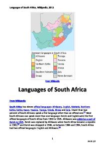
performance. Also empirically, the need to take explicit account of the so-called second nature geography aspect of a spatial data set has become evident in recent years (see Rey and Janikas (2005) and Abreu, de Groot and Florax (2005) for a good overview). Several studies have already made use of econometric techniques that take explicit account of the spatial aspect of a regional data set when looking at the evolution of income per capita. Examples are Rey and Montouri (1999), Le Gallo (2004), Le Gallo and Dall’Erba (2006), Dall’Erba (2005), Fingleton (1999), Fingleton and Lopez-Bazo (2006), Lopez-Bazo et al. (2004), Mossi et al. (2003) and Bosker (2007), all showing that a region’s location vis-à-vis other regions substantially affects a region’s own economic development. In this section we therefore take explicit account of the spatial context of our data set in the Markov chain analysis and look for evidence on the effect that economic development in a region’s neighbors has on a region itself. Before going into the details and showing the results of these space-incorporating methods, Figure 4 gives a preliminary look at the spatial aspect of the distribution of regional incomes in South Africa. The darker colored a region on the map, the higher GDP per capita compared to the national average.
By looking at the map one can immediately see patterns of concentration of economic activity, specifically in Gauteng (with Johannesburg and Pretoria as main cities) and the Western Cape (with Cape Town as main city), already suggesting some degree of spatial interdependence. To formally test for spatial autocorrelation, that is the clustering of regions with a (dis)similar realization of a random variable (here upward or downward mobility in the discretized income distribution), in the sample of South African
17
regions, we calculate the Cliff and Ord (1981) BB-statistic for both upward and downward mobility in the income distribution. It checks if, when a region moves up (down) in the discretized distribution, its neighbors are more likely to move up (down) than other regions, indicating positive spatial autocorrelation, or are less likely to do so than other regions, indicating negative spatial autocorrelation. The statistic is calculated as follows:
(6)
BB =
1 ∑∑ wij di d j 2 i j
where di = 1 if a region has moved up (down) in the discretized income distribution when testing for spatial autocorrelation in upward (downward) mobility and 0 otherwise. wij measures the ‘strength’ of the spatial interaction between regions i and j. Following most other papers using spatial econometric techniques, e.g. Fingleton and Lopez-Bazo (2006), Le Gallo (2004) and Bosker (2006; 2007), these wij are chosen to depend on the bilateral distances between the regions in the sample. This reflects the fact that transport costs and also the extent of knowledge spillovers and trade are empirically found to depend on distance (see e.g. Hummels 2001 and Audretsch and Feldman 1996). Instead of distance, other measures, such as for example trade shares or the information from input-output tables, can be argued to more accurately reflect spatial interactions between regions. These are however not readily available at the regional level, making bilateral distance an attractive alternative11. Distances are also clearly exogenous giving it an advantage from an econometric point of view over weights constructed on the basis of for example GDP or trade shares (see Anselin 1988). More formally the wij are constructed as follows:
18
(7)
Dij−1 / ∑ k Dik−1 if wij = 0
i ≠ j and Dij < Dmax else
where Dij is the distance between the centroids of two regions and the direct dependence between two regions is limited to regions closer than Dmax, the lower quartile distance of all bilateral distances between the regions in our sample (= 332 km). Dij-1 is chosen as distance decay function, a choice quite common in the empirical literature on trade and economic geography12. Finally the weights are rowstandardized, so that the spatial interaction of a region with another region depends on that other region’s relative closeness compared to the other regions in the sample. Using the thus constructed measure of spatial interaction between the regions in the sample, the BB-statistic is calculated. Table 3 below shows the BB-statistic in case of both upward and downward mobility along with the corresponding 2.5% upper and lower bound critical values, obtained by bootstrapping the empirical distribution of the statistic. When the BB-statistic is smaller (larger) than the 2.5% lower (upper) bound this means that a region is significantly less (more) likely to move up (in case of the BB-up) or down (in case of the BB-down) when its neighbor(s) make a similar move.
The results show something very interesting, the upward statistic is significant and smaller than the 2.5% lower bound indicating negative spatial autocorrelation in upward moves, i.e. if your neighbor(s) moves up in the distribution, you are less likely to make a similar move. For the downward statistic the opposite holds, if your neighbor moves down the distribution, you are significantly more likely to do so than a more distant region (significant positive spatial autocorrelation in downward
19
moves). This is quite different from earlier studies looking at e.g. Europe or the USA (see e.g. Le Gallo, 2004; Rey and Montouri, 1999 and Bosker, 2006) who find significant positive spatial autocorrelation in both upward and downward moves or no significant spatial autocorrelation at all. This finding for South Africa suggests the presence of localized growth poles, with some regions (relatively far away from each other) showing strong economic performance reflected in rising per capita income levels, leaving nearby regions behind in relative poverty. Lall and Shalizi (2003) and Ying (2000) also present significant negative spatial autocorrelation in regional growth rates in case of the Brazilian North-East and Chinese provinces respectively, which may be tentative evidence that during the development process of the national economy as a whole, regional disparities are likely to arise which corresponds to the theoretical predictions in Puga and Venables (1996). When looking at the maps in Figures 4 and 7 this finding shows itself in the high GDP per capita levels in regions surrounding for example Johannesburg, Cape Town and Durban (in Kwazulu Natal). The finding of significant spatial autocorrelation also implies that it is not correct to view the regions in the sample as isolated islands (as in the previous section) and calls for the need to use econometric techniques that take explicit note of the spatial dimension of our data. In the next two sub-sections the spatial dimension of the data set is incorporated in the Markov chain analysis in two different ways: 1.
Following the evolution of a regionally conditioned instead of the SA-wide conditioned relative income distribution (see Quah 1996b, Mossi et al. 2003, Bosker 2006, Le Gallo 2004).
2.
Estimating spatial Markov Chains (see Le Gallo 2004, Rey 2001, Mossi et al. 2003, Bosker 2006).
20
Regionally Conditioned Markov Chain Analysis Instead of looking at the evolution of regions’ GDP per capita relative to the South African level of GDP per capita, one can look at the evolution of regions’ GDP per capita relative to ‘regional GDP per capita’, i.e. a distance weighted sum of neighboring regions’ GDP per capita13. This was first suggested by Quah (1996b) and can give interesting insights in the relevance of a region’s relative location for its economic performance. More specifically the regionally conditioned income distributions can be interpreted as the part of GDP per capita that cannot be explained by location-specific factors. Figures 5 and 6 show this regionally conditioned distribution for South African regions, both as a whole and zoomed in on the left tail respectively14. Interestingly the distribution is less skewed to the left than the South African-relative GDP per capita distribution, most clearly seen by comparing the zoomed in left part of the distribution. This indicates that a substantial number of regions have income levels similar to that of their neighbors. However, note also that a small number of regions earn much more than their neighbors; the pattern in the right tail is quite similar to that of the South African-relative distribution. Merely comparing the two differently conditioned distributions does however only give suggestive evidence about whether the same regions are rich compared to their neighbors as those regions that are rich compared to the South African level of income. As in the case of Markov chain transition probabilities, this can be more formally quantified by estimating a transition matrix. Not a matrix describing the evolution over time in this case, but a matrix that tells what the probability of a region is to be rich compared to its nearby neighbors, given its income level compared to the
21
South African total (see Quah, 1996b). Table 4 below shows this matrix (where the regional distribution cut-off points are set in the same manner as in the South Africanrelative distribution).
Several interesting things can be said about these probabilities. First, only 6% of the richest South African-relative regions have income levels below 90% that of their neighbors. Second, all of the poorest South African-relative regions have income levels below 60% that of their neighbors. This corroborates the suggestive evidence provided by Figures 5 and 6 of regions with high levels of GDP per capita being scattered around the country surrounded by relatively poorer areas. Also interesting is the fact that 14% of the regions with income levels between 0.36 and 0.575 times the national GDP per capita level have income levels that are more than 1.3 times that of their neighbors giving some evidence that within the clusters of poorer regions there are also some that stand out as being ‘less poor’15. Combining this with the evidence from the calculation of the BB-statistics in the previous section, strengthens the notion of a regional economy characterized by localized regional growth poles, being those regions that are currently already enjoying a higher GDP per capita level than their (immediate) neighbors.
Figure 7 shows that such localized growth poles (the darker colored a region, the faster GDP per capita growth), can be found in e.g. Gauteng around Johannesburg and Pretoria, in the Western Cape around Cape Town and around the port cities of Durban and Richard’s Bay in KwaZulu Natal. There are also some inland regions in e.g. Limpopo province, Northwest Province and the Northern Cape that show relatively high growth rates, mainly due to the presence of natural resources.
22
The existence of such local growth poles is consistent with theoretical predictions from NEG theory (Krugman 1991; Fujita et al. 1999; Puga 1999) arguing that agglomerations, once established, continue to attract people and firms alike in search of higher wages or higher profits, eventually resulting in a strong coreperiphery pattern. Agglomerations offer workers and firms higher real wage and profit prospects respectively due to the positive externalities associated with agglomerations such as a better matching of jobs and workers, the presence of specialized inputs, knowledge spillovers and better market access (see e.g. Rosenthal and Strange 2001, Ciccone and Hall 1999 and LaFountain 2005).
Spatial Markov Chain Analysis The results in the previous sub-section provide clear evidence on the regional spread of regional economic activity in South Africa (i.e. its clustered nature). They do not provide insights into the relevance of a region’s spatial setting for the evolution of its GDP per capita level over time. The new economic geography (Puga 1999; Fujita et al. 1999) and regional science (Fingleton and Lopez-Bazo 2006; Ciccone and Hall 1999; Ciccone 2002) literature suggests however that a region’s spatial setting has a substantial impact on its subsequent economic development. A high GDP level in neighboring regions is mostly expected to have a positive effect, resulting in more trade due to increased demand for a region’s products (Krugman 1991), a higher degree of knowledge spillovers (Baldwin et al. 2001; Fingleton and Lopez-Bazo, 2006) and localized geographical externalities (Ciccone and Hall 1999). However it could also have a negative impact on the evolution of a region’s own income level as firms (Blonigen et al. 2007 provide evidence for this in case of US inward FDI in Europe) and workers (Crozet 2004 and Pons et al. 2007 provide evidence on this)
23
choose to locate in the richer (more agglomerated) neighboring region, strengthening the core-periphery pattern (Krugman 1991; Baldwin et al. 2001) in the process. In order to say something about this in case of the South African regional economy, this sub-section estimates so-called spatial Markov chains as introduced by Rey (2001). These spatial Markov chains estimate the dynamics of South Africa’sregional income distribution conditional on the distance weighted GDP per capita in neighboring regions. It gives clear insights into the influence of high/low GDP levels in a region’s neighboring regions (frequently referred to as a region’s market potential) on the evolution of GDP per capita in that region itself. To estimate these spatial Markov chains one first groups all regions according to their neighbor-relative GDP per capita16. Next, given the ordering based on neighbor-relative GDP per capita, one looks at the evolution of South African-relative GDP per capita for only those regions within a certain spatial income group. This results in five (given the five neighbor-relative income groups) 1-year transition matrices that are of dimension 5x5 (given the five South African-relative income groups); they are shown in Tables 5a-5e below.
The estimated transition probabilities show several interesting things. First, for regions with a GDP per capita level of only 60% or lower that of their neighboring regions (Tables 5a and 5b), the probability of moving up in the South African-relative income distribution is not significantly different from zero at the 10% level. On the other hand all regions that are richer than the South African-average have a lower probability of moving to a lower income group the richer they are compared to their neighboring regions (compare the last row of Table 5a-5e with each other). In general, it is mostly the case that the richer (poorer) a region compared to its neighbors, the
24
higher (lower) probability it has to move up in the South African-relative income distribution. The result of the calculation of a likelihood ratio test for spatial dependence as suggested by Bickenbach and Bode (2003), i.e. c2(23) = 70.18 with corresponding p-value: 0.00, shows that these differences are significant, strengthening the notion that a region’s transition probability significantly differs depending on its neighboring regions’ income levels (or market potential). This again confirms the earlier evidence given by the regionally conditioned distribution in Figures 5 and 6, Table 4 and the BB-statistics that the South African economy is characterized by regional growth poles. Several rich regions, scattered around the country, absorb economic activity from their neighbours, leaving them behind with relatively lower income levels. This supports the theoretical prediction made by theories stressing the advantage of agglomerations (Ciccone and Hall 1999; Rosenthal and Strange 2001 and Ciccone 2002) in the process of economic development, with the more prosperous regions attracting people and economic activity alike from the periphery establishing a strong core-periphery pattern that as predicted by new economic geography theories is not so easy to break by active government policies (see e.g. Fujita et al. 1999; Krugman 1991; Baldwin et al. 2001).
5. EXPLAINING THE OBSERVED REGIONAL INCOME DISTRIBUTION As already mentioned in section 3 the results obtained from applying (spatial) Markov Chain techniques, although giving a very clear picture of the post-Apartheid evolution of South African regional incomes, are unable to (statistically) say anything about the important factors that are driving the observed evolution. Besides looking at theory for an explanation, this section addresses this is issue by comparing some characteristics of the fastest and slowest growing regions over the period 1996 to
25
2004. These characteristics are closely linked to the factors that Nel (2002) regards as the main influences on the location of economic activity in South Africa since democratization in 1994. They also coincide with some of the determinants of South African regional income growth identified in previous empirical work (Naudé and Krugell 2003; 2006). The characteristics of the 25 fastest and 25 slowest growing regions in South Africa over the period 1996 to 2004 are shown in Table A1 and A2 in the Appendix17. This presents a diverse profile. A number of the fast growing places form part of the large metropolitan areas, that are characterised by high literacy rates and a large share of value added that is exported. Three of the other fast growers are located further away from the large hubs, but have benefited from growth of specific industries, specifically platinum mining. Then there are the smaller areas where the economies have grown fast, particularly those in the Western Cape. These places typically have smaller populations and lower population growth rates; they tend to export less, but are attractive tourist destinations. A closer look at a sectoral breakdown of gross value added (GVA) shows that these regions have particularly experienced growth in construction, retail trade, and services sectors such as postal and telecommunication services, finance and insurance, and real estate activities. The remaining fast growing places are typically quite small and have grown fast off a small base, with growth often ascribable to a single industry. Turning to the characteristics of the slowest growing regions in Table A2 shows that these regions generally have smaller populations, are less urbanised, have lower literacy rates and higher poverty rates, and little is exported from these regions. There are broadly two main groups to distinguish. First there are the regions that have been exposed to the declining fortunes of the South African gold and coal mining
26
industry. Second, there are the regions where manufacturing contracted. Specifically, this occurred in the so-called decentralised growth points that received industrial promotion subsidies under the Apartheid government and were hard hit when these were suspended in the post-Apartheid period. Overall, the profile of the fast and slow growers adds to the notion of localized growth poles, specifically in Gauteng and the Western Cape (Nel, 2002), that, by virtue of their agglomeration benefits (see Ciccone and Hall 1999; Rosenthal and Strange 2001; Fujita, et al. 1999; Puga and Venables 1996), are leaving the peripheral regions behind in (literal) poverty. The larger metropolitan areas, offering a better economic climate to both workers in terms of both income and unemployment, and to firms, in terms of human capital and export facilities, are prospering. The opening up of South Africa to the world economy seems to have exacerbated this process of increased spatial disparities even further; exporting regions are performing well in line with predictions by e.g. Hu (2002), Mansori (2003) and Gianetti (2002). These conclusions also corroborate earlier evidence provided by Naudé and Krugell (2003) who, by using more standard growth regressions, found that the faster growing regions are those with a better educated population, better market access (measured by the distance to Johannesburg) and with a greater share of exports in total output. Interestingly, the post-Apartheid regional growth process seems to largely confirm Rogerson’s (1991) prediction of a return to a spatial economy initially shaped by trade, minerals and energy, and dominated by the large metropolitan centers.
6. CONCLUSIONS The demise of Apartheid in 1994 introduced an era of opportunity for the South African economy. It marked the end of years of international sanctions, opening
27
up the economy to the rest of the world, and it provided (economic) freedom to its previously disadvantaged black population. Since the end of Apartheid the South African national economy has shown strong performance but this masks significant spatial inequality at the regional level. Using (spatial) Markov chain techniques, this paper provides clear evidence of a heavily diverging regional income distribution. Relatively poor regions are likely to remain poor or become even poorer and the richest regions will maintain or increase their lead in terms of income levels. Explicitly taking account of space furthermore shows that these richest regions are scattered around the country, acting as local growth poles absorbing economic activity from the nearby periphery. It is these few core regions that have driven recent economic growth in South Africa while ever more places on the periphery are producing less and less. The result is a strong core-periphery pattern in line with predictions from the new economic geography literature (see Fujita et al., 1999). Location, trade, education and the variable fortune of the gold mining industry seem to be important determinants of the observed evolution. When considering both the government’s past record in regional development (Nel 2002) and the predictions made by new economic geography theory (Fujita et al. 1999), this clearly sets a daunting, if not impossible challenge, for local governments in the periphery that have to fulfill their constitutional responsibility to economically develop their areas. Theory suggests that public investments in transportation, communication and education (Boarnet 1998; Démurger 2001; Mansori 2003; Lall 2007; Ravallion, 1996; Hu 2002) could provide some of the answers.
28
REFERENCES Abreu, M., H. de Groot and R. Florax. 2005. “Space and growth: a survey of empirical evidence and methods”, Région et Développement, 21, 12-43 Aghion, P. and P. Howitt. 1998. Endogenous growth theory. The MIT Press, Cambridge, Massachusetts. Anselin, L. 1988. Spatial Econometrics: Methods and Models. Kluwer, Dordrecht. Audretsch, D.B. and M.P. Feldman, 1996. “R&D spillovers and the geography of innovation and production”, American Economic Review, 86, 630-640. Aziz, J. and C.K. Duenwald, 2001. “China's provincial growth dynamics”. IMF working paper, no. 01/3. Washington. Baldwin, R., P. Martin and G. Ottaviano. 2001. “Global income divergence, trade and industrialization: the geography of growth take-offs”. Journal of Economic Growth, 6, 5-37. Bandyopadhyay, S. 2004. “Twin Peaks: Distribution Dynamics of Economic Growth across Indian States”, In: Growth, Inequality, and Poverty. Oxford University Press, Oxford, pp. 176-197. Barro, R.J. and X. Sala-I-Martin. 1991. “Convergence across states and regions”, Brookings Papers on Economic Activity, 1, 107-182. Bartholomew, D.J. 1981. Mathematical models in social science. John Wiley, Chichester, UK. Bartholomew, D.J. 1982. Stochastic models for social processes. John Wiley, Chichester, UK. Bernstein, A. & McCarthy, J. 2005. “Thinking big in small-town South Africa”, Business day, Aug. 5. Bickenbach, F. and E. Bode. 2003. “Evaluating the Markov property in studies of
29
economic convergence”, International Regional Science Review, 26, 363-392. Blonigen, B.A., R.B. Davies, G.R. Davies and H.T. Naughton. 2007. “FDI in space: spatial autoregressive in foreign direct investment”, European Economic Review, forthcoming. Boarnet, M.G. 1998. “Spillover and the locational effects of public infrastructure”, Journal of Regional Science, 38, 381-400. Bosker, E.M. 2006. “The spatial evolution of regional GDP disparities in the ‘old’ and the ‘new’ Europe”, working paper. Utrecht School of Economics, Utrecht University. Bosker, E.M., 2007. “Growth, agglomeation and convergence: a space-time analysis for European region”, Spatial Economic Analysis, 2, 91-100 Bulli, S. 2001. “Distribution dynamics and cross-country convergence: a new approach”, Scottish Journal of Political Economy, 48, 226-243. Cheshire P. and S. Magrini. 2000. “Endogenous processes in European regional growth: convergence and policy”, Growth and Change, 31, 455-479. Ciccone, A. 2002. “Agglomeration effects in Europe”, European Economic Review, 46, 213-227. Ciccone, A. and R.E. Hall. 1999. “Productivity and the density of economic activity”, American Economic Review, 86, 54-70. Cliff A.D. & J.K.Ord , 1981. Spatial processes: Models and applications. Pion, London. Crozet, M. 2004. “Do migrants follow market potential? An estimation of a new economic geography model”, Journal of Economic Geography, 4, 439-458. Dall’Erba, S. 2005. “Distribution of regional income and regional funds in Europe 1989-1999: an exploratory spatial data analysis”, The Annals of Regional
30
Science, 39. 121-148. Démurger, S. 2001. “Infrastructure development and economic growth: an explanation for regional disparities in China?”, Journal of Comparative Economics, 29, 95-117. Esteban, J.M. and D. Ray. 1994. “The measurement of polarization”, Econometrica, 62, 819-852. Fingleton, B. 1997. “Specification and testing of Markov chain models: an application to convergence in the European Union”, Oxford Bulletin of Economic and Statistics, 59, 385-403. Fingleton, B. 1999. “Estimates of time to economic convergence: an analysis of regions in the European Union”, International Regional Science Review, 22, 534. Fingleton, B. and E. Lopez-Bazo. 2003. “Explaining the distribution of manufacturing productivity in the EU regions”, In: Fingleton, B. (ed), European Regional Growth, Springer-Verlag, Berlin, pp.375-409. Fingleton, B. and E. Lopez-Bazo. 2006. “Empirical growth models with spatial effects”, Papers in Regional Science, 85, 177- 198. Friedman, M. 1992. “Do old fallacies ever die?”, Journal of Economic Literature, 30, 45-66. Fujita, M., P. Krugman and A.J. Venables, 1999. The Spatial Economy: Cities, Regions, and International Trade. MIT Press, Cambridge MA. Gianetti, M. 2002. “The effects of integration on regional disparities: convergence, divergence or both?”, European Economic Review, 46, 539-567. Hanson, G.H. 1998. “Regional adjustment to trade liberalization”, Regional Science and Urban Economics, 28, 419-444.
31
Hu, D. 2002. “Trade, rural-urban migration, and regional income disparity in developing countries: a spatial general equilibrium model inspired by the case of China”, Regional Science and Urban Economics, 32, 311-338. Hummels, D., 2001. “Toward a geography of trade costs”, working paper, Purdue University. Johnson, P.A.. 2000. A nonparametric analysis of income convergence across the US states”, Economics Letters, 69, 219-223. Krugell, W.F., Koekemoer, G. and J. Allison. 2005. “Convergence or divergence of South African cities and towns? Evidence from kernel density estimates”, Paper presented at the Biennial Conference of the Economic Society of South Africa: Development Perspectives: Is Africa Different?, Elangeni Holiday Inn, Durban, 7-9 September. Krugell, W.F. 2005. The geographical economy of South Africa. Unpublished thesis. North-West University, South Africa. Krugell, W.F. and Naudé, W.A. 2005. “The geographical economy of South Africa”, Journal of Development Perspectives, 1, 85-128. Krugman, P. 1991. “Increasing returns and economic geography”, Journal of Political Economy, 99, 483-499. Krugman, P. and R. Livas Elizondo, 1996. “Trade policy and the third world metropolis”, Journal of Development Economics, 49, 137-150. LaFountain, C. 2005. “Where do firms locate? Testing competing models of agglomeration”, Journal of Urban Economics, 58, 338-366. Lall, S.V. 2007. “Infrastructure and regional growth, growth dynamics and policy relevance for India”, The Annals of Regional Science, forthcoming. Lall, S.V. and Z. Shalizi. 2003. “Location and growth in the Brazilian northeast”,
32
Journal of Regional Science, 43, 663-681. Lee, K., H. Pesaran and R. Smith. 1998. “Growth empirics: a panel data approach – a Comment”, The Quarterly Journal of Economics, 113, 319-323. Le Gallo, J. 2004. “Space-time analysis of GDP disparities among European regions: a Markov chain approach”, International Regional Science Review, 27, 138-3. Le Gallo, J. and S. Dall’Erba. 2006. “Evaluating the temporal and spatial heterogeneity of the European convergence process, 1980-1999”, Journal of Regional Science, 46, 269-288. López-Bazo, E., E. Vayá and M. Artís. 2004. “Regional externalities and growth: evidence from European regions”, Journal of Regional Science, 44, 43-73. Magrini, S. 1999. “The evolution of income disparities among the regions of the European Union”, Regional Science and Urban Economics, 29, 257-281. Mankiw, M., D. Romer and D. Weil. 1992. “A contribution to the empirics of economic growth”, The Quarterly Journal of Economics, 107, 407-437. Mansori, K.S. 2003. “The geographic effects of trade liberalization with increasing returns in transportation”, Journal of Regional Science, 43, 249-268. Mossi, M.B., P. Aroca, I.J. Fernández and C.R. Azzoni. 2003. “Growth dynamics and space in Brazil”, International Regional Science Review, 26, 393-418. Naudé, W.A. and W.F. Krugell. 2003. “An inquiry into cities and their role in subnational economic growth in South Africa”. Journal of African Economies, 12, 476-499. Naudé, W.A. and W.F. Krugell. 2006. “Economic geography and growth in Africa: The determinants of sub-national growth in South Africa”, Papers in Regional Science, 85, 443-457. Nel, E. 2002. “South Africa’s manufacturing economy: Problems and performance”,
33
in Lemon, A. and Rogerson, C.M. (eds.), Geography and economy in South Africa and its neighbours. Aldershot: Ashgate. pp. 81-94. Pons, J., E. Paluzie, J. Silvestre and D.A. Tirado. 2007. “Testing the new economic geography: migrations and industrial agglomerations in Spain”, Journal of Regional Science, 47, 289-313. Porter, M. 2003. “The economic performance of regions”, Regional Studies, 37, 549578. Puga, D. and A.J. Venables. 1996. “The spread of industry: spatial agglomeration in economic development”, Journal of the Japanese and International Economics, 10, 440-464. Puga, D. 1999. “The rise and fall of regional inequalities”, European Economic Review, 43, 303-334. Quah, D. 1993a. “Empirical cross-section dynamics in economic growth”, European Economic Review, 37, 426-434. Quah, D. 1993b. “Galton’s fallacy and tests of the convergence hypothesis”. Scandinavian Journal of Economics, 95, 427-443. Quah, D. 1996a. “Empirics for growth and convergence”, European Economic Review, 40, 1353-1375. Quah, D. 1996b. “Regional convergence clusters across Europe”, European Economic Review, 40, 951-958. Quah, D. 1997. “Empirics for growth and distribution: polarization, stratification and convergence clubs”, Journal of Economic Growth, 2, 27-59. Ravallion, M. 1996. “Issues in measuring and modelling poverty”, Economic Journal 106, 1328-1343. Rey, S.J. 2001. “Spatial empirics for economic growth and convergence”,
34
Geographical Analysis, 33, 195-214. Rey, S.J. and M.V. Janikas. 2005. “Regional convergence, inequality and space”, Journal of Economic Geography, 5, 155-176. Rey, S.J. and B.D. Montouri. 1999. “US regional income convergence: a spatial econometric perspective”, Regional Studies, 33, 143-156. Rogerson, C.M. 1991. “Beyond racial Fordism: Restructuring industry in the “new” South Africa” Tijdschrift voor economische en sociale geografie, 82, 355-366. Rosenthal, S. and W.C. Strange. 2001. “The determinants of agglomeration”, Journal of Urban Economics, 50, 191-229. Shorrocks, A.F. 1978. “The measurement of mobility”, Econometrica, 46, 1013-1024. Silverman, B.W. 1986. Density estimation for statistics and data analysis. Chapman and Hall, London. Solow, R.M. 1956. “A contribution to the theory of economic growth”, The Quarterly Journal of Economics, 70, 65-94. Tianlun, J., J.D. Sachs and A.M. Warner. 1996. “Trends in regional inequality in China”, China Economic Review, 7, 1-21. Ying, L.G. 2000. “Measuring the spillover effects: some Chinese evidence”, Papers in Regional Science, 79, 75-89.
35
APPENDIX TABLE A1:
Fast growers, 1996-2004
Phalaborwa Volksrust Lower Umfolozi Randburg Warmbad Rustenburg George Knysna Waterberg Pretoria Wellington Sekhukhuneland Boksburg Kempton Park Tulbagh Cullinan Potgietersrus Nigel Laingsburg Sasolburg Montagu Alberton Mosselbay Vredenburg Pinetown Average (top 25)
Figure A2 Stochastic kernel South Africa vs. regionally conditioned income distribution and corresponding contour plot
TABLES
TABLE 1:
Estimated Markov 1-year transition probabilities
x SA GDP/cap < 0.17 0.17 < < 0.36 0.36 < < 0.575 0.575 < < 1.05 > 1.05 0.003* < 0.17 0.997 0 0 0 0.17 < < 0.36 0.028 0.961 0.011 0 0 0.36 < < 0.575 0 0.048 0.931 0.021 0 0.575 < < 1.05 0 0 0.048 0.936 0.016 > 1.05 0 0 0 0.026 0.974 Notes: Italic transition probabilities marked with a * are not significant at the 10% level. Each of the numbers in the table shows the probability that a region in a particular income group moves to another income group the next year. For example, a region in the lowest income group has a probability of 0.3% to move one income group up, whereas a region in the 2nd highest income group has a probability of 1.6% to make the transition to the highest income group. The p-value likelihood ratio test for time homogeneity (see Bickenbach and Bode, 2003) of the transition probabilities (splitting the sample period in half) is 0.604.
TABLE 2:
Mobility indices
Shorrock’s index 0.050
Half life 58.28
TABLE 3: BB-statistics and critical values for upward and downward mobility
UP DOWN
TABLE 4:
BB-statistic 0.033 5.872
2.5% critical value 0.095 0.006
97.5% critical value 5.738 4.673
The South Africa-relative vs. the regionally conditioned distribution
x REG GDP/cap < 0.27 0.27 < < 0.59 0.59 < < 0.9 0.9 < < 1.3 > 1.3 < 0.17 0.798 0.202 0 0 0 0.17 < < 0.36 0.172 0.491 0.287 0.050 0 0.36 < < 0.575 0 0.508 0.349 0 0.144 0.575 < < 1.05 0 0.070 0.298 0.455 0.177 > 1.05 0 0 0.061 0.234 0.706 Notes: All probabilities are significant at least at the 10% level. Each of the numbers in the table shows the probability that a region in a particular SA-relative income group is also located in a particulate regional-relative income group. For example, a region in the lowest SA-relative income group has a probability of 80% to also be in the lowest regional-relative income group, whereas a region in the 2nd lowest SA-relative income group has a probability of 20% to be in the lowest regional-relative income group.
40
TABLES 5a-5e:
Spatial Markov Chains
a. Neighbor-relative income group 1 ( GDPcap < 0.27 that of its neighbors) x SA GDP/cap < 0.17 0.17 < < 0.36 0.36 < < 0.575 0.575 < < 1.05 > 1.05 0.002* < 0.17 0.998 0 0 0 0.17 < < 0.36 0.087 0.913 0 0 0 0.36 < < 0.575 . . . . . 0.575 < < 1.05 . . . . . > 1.05 . . . . . Notes: Italic transition probabilities marked with a * are not significant at the 10% level.
b. Neighbor-relative income group 2 ( 0.27 < GDPcap < 0.59 that of its neighbors) < 0.17 0.17 < < 0.36 0.36 < < 0.575 0.575 < < 1.05 > 1.05 x SA GDP/cap 0.009* < 0.17 0.991 0 0 0 0.004* 0.17 < < 0.36 0.025 0.971 0 0 0.015* 0.36 < < 0.575 0 0.068 0.917 0 0.575 < < 1.05 0 0 0 1 0 > 1.05 . . . . . Notes: Italic transition probabilities marked with a * are not significant at the 10% level.
c. Neighbor-relative income group 3 (0.59 < GDPcap < 0.9 that of its neighbors) x SA GDP/cap < 0.17 0.17 < < 0.36 0.36 < < 0.575 0.575 < < 1.05 > 1.05 < 0.17 . . . . . 0.17 < < 0.36 0 0.981 0.019 0 0 0.36 < < 0.575 0 0.044 0.931 0.025 0 0.575 < < 1.05 0 0 0.096 0.886 0.018 > 1.05 0 0 0 0.091 0.909 Notes: Italic transition probabilities marked with a * are not significant at the 10% level.
d. Neighbor-relative income group 4 (0.9 < GDPcap < 1.3 that of its neighbors) x SA GDP/cap < 0.17 0.17 < < 0.36 0.36 < < 0.575 0.575 < < 1.05 > 1.05 < 0.17 . . . . . 0.074* 0.17 < < 0.36 0 0.926 0 0 0.36 < < 0.575 0 0.061 0.914 0.025 0 0.008* 0.575 < < 1.05 0 0 0.019 0.973 > 1.05 0 0 0 0.047 0.953 Notes: Italic transition probabilities marked with a * are not significant at the 10% level.
e. Neighbor-relative income group 5 ( GDPcap > 1.3 that of its neighbors) x SA GDP/cap < 0.17 0.17 < < 0.36 0.36 < < 0.575 0.575 < < 1.05 > 1.05 < 0.17 . . . . . 0.17 < < 0.36 . . . . . 0.013 0.36 < < 0.575 0 0 0.988 0 0.575 < < 1.05 0 0 0.059 0.901 0.040 > 1.05 0 0 0 0.013 0.987 Notes: Italic transition probabilities marked with a * are not significant at the 10% level.
41
FIGURES
1.5
FIGURE 1: South Africa’s regional income distribution 2000
2004
0
.5
1
1996
0
1 2 3 4 GDP per capita relative to SA GDP per capita
5
Notes: Over the sample period the SA GDP per capita rose from R19875 to R22125 (or in PPP adjusted 2000 I$ from I$ 7308 to I$ 9146).
1.5
FIGURE 2: South Africa’s regional income distribution – zoomed in on the left 2000
2004
0
.5
1
1996
0
.5 1 1.5 GDP per capita relative to SA GDP per capita
2
Notes: Over the sample period the SA GDP per capita rose from R19875 to R22125 (or in PPP adjusted 2000 I$ from I$ 7308 to I$ 9146).
42
FIGURE 3: Polarization between income groups 0.108
Polarization - index
0.106 0.104 0.102 0.1 0.098 0.096 0.094 1996
1997
1998
1999
2000
2001
2002
2003
2004
year
Notes: α is set to 1.5 when calculating the ER-index (see (3)). This follows Le Gallo, 2004 and Bosker, 2006 and puts a high weight on polarization.
FIGURE 4: Regional GDP per capita as a proportion of national average in 2004
Notes: Colouring goes from dark, denoting high GDP per capita, to light, denoting low GDP per capita. Namibia, Botswana, Zimbabwe, Mozambique, Swaziland and Lesotho are South Africa’s neighboring countries; the other names denote South Africa’s main provinces.
43
.8
FIGURE 5: The regionaly conditioned income distribution 2000
2004
0
.2
.4
.6
1996
0
1 2 3 4 GDP per capita relative to neighboring regions' GDP per capita
5
1
FIGURE 6: The regionaly conditioned income distribution – zoomed in on the left 2000
2004
0
.2
.4
.6
.8
1996
0
.5 1 1.5 GDP per capita relative to neighboring regions' GDP per capita
44
2
FIGURE 7: Regional GDP per capita growth between 1996 and 2004
Notes: Colouring goes from dark, denoting high GDP per capita growth, to light, denoting low GDP per capita growth. Namibia, Botswana, Zimbabwe, Mozambique, Swaziland and Lesotho are South Africa’s neighboring countries; the other names denote South Africa’s main provinces.
45
NOTES: 1
See Krugell (2005) for a detailed account of the history.
2
The distributions are obtained by kernel estimation methods using a Gaussian kernel with the optimal
bandwidth chosen using the method proposed in Silverman (1986). 3
The choice of this spatial unit of analysis comes down to the availability of data over the period 1996
to 2004. Before 2000 there were 843 municipalities in South Africa, which were then reduced to 237 to constitute so-called wall-to-wall local government. This change in demarcation complicates analysis over an extended period. At the lower level of magisterial district, data are available over the whole period. Also, the magisterial districts define the location of cities and towns, whereas the municipalities are governing bodies of larger areas. Throughout the article the terms regions or areas are used to refer to these sub-national economies. 4
The result when zooming in on the right of the distribution is not shown as this does not provide a
clearly discernable pattern over time. This is partly due to the relatively few regions with such high GDP per capita levels, making the estimated distribution more susceptible to GDP per capita changes in only a few regions. 5
We thank an anonymous referee to pointing us at the important issue of discretization.
6
All results are available upon request.
7
In Magrini (1999) for example the use of eleven income groups may approximate the continuous
distribution best but his method of boundary selection leads to having income groups, those in the tails of the distribution, containing very few observations (sometimes less than three), shedding serious doubts on the results found in and the conclusions drawn from his subsequent Markov chain analysis.
σˆ ij = mˆ ij (1 − mˆ ij ) / N i , N i = ∑ t =1 nit T −1
8
Standard errors are calculated as follows:
9
A concern may be that the degree of regional inequality provides a distorted picture of the severity of
the problem of income inequality in South Africa. It could be the case that the observed regional inequality overstates the degree of personal income inequality. This would happen when most of the poor regions are sparsely populated, so that the largest part of the population resides in the high income per capita regions. In our case, 30% of the population lived in the richest regions (with GDP per capita above the national level) in 1996 and this share declined to 27% in 2004. At the same time, 21% of the population lived in the poorest regions (with GDP per capita below 0.17 times the national level) and this share increased to 26% in 2004. (The other three income groups’ population share went from (from the lowest to highest income group) 20%, 12% and 17% in 1996 to 18%, 13% and 16% in 2004 respectively.) This clearly indicates that the high degree of regional inequality in South Africa (or its increase during the post-Apartheid period) is not due to the existence of many sparsely populated poor areas. Indeed, if anything, the evolution of regional inequality may even understate the evolution of personal income inequality, as the share of the population in the poorest regions is on the rise. 10
More specifically it denotes the number of periods it takes for the distribution to move halfway
towards its long run steady state. 11
Dall’Erba (2005) also notes the unavailability of regional input-output tables in case of European
regions and uses geographical distances instead.
46
12
Taking another value for Dmax and/or a different distance decay function (both arbitrary choices) does
not alter any of the results qualitatively. Results are available upon request. 13
The same weights as in (11) are used to construct this weighted sum of neighboring regions’ GDP
per capita. 14
The result of zooming in on the right is not shown here as this does not provide any additional
insights over Figure 5; see also footnote 4. 15
Again, estimating the corresponding stochastic kernel, shown in Figure A2 of the Appendix,
corroborates these findings. 16
Constructed in the same manner as in the previous section. As argued in Bosker (2006) conditioning
on GDP per capita relative to a region’s neighbors gives some more interesting results regarding the relevance of the economic condition(s) in a region’s immediate surroundings, than conditioning on the absolute GDP level of a region’s neighbors as done by Rey (2001). 17
A detailed description of the fast and slow growing places can be found in Krugell (2005).
service delivery in the run up to the 2006 local elections. A first step to ... development. Where railways and electric power were provided for mining, these also ...... Theory suggests that public investments in transportation, communication and ..
Retrying... Whoops! There was a problem previewing this document. Retrying... Download. Connect more apps... Try one of the apps below to open or edit this item. Skills-Development-In-Sub-Saharan-Africa-Regional-And-Sectoral-Studies.pdf. Skills-Devel
Mar 1, 2011 - World Bank Group or its Executive Directors. ... around regulations, their impact on trade and .... compliance by members with the provisions.
Aug 4, 2014 - An example of this is to be found in paragraph 94, page 61 of .... The State refused to make the State witnesses not called by the State available ...
An overview of the South African population, and the growth statistics over the last year. 2. DIGITAL PLATFORM UTILISATION. Social Media vs TV? We take ...
Jan 1, 2013 - Article Title, Victimology in South Africa (Second Edition), Robert Peacock (Ed.) : book review. Publisher: UNISA Press. Journal, New Voices in ...
Aug 4, 2014 - 39.2 The aforegoing demonstrates just how the police disturbed the scene, consequently doubt must exist as to the integrity of the scene being ...
Aug 4, 2014 - 13.4 the Accused did not blame his father for the ammunition. He simply stated the true position. Ad paragraph 19 of the heads. 14. It is not true that the Accused was a deceitful witness. There is no evidence that he ârehearsed emoti
Two sea surface temperature (SST) products, Pathfinder version 5.0 and MODIS/TERRA are evaluated .... daytime passes were processed, allowing the cloud flag (CLDICE) ... eight possible quality levels based on a hierarchical suite of tests,.
Herrenvolk Democracy and Egalitarianism in South Afri ... - Kenneth P Vickery - CSSH Vol 16 No 3 June 1974.pdf. Herrenvolk Democracy and Egalitarianism in ...
implementation scenarios of the policy are studied. Different behavioral responses in the general population are also considered. The results show that three elements are determinants for the success of such a policy: a very high testing rate, high p
Northern Ndebele live in Zimbabwe. The 1993 version of the Constitution referred to ... by approximately 61 percent of whites and 76 percent of Coloured (multiracial) people in the country. ... The fastest growing non-official language is Portuguese
active citizenship and migrants' rights, among others. The DCA SARO ... sketches and implementation plan and responsible for coordination and networking.
people in general in support of its aims and objectives and taking active ...... (a) Discipline should not be used as a means of stifling debate, or of denying.
8 don't leave home without their device. 78%. Base: Private smartphone users who use the Internet in general, Smartphone n= 1.000. Q52: To what extent do you agree to each of these statements?, Top2 Boxes; scale from 5 â completely agree to 1 â c
UNU/WIDER-UNDP, World Income Inequality Data Base, Version 1.0, 12 ..... the Gini in 1972 was also due to the entry of India which, with its gigantic population ...
South-South Cooperation for Decent Work in Africa - A Framework for Action (Draft).pdf. South-South Cooperation for Decent Work in Africa - A Framework for ...